EE364a, Winter 2007-08 Prof. S. Boyd
EE364a Homework 4 solutions
4.11 Problems involving ℓ
1
- and ℓ
∞
-norms. Formulate the following problems as LPs. Ex-
plain in detail the relation between the optimal solution of each problem and the
solution of its equivalent LP.
(a) Minimize kAx − bk
∞
(ℓ
∞
-norm approximation).
(b) Minimize kAx − bk
1
(ℓ
1
-norm approximation).
(c) Minimize kAx − bk
1
subject to kxk
∞
≤ 1.
(d) Minimize kxk
1
subject to kAx − bk
∞
≤ 1.
(e) Minimize kAx − bk
1
+ kxk
∞
.
In each problem, A ∈ R
m×n
and b ∈ R
m
are given. (See §6.1 for more problems
involving approximation and constrained approximation.)
Solution.
(a) Equivalent to the LP
minimize t
subject to Ax − b t1
Ax − b −t1.
in the variables x ∈ R
n
, t ∈ R. To see the equivalence, assume x is fixed in this
problem, and we optimize only over t. The constraints say that
−t ≤ a
T
k
x − b
k
≤ t
for each k, i.e., t ≥ |a
T
k
x − b
k
|, i.e.,
t ≥ max
k
|a
T
k
x − b
k
| = kAx − bk
∞
.
Clearly, if x is fixed, the optimal value of the LP is p
⋆
(x) = kAx −bk
∞
. Therefore
optimizing over t and x simu ltaneously is equivalent to the original problem.
(b) Equivalent to the LP
minimize 1
T
s
subject to Ax − b s
Ax − b −s
with variables x ∈ R
n
ands ∈ R
m
. Assume x is fixed in this problem, and we
optimize only over s. The constraints say that
−s
k
≤ a
T
k
x − b
k
≤ s
k
1
for each k, i.e., s
k
≥ |a
T
k
x −b
k
|. The objective function of the LP is separable, so
we achieve the optimum over s by choosing
s
k
= |a
T
k
x − b
k
|,
and obtain the optimal value p
⋆
(x) = kAx −bk
1
. Therefore optimizing over x and
s simultaneously is equivalent to the original problem.
(c) Equivalent to the LP
minimize 1
T
y
subject to −y Ax − b y
−1 x 1,
with variables x ∈ R
n
and y ∈ R
m
.
(d) Equivalent to the LP
minimize 1
T
y
subject to −y x y
−1 Ax − b 1
with variables x ∈ R
n
and y ∈ R
n
.
Another reformulation is to write x as the difference of two nonnegative vectors
x = x
+
− x
−
, and to express the problem as
minimize 1
T
x
+
+ 1
T
x
−
subject to −1 Ax
+
− Ax
−
− b 1
x
+
0, x
−
0,
with variables x
+
∈ R
n
and x
−
∈ R
n
.
(e) Equivalent to
minimize 1
T
y + t
subject to −y Ax − b y
−t1 x t1,
with variables x ∈ R
n
, y ∈ R
m
, and t ∈ R.
4.16 Minimum fuel optimal control. We consider a linear dynamical system with state
x(t) ∈ R
n
, t = 0, . . . , N, and actuator or input signal u(t) ∈ R, for t = 0, . . . , N − 1.
The dynamics of the system is given by the linear recurrence
x(t + 1) = Ax(t) + bu(t), t = 0, . . . , N − 1,
where A ∈ R
n×n
and b ∈ R
n
are given. We assume that the initial state is zero, i.e.,
x(0) = 0.
2
The minimum fuel optimal control problem is to ch oose the inputs u(0), . . . , u(N − 1)
so as to minimize the total fuel consumed, which is given by
F =
N−1
X
t=0
f(u(t)),
subject to the constraint that x(N) = x
des
, where N is the (given) time horizon, and
x
des
∈ R
n
is the (given) desired final or target state. The function f : R → R is the
fuel use map for the actuator, and gives the amount of fuel used as a function of the
actuator signal amplitude. In this problem we use
f(a) =
(
|a| |a| ≤ 1
2|a| − 1 |a| > 1.
This means that fuel use is proportional to the absolute value of the actuator signal,
for actuator signals between −1 and 1; for larger actuator signals the marginal fuel
efficiency is half.
Formulate the minimu m fuel optimal control problem as an LP.
Solution. The minimum fuel optimal control problem is equivalent to the LP
minimize 1
T
t
subject to Hu = x
des
−y u y
t y
t 2y −1,
with variables u ∈ R
N
, y ∈ R
N
, and t ∈ R, where
H =
h
A
N−1
b A
N−2
b ··· Ab b
i
.
There are several other possible LP formulations. For example, we can keep the state
trajectory x(0), . . . , x(N) as optimization variables, and replace the equality constraint
above, Hu = x
des
, with the equality constraints
x(t + 1) = Ax(t) + bu(t), t = 0, . . . , N − 1, x(0) = 0, x(N) = x
des
.
In this formulation, the variables are u ∈ R
N
, x(0), . . . , x(N) ∈ R
n
, as well as y ∈ R
N
and t ∈ R
N
.
Yet another variation is to not use the intermediate variable y introduced above, and
express the problem just in terms of the variable t ( and u):
−t u t, 2u − 1 t, −2u − 1 t,
with variables u ∈ R
N
and t ∈ R
N
.
3

4.29 Maximizing probability of satisfying a linear inequality. Let c be a random variable in
R
n
, normally distributed with mean ¯c and covariance matrix R. Consider the problem
maximize prob(c
T
x ≥ α)
subject to F x g, Ax = b.
Find the conditions under which this is equivalent to a convex or quasiconvex optimiza-
tion problem. When these conditions hold, formulate the problem as a QP, QCQP, or
SOCP (if the problem is convex), or explain how you can solve it by solving a sequence
of QP, QCQP, or SOCP feasibility problems (if the problem is quasiconvex).
Solution. Define u = c
T
x, a scalar random variable, normally distributed with mean
E u = ¯c
T
x and variance E(u − E u)
2
= x
T
Rx. The random variable
u − ¯c
T
x
√
x
T
Rx
has a normal distribution with mean zero and unit variance, so
prob(u ≥ α) = prob
u − ¯c
T
x
√
x
T
Rx
≥
α − ¯c
T
x
√
x
T
Rx
!
= 1 − Φ
α − ¯c
T
x
√
x
T
Rx
!
,
where Φ(z) =
1
√
2π
R
z
−∞
e
−t
2
/2
dt is the standard normal CDF.
To maximize prob(u ≥ α), we can minimize (α −¯c
T
x)/
√
x
T
Rx (since Φ is increasing),
i.e., solve the problem
maximize (¯c
T
x − α)/
√
x
T
Rx
subject to F x g
Ax = b.
(1)
This is not a convex optimization problem, since the objective is not concave.
The problem can, however, be solved by quasiconvex optimization provided a condtion
holds. (We’ll derive the condition below.) The objective exceeds a value t if and only
if
¯c
T
x − α ≥ t
√
x
T
Rx
holds. This last inequality is convex, in fact a second-order cone constraint, provided
t ≥ 0. So now we can state the condition: There exists a feasible x for which ¯c
T
x ≥ α.
(This condition is easily checked as an LP feasibility problem.) This condition, by the
way, can also be stated as: There exists a feasible x for which prob(u ≥ α) ≥ 1/2.
Assume that this condition holds. This means that the optimal value of our original
problem is at least 0.5, and the optimal value of the problem (1) is at least 0. This
means that we can state our problem as
maximize t
subject to F x g, Ax = b
¯c
T
x − α ≥ t
√
x
T
Rx,
4

where we can assume that t ≥ 0. This can be solved by bisection on t, by solving an
SOCP feasibility problem at each step. In other words: the function (¯c
T
x−α)/
√
x
T
Rx
is quasiconcave, provided it is nonnegative.
In fact, provided the condition above holds (i.e., there exists a feasible x with ¯c
T
x ≥ α)
we can solve the problem (1) via convex optimization. We make the change of variables
y =
x
¯c
T
x − α
, s =
1
¯c
T
x − α
,
so x = y/s. This yields the problem
minimize
q
y
T
Ry
subject to F y gs
Ay = bs
¯c
T
y − αs = 1
s ≥ 0.
4.30 A heated fluid at temperature T (degrees above ambient temperature) flows in a pipe
with fixed length and circular cross section with radius r. A layer of insulation, with
thickness w ≪ r, surrounds the pipe to reduce heat loss th rough the pipe walls. The
design variables in this problem are T , r, and w.
The heat loss is (approximately) proportional to T r/w, so over a fixed lifetime, th e
energy cost due to heat loss is given by α
1
T r/w. The cost of the pipe, which has
a fixed wall thickness, is approximately prop ortional to the total material, i.e., it is
given by α
2
r. The cost of the insulation is also approximately proportional to the total
insulation material, i.e., α
3
rw (using w ≪ r). The total cost is the sum of these three
costs.
The heat flow down the pipe is entirely due to the flow of the fluid, which has a fixed
velocity, i.e., it is given by α
4
T r
2
. The constants α
i
are all positive, as are the variables
T , r, and w.
Now the problem: maximize the total heat flow down the pipe, subject to an upper
limit C
max
on total cost, and the constraints
T
min
≤ T ≤ T
max
, r
min
≤ r ≤ r
max
, w
min
≤ w ≤ w
max
, w ≤ 0.1r.
Express this problem as a geometric program.
Solution. The problem is
maximize α
4
T r
2
subject to α
1
T w
−1
+ α
2
r + α
3
rw ≤ C
max
T
min
≤ T ≤ T
max
r
min
≤ r ≤ r
max
w
min
≤ w ≤ w
max
w ≤ 0.1r.
5
This is equivalent to the GP
minimize (1/α
4
)T
−1
r
−2
subject to (α
1
/C
max
)T w
−1
+ (α
2
/C
max
)r + (α
3
/C
max
)rw ≤ 1
(1/T
max
)T ≤ 1, T
min
T
−1
≤ 1
(1/r
max
)r ≤ 1, r
min
r
−1
≤ 1
(1/w
max
)w ≤ 1, w
min
w
−1
≤ 1
10wr
−1
≤ 1
(with variables T , r, w).
5.1 A simple example. Consider the optimization problem
minimize x
2
+ 1
subject to (x − 2)(x − 4) ≤ 0,
with variable x ∈ R.
(a) Analysis of primal problem. Give the feasible set, the optimal value, and the
optimal solution.
(b) Lagrangian and dual function. Plot the objective x
2
+ 1 versus x. On the same
plot, sh ow th e feasible set, optimal point and value, and plot the Lagrangian
L(x, λ) versus x for a few p ositive values of λ. Verify the lower bound property
(p
⋆
≥ inf
x
L(x, λ) for λ ≥ 0). Derive and sketch the Lagrange dual function g.
(c) Lagrange dual problem . State the dual problem, and verify that it is a concave
maximization problem. Find the dual optimal value and dual optimal solution
λ
⋆
. Does strong duality hold?
(d) Sensitivity analysis. Let p
⋆
(u) denote the optimal value of the problem
minimize x
2
+ 1
subject to (x − 2)(x − 4) ≤ u,
as a function of the parameter u. Plot p
⋆
(u). Verify that dp
⋆
(0)/du = −λ
⋆
.
Solution.
(a) The feasible set is the interval [2, 4]. The (unique) optimal point is x
⋆
= 2, and
the optimal value is p
⋆
= 5.
The plot shows f
0
and f
1
.
6

−1 0 1 2 3 4 5
−5
0
5
10
15
20
25
30
x
f
0
f
1
(b) The Lagrangian is
L(x, λ) = (1 + λ)x
2
− 6λx + (1 + 8λ).
The plot shows the Lagrangian L(x, λ) = f
0
+ λf
1
as a function of x for differ ent
values of λ ≥ 0. Note that the minimum value of L(x, λ) over x (i.e., g(λ)) is
always less than p
⋆
. It increases as λ varies from 0 toward 2, reaches its maximum
at λ = 2, and then decreases again as λ increases above 2. We have equality
p
⋆
= g(λ) for λ = 2.
−1 0 1 2 3 4 5
−5
0
5
10
15
20
25
30
x
@
@I
f
0
f
0
+ 1.0f
1
f
0
+ 2.0f
1
f
0
+ 3.0f
1
For λ > −1, the Lagrangian reaches its minimum at ˜x = 3λ/(1 + λ). For λ ≤ −1
it is unbounded below. Thus
g(λ) =
(
−9λ
2
/(1 + λ) + 1 + 8λ λ > −1
−∞ λ ≤ −1
which is plotted below.
7
−2 −1 0 1 2 3 4
−10
−8
−6
−4
−2
0
2
4
6
λ
g(λ)
We can verify that the dual function is concave, that its value is equal to p
⋆
= 5
for λ = 2, and less than p
⋆
for other values of λ.
(c) The Lagrange dual problem is
maximize −9λ
2
/(1 + λ) + 1 + 8λ
subject to λ ≥ 0.
The dual optimum occurs at λ = 2, with d
⋆
= 5. So for this example we can
directly observe that strong duality holds (as it must — Slater’s constraint qual-
ification is satisfied).
(d) The perturbed problem is infeasible for u < −1, since inf
x
(x
2
− 6x + 8) = −1.
For u ≥ −1, the feasible set is the inter val
[3 −
√
1 + u, 3 +
√
1 + u],
given by the two roots of x
2
− 6x + 8 = u. For −1 ≤ u ≤ 8 the optimum is
x
⋆
(u) = 3 −
√
1 + u. For u ≥ 8, the optimum is the unconstrained minimum of
f
0
, i.e., x
⋆
(u) = 0. In summary,
p
⋆
(u) =
∞ u < −1
11 + u − 6
√
1 + u −1 ≤ u ≤ 8
1 u ≥ 8.
The figure shows the optimal value function p
⋆
(u) and its epigraph.
8

−2 0 2 4 6 8 10
−2
0
2
4
6
8
10
u
p
⋆
(u)
epi p
⋆
p
⋆
(0) − λ
⋆
u
Finally, we n ote that p
⋆
(u) is a differentiable function of u, and that
dp
⋆
(0)
du
= −2 = −λ
⋆
.
9

Solutions to additional exercises
1. Minimizing a function over the probability simplex. Find simple necessary and suffi-
cient conditions for x ∈ R
n
to minimize a differentiable convex function f over the
probability simplex, {x | 1
T
x = 1, x 0}.
Solution. The simple basic optimality condition is that x is feasible, i.e., x 0,
1
T
x = 1, and that ∇f(x)
T
(y − x) ≥ 0 for all feasible y. We’ll first show this is
equivalent to
min
i=1,...,n
∇f(x)
i
≥ ∇f(x)
T
x.
To see this, suppose that ∇f(x)
T
(y − x) ≥ 0 for all feasible y. Then in particular, for
y = e
i
, we have ∇f (x)
i
≥ ∇f(x)
T
x, which is what we have above. To show the other
way, suppose that ∇f(x)
i
≥ ∇f(x)
T
x holds, for i = 1, . . . , n. Let y be feasible, i.e.,
y 0, 1
T
y = 1. Then multiplying ∇f(x)
i
≥ ∇f(x)
T
x by y
i
and summing, we get
n
X
i=1
y
i
∇f(x)
i
≥
n
X
i=1
y
i
!
∇f(x)
T
x = ∇f(x)
T
x.
The lefthand side is y
T
∇f(x), so we have ∇f(x)
T
(y − x) ≥ 0.
Now we can simplify even further. The condition above can be written as
min
i=1,...,n
∂f
∂x
i
≥
n
X
i=1
x
i
∂f
∂x
i
.
But since 1
T
x = 1, x 0, we have
min
i=1,...,n
∂f
∂x
i
≤
n
X
i=1
x
i
∂f
∂x
i
,
and it follows that
min
i=1,...,n
∂f
∂x
i
=
n
X
i=1
x
i
∂f
∂x
i
.
The right hand side is a mixture of ∂f/∂x
i
terms and equals the minimum of all of the
terms. This is possible only if x
k
= 0 whenever ∂f/∂x
k
> min
i
∂f/∂x
i
.
Thus we can write the (necessary and sufficient) optimality condition as 1
T
x = 1,
x 0, and, for each k,
x
k
> 0 ⇒
∂f
∂x
k
= min
i=1,...,n
∂f
∂x
i
.
In particular, for k’s with x
k
> 0, ∂f/∂x
k
are all equal.
2. Complex least-norm problem. We consider the complex least ℓ
p
-norm problem
minimize kxk
p
subject to Ax = b,
10
where A ∈ C
m×n
, b ∈ C
m
, and the variable is x ∈ C
n
. Here k·k
p
denotes the ℓ
p
-norm
on C
n
, defined as
kxk
p
=
n
X
i=1
|x
i
|
p
!
1/p
for p ≥ 1, and kxk
∞
= max
i=1,...,n
|x
i
|. We assume A is full rank, and m < n.
(a) Formulate the complex least ℓ
2
-norm problem as a least ℓ
2
-norm problem with
real problem data and variable. Hint. Use z = (ℜx, ℑx) ∈ R
2n
as the variable.
(b) Formulate the complex least ℓ
∞
-norm problem as an SOCP.
(c) Solve a random instance of both problems with m = 30 and n = 100. To generate
the matrix A, you can use th e Matlab command A = randn(m,n) + i*randn(m,n).
Similarly, use b = randn(m,1) + i*randn(m,1) to generate the vector b. Use
the Matlab command scatter to plot the optimal solutions of the two problems
on the complex plane, and comment (briefly) on what you observe. You can solve
the problems using th e cvx functions norm(x,2) and norm(x,inf), which are
overloaded to handle complex arguments. To utilize this feature, you will need to
declare variables to be complex in the variable statement. (In particular, you
do not have to manually form or solve the SOCP from part (b).)
Solution.
(a) Define z = (ℜx, ℑx) ∈ R
2n
, so kxk
2
2
= kzk
2
2
. The complex linear equations Ax = b
is the same as ℜ(Ax) = ℜb, ℑ(Ax) = ℑb, which in turn can be expressed as the
set of linear equations
"
ℜA −ℑA
ℑA ℜA
#
z =
"
ℜb
ℑb
#
.
Thus, the complex least ℓ
2
-norm problem can be expressed as
minimize kzk
2
subject to
"
ℜA −ℑA
ℑA ℜA
#
z =
"
ℜb
ℑb
#
.
(This is readily solved analytically).
(b) Using epigraph formulation, with new variable t, we write the problem as
minimize t
subject to
"
z
i
z
n+i
#
2
≤ t, i = 1, . . . , n
"
ℜA −ℑA
ℑA ℜA
#
z =
"
ℜb
ℑb
#
.
This is an SOCP with n second-order cone constraints (in R
3
).
11
(c) % complex minimum norm problem
%
randn(’state’,0);
m = 30; n = 100;
% generate matrix A
Are = randn(m,n); Aim = randn(m,n);
bre = randn(m,1); bim = randn(m,1);
A = Are + i*Aim;
b = bre + i*bim;
% 2-norm problem (analytical solution)
Atot = [Are -Aim; Aim Are];
btot = [bre; bim];
z_2 = Atot’*inv(Atot*Atot’)*btot;
x_2 = z_2(1:100) + i*z_2(101:200);
% 2-norm problem solution with cvx
cvx_begin
variable x(n) complex
minimize( norm(x) )
subject to
A*x == b;
cvx_end
% inf-norm problem solution with cvx
cvx_begin
variable xinf(n) complex
minimize( norm(xinf,Inf) )
subject to
A*xinf == b;
cvx_end
% scatter plot
figure(1)
scatter(real(x),imag(x)), hold on,
scatter(real(xinf),imag(xinf),[],’filled’), hold off,
axis([-0.2 0.2 -0.2 0.2]), axis square,
xlabel(’Re x’); ylabel(’Im x’);
The plot of the components of optimal p = 2 (empty circles) and p = ∞ (filled
circles) solutions is presented below. The optimal p = ∞ solution minimizes the
objective max
i=1,...,n
|x
i
| subject to Ax = b, and the scatter plot of x
i
shows that
12

almost all of them are concentrated around a circle in the complex plane. This
should be expected since we are minimizing the maximum magnitude of x
i
, and
thus almost all of x
i
’s should have about an equal magnitude |x
i
|.
−0.2 −0.15 −0.1 −0.05 0 0.05 0.1 0.15 0.2
−0.2
−0.15
−0.1
−0.05
0
0.05
0.1
0.15
0.2
ℜx
ℑx
3. Numerical perturbation analysis example. Consider the quadratic program
minimize x
2
1
+ 2x
2
2
− x
1
x
2
− x
1
subject to x
1
+ 2x
2
≤ u
1
x
1
− 4x
2
≤ u
2
,
5x
1
+ 76x
2
≤ 1,
with variables x
1
, x
2
, and parameters u
1
, u
2
.
(a) Solve this QP, for parameter values u
1
= −2, u
2
= −3, to find optimal primal
variable values x
⋆
1
and x
⋆
2
, and optimal dual variable values λ
⋆
1
, λ
⋆
2
and λ
⋆
3
. Let
p
⋆
denote the optimal objective value. Verify that the KKT conditions hold for
the optimal primal and du al variables you found (within reasonable numerical
accuracy).
Hint: See §3.6 of the CVX users’ guide to find out how to retrieve optimal du al
variables. To specify the quadratic objective, use quad_form().
(b) We will now solve some perturbed versions of the QP, with
u
1
= −2 + δ
1
, u
2
= −3 + δ
2
,
where δ
1
and δ
2
each take values from {−0.1, 0, 0.1}. (There are a total of nine
such combinations, including the original problem with δ
1
= δ
2
= 0.) For each
combination of δ
1
and δ
2
, make a prediction p
⋆
pred
of the optimal value of the
13

perturbed QP, and compare it to p
⋆
exact
, the exact optimal value of the perturbed
QP (obtained by solving the perturbed QP). Put your results in the two righthand
columns in a table with the form shown below. Check that the inequality p
⋆
pred
≤
p
⋆
exact
holds.
δ
1
δ
2
p
⋆
pred
p
⋆
exact
0 0
0 −0.1
0 0.1
−0.1 0
−0.1 −0.1
−0.1 0.1
0.1 0
0.1 −0.1
0.1 0.1
Solution.
(a) The following Matlab code sets up the simple QP and solves it using CVX:
Q = [1 -1/2; -1/2 2];
f = [-1 0]’;
A = [1 2; 1 -4; 5 76];
b = [-2 -3 1]’;
cvx_begin
variable x(2)
dual variable lambda
minimize(quad_form(x,Q)+f’*x)
subject to
lambda: A*x <= b
cvx_end
p_star = cvx_optval
When we run this, we find the optimal objective value is p
⋆
= 8.22 and the optimal
point is x
⋆
1
= −2.33, x
⋆
2
= 0.17. (This optimal point is unique since the objective
is strictly convex.) A set of optimal dual variables is λ
⋆
1
= 1.46, λ
⋆
2
= 3.77 and
λ
⋆
3
= 0.12. (The dual optimal point is unique too, but it’s harder to show this,
and it doesn’t matter anyway.)
14
The KKT conditions are
x
⋆
1
+ 2x
⋆
2
≤ u
1
, x
⋆
1
− 4x
⋆
2
≤ u
2
, 5x
⋆
1
+ 76x
⋆
2
≤ 1
λ
⋆
1
≥ 0, λ
⋆
2
≥ 0, λ
⋆
3
≥ 0
λ
⋆
1
(x
⋆
1
+ 2x
⋆
2
− u
1
) = 0, λ
⋆
2
(x
⋆
1
− 4x
⋆
2
− u
2
) = 0, λ
⋆
3
(5x
⋆
1
+ 76x
⋆
2
− 1) = 0,
2x
⋆
1
− x
⋆
2
− 1 + λ
⋆
1
+ λ
⋆
2
+ 5λ
⋆
3
= 0,
4x
⋆
2
− x
⋆
1
+ 2λ
⋆
1
− 4λ
⋆
2
+ 76λ
⋆
3
= 0.
We check these numerically. The dual variable λ
⋆
1
, λ
⋆
2
and λ
⋆
3
are all greater than
zero and the quantities
A*x-b
2*Q*x+f+A’*lambda
are found to be very small. Thus the KKT conditions are verified.
(b) The predicted optimal value is given by
p
⋆
pred
= p
⋆
− λ
⋆
1
δ
1
− λ
⋆
2
δ
2
.
The following matlab code fills in the table
arr_i = [0 -1 1];
delta = 0.1;
pa_table = [];
for i = arr_i
for j = arr_i
p_pred = p_star - [lambda(1) lambda(2)]*[i; j]*delta;
cvx_begin
variable x(2)
minimize(quad_form(x,Q)+f’*x)
subject to
A*x <= b+[i;j;0]*delta
cvx_end
p_exact = cvx_optval;
pa_table = [pa_table; i*delta j*delta p_pred p_exact]
end
end
The values obtained are
15

δ
1
δ
2
p
⋆
pred
p
⋆
exact
0 0 8.22 8.22
0 −0.1 8.60 8.70
0 0.1 7.85 7.98
−0.1 0 8.34 8.57
−0.1 −0.1 8.75 8.82
−0.1 0.1 7.99 8.32
0.1 0 8.08 8.22
0.1 −0.1 8.45 8.71
0.1 0.1 7.70 7.75
The inequality p
⋆
pred
≤ p
⋆
exact
is verified to be true in all cases.
4. FIR filter design. Consider the (symmetric, linear phase) FIR filter described by
H(ω) = a
0
+
N
X
k=1
a
k
cos kω.
The design variables are the real coefficients a = (a
0
, . . . , a
N
) ∈ R
N+1
. In this problem
we will explore the design of a low-pass filter, with specifications:
• For 0 ≤ ω ≤ π /3, 0.89 ≤ H(ω) ≤ 1.12, i.e., the filter has about ±1dB ripple in
the ‘passband’ [0, π/3].
• For ω
c
≤ ω ≤ π, |H(ω)| ≤ α. In other words, the filter achieves an attenuation
given by α in the ‘stopband’ [ω
c
, π]. ω
c
is called the ‘cutoff frequency’.
These specifications are depicted graphically in the figure below.
ω
H(ω)
0
π/3
ω
c
π
−α
0
α
0.89
1.00
1.12
16
(a) Suppose we fix ω
c
and N, and wish to maximize the stop-band attenuation, i. e.,
minimize α such that the specifications above can be met. Explain how to pose
this as a convex optimization problem.
(b) Suppose we fix N and α, and want to minimize ω
c
, i.e., we set the stopband
attenuation and filter length, and wish to minimize the ‘transition’ band (between
π/3 and ω
c
). Explain how to pose this problem as a quasiconvex optimization
problem.
(c) Now suppose we fix ω
c
and α, and wish to find the smallest N that can meet
the specifications, i.e., we seek the shortest length FIR filter that can meet the
specifications. Can this problem be posed as a convex or quasiconvex problem?
If so, explain how. If you think it cannot be, briefly and informally explain why.
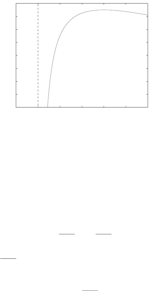
(d) Plot the optimal tradeoff curve of attenuation (α) versus cutoff frequency (ω
c
)
for N = 7. Is the set of achievable specifications convex? Briefly explain any
interesting features, e.g., flat portions, of the optimal tradeoff curve.
For this subproblem, you may sample the constraints in frequency, which means
the following. Choose K ≫ N (perhaps K ≈ 10N), and set ω
k
= kπ/K, k =
0, . . . , K. Then replace the specifications with
• For k with 0 ≤ ω
k
≤ π/3, 0.89 ≤ H(ω
k
) ≤ 1.12.
• For k with ω
c
≤ ω
k
≤ π, |H(ω
k
)| ≤ α.
With this approximation, the problem in part (a) becomes an LP, which allows
you to solve part (d) numerically.
Solution.
(a) The first problem can be expressed as
minimize α
subject to f
1
(a) ≤ 1.12
f
2
(a) ≥ 0.89
f
3
(a) ≤ α
f
4
(a) ≥ −α
(2)
where
f
1
(a) = sup
0≤ω≤π/3
H(ω), f
2
(a) = inf
0≤ω≤π/3
H(ω),
f
3
(a) = sup
ω
c
≤ω≤π
H(ω), f
4
(a) = inf
ω
c
≤ω≤π
H(ω).
Problem (2) is convex in the variables a, α because f
1
and f
3
are convex functions
(pointwise supremum of affine functions), and f
4
and f
5
are concave functions
(pointwise infimum of affine functions).
17
(b) This problem can be expressed
minimize f
5
(a)
subject to f
1
(a) ≤ 1.12
f
2
(a) ≥ 0.89
where f
1
and f
2
are the same functions as above, and
f
5
(a) = inf{Ω | − α ≤ H(ω) ≤ α for Ω ≤ ω ≤ π}.
This is a quasiconvex optimization problem in the variables a because f
1
is convex,
f
2
is concave, and f
5
is quasiconvex: its sublevel sets are
{a | f
5
(a) ≤ Ω} = {a | − α ≤ H(ω ) ≤ α for Ω ≤ ω ≤ π},
i.e., the intersection of an infinite number of halfspaces.
(c) This problem can be expressed as
minimize f
6
(a)
subject to f
1
(a) ≤ 1.12
f
2
(a) ≥ 0.89
f
3
(a) ≤ α
f
4
(a) ≥ −α
where f
1
, f
2
, f
3
, and f
4
are defined above and
f
6
(a) = min{k | a
k+1
= ··· = a
N
= 0}.
The sublevel sets of f
6
are affine sets:
{a | f
6
(a) ≤ k} = {a | a
k+1
= ··· = a
N
= 0}.
This means f
6
is a quasiconvex function, and again we have a quasiconvex opti-
mization problem.
(d) After discretizing we can express the problem in part (a) as the LP
minimize α
subject to 0.89 ≤ H(ω
i
) ≤ 1.12 for 0 ≤ ω
i
≤ π/3
−α ≤ H(ω
i
) ≤ α for ω
c
≤ ω
i
≤ π
(3)
with variables α and a. (For fixed ω
i
, H(ω
i
) is an affine function of a, hence all
constraints in this problem are linear inequalities in a and α.) We obtain the
tradeoff curve of α vs. ω
c
, by solving this LP for a sequence of values of ω
c
in the
interval (π/3, π].
Figure (1) was generated by the following matlab code.
18
clear all
N = 7;
K = 10*N;
k = [0:N]’;
w = [0:K]’/K*pi;
idx= max(find(w<=pi/3));
alphas = [];
for i=idx:length(w)
cvx_begin
variables a(N+1,1)
minimize( norm(cos(w(i:end)*k’)*a,inf) )
subject to
cos(w(1:idx)*k’)*a >= 0.89
cos(w(1:idx)*k’)*a <= 1.12
cvx_end
alphas = [alphas; cvx_optval];
end;
plot(w(idx:end),alphas,’-’);
xlabel(’wc’);
ylabel(’alpha’);
5. Minimum fuel optimal control. Solve th e minimum fuel optimal control problem de-
scribed in exercise 4.16 of Convex Optimization, for the instance with problem data
A =
−1 0.4 0.8
1 0 0
0 1 0
, b =
1
0
0.3
, x
des
=
7
2
−6
, N = 30.
You can do this by forming the LP you found in your solution of exercise 4.16, or more
directly using cvx. Plot the actuator signal u(t) as a function of time t.
Solution. The following Matlab code find s the solution
close all
clear all
n=3; % state dimension
N=30; % time horizon
A=[ -1 0.4 0.8; 1 0 0 ; 0 1 0];
b=[ 1 0 0.3]’;
19

π/3
π
0
0.2
0.4
0.6
0.8
1
α
ω
c
Figure 1 Tradeoff curve for problem 4d.
x0 = zeros(n,1);
xdes = [ 7 2 -6]’;
cvx_begin
variable X(n,N+1);
variable u(1,N);
minimize (sum(max(abs(u),2*abs(u)-1)))
subject to
X(:,2:N+1) == A*X(:,1:N)+b*u; % dynamics
X(:,1)== x0;
X(:,N+1)== xdes;
cvx_end
stairs(0:N-1,u,’linewidth’,2)
axis tight
xlabel(’t’)
ylabel(’u’)
The optimal actuator signal is shown in figure 2.
20

0 5 10 15 20 25
−0.5
0
0.5
1
1.5
2
2.5
3
u(t)
t
Figure 2 Minimum fuel actuator signal.
21
