
Oracle Rdb7
™
Introduction to SQL
Release 7.0
Part No. A40827-1
®

Introduction to SQL
Release 7.0
Part No. A40827-1
Copyright © 1993, 1996 Oracle Corporation
All rights reserved. Printed in the U.S.A.
This software was not developed for use in any nuclear, aviation, mass transit,
medical, or other inherently dangerous applications. It is the customer’s
responsibility to take all appropriate measures to ensure the safe use of such
applications if the programs are used for such purposes.
This software/documentation contains proprietary information of Oracle Corporation; it is
provided under a license agreement containing restrictions on use and disclosure and is also
protected by copyright law. Reverse engineering of the software is prohibited.
If this software/documentation is delivered to a U.S. Government Agency of the Department
of Defense, then it is delivered with Restricted Rights and the following legend is applicable:
Restricted Rights Legend
Use, duplication, or disclosure by the Government is subject to restrictions as set
forth in subparagraph (c)(1)(ii) of DFARS 252.227-7013, Rights in Technical Data and
Computer Software (October 1988).
Oracle Corporation, 500 Oracle Parkway, Redwood Shores, CA 94065.
If this software/documentation is delivered to a U.S. Government Agency not within the
Department of Defense, then it is delivered with ‘‘Restricted Rights,’’ as defined in FAR
52.227-14, Rights in Data – General, including Alternate III (June 1987).
The information in this document is subject to change without notice. If you find any
problems in the documentation, please report them to us in writing. Oracle Corporation
does not warrant that this document is error-free.
Oracle is a registered trademark of Oracle Corporation.
Oracle CDD/Repository, Rdb7, and Oracle Rdb, are trademarks of Oracle Corporation.
All other products or company names are used for identification purposes only, and may be
trademarks of their respective owners.

Contents
Send Us Your Comments ........................................... xiii
Preface ........................................................... xv
Technical Changes and New Features ............................... xix
1 Getting Started with Interactive SQL on OpenVMS
1.1 Creating a Sample Database . ................................. 1–1
1.2 Invoking Interactive SQL ..................................... 1–2
1.3 Using Online HELP ......................................... 1–3
1.4 Typing SQL Statements ...................................... 1–3
1.5 Attaching to a Database ...................................... 1–4
1.6 Detaching from a Database . . ................................. 1–4
1.7 Correcting Mistakes ......................................... 1–4
1.8 Making Interactive SQL Easier to Use . ......................... 1–5
1.8.1 Executing DCL Commands from the SQL Interactive Interface ..... 1–5
1.8.2 Defining a Logical Name for the Database ..................... 1–6
1.8.3 Using SQL Command Procedures . . ......................... 1–6
1.8.4 Controlling Session Output ................................ 1–7
1.8.5 Using Editors with SQL . . ................................. 1–7
1.8.6 Tailoring the Interactive SQL Environment .................... 1–9
2 Getting Started with Interactive SQL on Digital UNIX
2.1 Creating a Sample Database . ................................. 2–1
2.2 Invoking Interactive SQL ..................................... 2–3
2.3 Using Online HELP ......................................... 2–3
2.4 Typing SQL Statements ...................................... 2–4
2.5 Attaching to a Database ...................................... 2–4
2.6 Detaching from a Database . . ................................. 2–4
2.7 Correcting Mistakes ......................................... 2–5
iii
2.8 Making Interactive SQL Easier to Use .......................... 2–5
2.8.1 Executing Shell Commands from the SQL Interactive Interface .... 2–6
2.8.2 Defining a Configuration Parameter for the Database ............ 2–6
2.8.3 Using SQL Indirect Command Files . . . ...................... 2–6
2.8.4 Controlling Session Output . . .............................. 2–7
2.8.5 Using Editors with SQL ................................... 2–8
2.8.6 Tailoring the Interactive SQL Environment .................... 2–9
3 Displaying Information About a Database
3.1 Using the SHOW Statement .................................. 3–1
3.1.1 Adding Comments to Database Displays ...................... 3–6
3.1.2 Commonly Used Show Statements ........................... 3–9
3.2 Summarizing Database Structures in a Diagram ................... 3–10
4 Retrieving Data
4.1 Using Examples in This Chapter . .............................. 4–1
4.2 Retrieving Data from a Table or View ........................... 4–2
4.3 Using Alternative Column Names .............................. 4–5
4.4 Displaying Value Expressions and Literal Strings .................. 4–6
4.5 Displaying Concatenated Strings . .............................. 4–8
4.6 Eliminating Duplicate Rows (DISTINCT) . . ...................... 4–9
4.7 Using the ALL Keyword to Include All Rows Explicitly . ............. 4–11
4.8 Retrieving Rows in Sorted Order (ORDER BY) .................... 4–11
4.9 Retrieving a Limited Number of Rows (LIMIT TO) ................. 4–15
4.10 Retrieving a Subset of Rows (WHERE) .......................... 4–16
4.10.1 Understanding Predicates . . . .............................. 4–18
4.10.2 Using Comparison Predicates .............................. 4–18
4.10.3 Using the Range Test Predicate ([NOT] BETWEEN) ............. 4–21
4.10.4 Using the Set Membership Predicate ([NOT] IN) . . . ............. 4–23
4.10.5 Using String Comparison Predicates . . . ...................... 4–26
4.10.6 Using the Pattern Matching Predicate ([NOT] LIKE) ............ 4–27
4.10.7 Using the Null Value Predicate (IS [NOT] NULL) . . ............. 4–31
4.11 Using Conditional and Boolean Operators . . ...................... 4–35
4.11.1 Evaluating Search Conditions .............................. 4–37
4.12 Summary Queries .......................................... 4–38
4.12.1 Performing Calculations on Columns . . . ...................... 4–39
4.12.2 Computing a Total (SUM) . . . .............................. 4–39
4.12.3 Computing an Average (AVG) .............................. 4–40
4.12.4 Finding Minimum and Maximum Values (MIN and MAX) . . . ..... 4–40
4.12.5 Counting Rows (COUNT) .................................. 4–41
4.12.6 When Functions Return Empty Rows . . ...................... 4–42
iv
4.13 Built-In Functions . ......................................... 4–43
4.13.1 Converting Data Types (CAST) ............................. 4–44
4.13.2 Returning String Length (CHARACTER_LENGTH and
OCTET_LENGTH) ....................................... 4–45
4.13.3 Displaying a Substring (SUBSTRING) ........................ 4–46
4.13.4 Removing Leading or Trailing Characters (TRIM) ............... 4–47
4.13.5 Locating a Substring (POSITION) . . ......................... 4–49
4.13.6 Changing Character Case (UPPER and LOWER) ............... 4–51
4.13.7 Translating Character Strings (TRANSLATE) . . ................ 4–52
4.14 Using Column Functions on Groups of Rows (GROUP BY) . . . ........ 4–53
4.14.1 Using a Search Condition to Limit Groups (HAVING) ............ 4–56
4.15 Retrieving Data from Multiple Tables (JOINS) .................... 4–58
4.15.1 Crossing Two Tables ...................................... 4–58
4.15.2 Joining Two Tables ....................................... 4–60
4.15.3 Using Correlation Names . ................................. 4–63
4.15.4 Using Explicit Join Syntax ................................. 4–64
4.15.5 Combining a Join Condition with a Regular Condition . . . ........ 4–66
4.15.6 Joining More Than Two Tables ............................. 4–67
4.15.7 Using a Table as a Bridge Between Two Other Tables ............ 4–68
4.15.8 Joining a Table with Itself to Answer Reflexive Questions . ........ 4–70
4.16 Testing SQL Statements Before Accessing the Database ............. 4–72
5 Inserting, Updating, and Deleting Data
5.1 Transactions ............................................... 5–1
5.1.1 Starting a Transaction . . . ................................. 5–1
5.1.2 Ending a Transaction ..................................... 5–2
5.2 Inserting New Rows ......................................... 5–3
5.2.1 Default Column Values . . ................................. 5–7
5.2.2 Using the INSERT Statement to Copy Data from Another Table . . . 5–9
5.2.3 Inserting the Results of a Calculated Column Expression . ........ 5–11
5.3 Updating Rows ............................................. 5–11
5.4 Changing Data Using Views . ................................. 5–13
5.5 Conversion of Data Type in INSERT and UPDATE Statements ....... 5–15
5.6 Deleting Rows ............................................. 5–17
5.7 Using Special SQL Keywords . ................................. 5–19
5.7.1 Using the CURRENT_USER Keyword ........................ 5–19
5.7.2 Using the CURRENT_TIMESTAMP Keyword . . ................ 5–21
5.8 How Constraints Affect Write Operations ........................ 5–23
5.9 Write Operations That Activate Triggers ......................... 5–26
v
6 Advanced Data Manipulation
6.1 Using Subqueries to Answer Complex Questions ................... 6–1
6.1.1 Developing Subqueries .................................... 6–1
6.1.2 Subqueries and Joins ..................................... 6–3
6.1.3 General Format for Using Subqueries . . ...................... 6–4
6.1.4 Building a Subquery Structure ............................. 6–5
6.1.5 Using Different Values with Each Evaluation of the Outer Query . . . 6–7
6.1.6 Checking for the Existence of Rows .......................... 6–9
6.1.7 Using Several Levels of Subqueries .......................... 6–11
6.1.8 Using a Quantified Predicate to Compare Column Values with a Set
of Values .............................................. 6–14
6.1.9 Using the ORDER BY and LIMIT TO Clauses in Subqueries . ..... 6–16
6.2 UNION: Combining the Result of SELECT Statements . ............. 6–17
6.2.1 Using the UNION Clause with the ALL Qualifier . . ............. 6–19
6.2.2 Using the UNION clause Without the ALL Qualifier ............. 6–20
6.3 Using Outer Joins .......................................... 6–22
6.4 Derived Tables ............................................. 6–25
6.5 Retrieving Data from System Tables ............................ 6–26
6.6 Creating Views ............................................. 6–30
6.6.1 Simple and Complex Views . . .............................. 6–30
7 Using Multischema Databases
7.1 Multischema Sample Database . . .............................. 7–1
7.2 Multischema Database Structure . .............................. 7–2
7.3 Accessing a Multischema Database ............................. 7–3
7.4 Displaying Multischema Database Information .................... 7–4
7.4.1 Displaying Specific Schema Elements . . ...................... 7–7
7.4.2 Using the SHOW Statement with a Full Element Name .......... 7–7
7.4.3 Using the SET Statement to Access a Specific Catalog and
Schema . .............................................. 7–8
7.4.4 Setting a New Default Schema ............................. 7–10
7.5 Querying a Multischema Database with SQL ..................... 7–13
7.5.1 Joining Tables in a Multischema Database .................... 7–15
7.5.2 Using an SQL Command File to Set the Default Catalog and
Schema . .............................................. 7–17
7.6 Multischema Access Modes ................................... 7–18
7.6.1 Multischema Database Element Naming ...................... 7–19
7.6.2 Assigning Stored Names .................................. 7–20
vi
7.6.3 Matching SQL Names to Stored Names ....................... 7–22
7.6.3.1 Using the SHOW Statement to Match SQL Names to Stored
Names ............................................. 7–22
7.6.3.2 Using the System Tables to Match SQL Names to Stored
Names ............................................. 7–23
8 Using Date-Time Data Types
8.1 Date-Time Data Types and Functions . . ......................... 8–1
8.1.1 DATE VMS Data Type . . . ................................. 8–3
8.1.2 DATE ANSI Data Type . . ................................. 8–5
8.1.3 TIMESTAMP Data Type . ................................. 8–6
8.1.4 TIME Data Type ........................................ 8–7
8.1.5 INTERVAL Data Type . . . ................................. 8–8
8.1.6 Using the INTERVAL Data Type . . . ......................... 8–10
8.2 Date-Time Data Type Literal Formats . . ......................... 8–11
8.3 Using the EXTRACT Function ................................. 8–13
8.4 Rules for Performing Date-Time Arithmetic ....................... 8–15
Index
Examples
3–1 Displaying All Tables ..................................... 3–1
3–2 Displaying Information on a Particular Table . . ................ 3–2
3–3 Displaying All Views ..................................... 3–2
3–4 Displaying Information on a Particular View . . . ................ 3–3
3–5 Displaying Domain Information ............................. 3–4
3–6 Displaying Index Information .............................. 3–5
3–7 Using the COMMENT ON Statement ........................ 3–6
4–1 Selecting One or More Columns from a Table . . ................ 4–2
4–2 Selecting All Columns from a Table . ......................... 4–4
4–3 Displaying Null Values. . . ................................. 4–4
4–4 Assigning an Alternative Column Name ...................... 4–5
4–5 Displaying Computed Values and Literal Strings ............... 4–7
4–6 Using an Alternative Column Name Instead of a Literal String .... 4–7
4–7 Dividing Column Values . . ................................. 4–8
4–8 Concatenating Strings from Two Columns ..................... 4–9
4–9 Using the DISTINCT Keyword to Eliminate Duplicates . . ........ 4–10
vii
4–10 Using the ORDER BY Clause with the Default Setting ........... 4–12
4–11 Using the ORDER BY Clause with the DESC Keyword ........... 4–13
4–12 Using the ORDER BY Clause with a Computed Column .......... 4–14
4–13 Using the ORDER BY Clause with Two Sort Keys . ............. 4–15
4–14 Using the LIMIT TO Clause to Control Output ................. 4–16
4–15 Using the WHERE Clause . . . .............................. 4–17
4–16 Using Comparison Operators . .............................. 4–19
4–17 Using the BETWEEN Predicate ............................. 4–21
4–18 Using the BETWEEN Predicate with Character Data ............ 4–22
4–19 Using the NOT BETWEEN Predicate . . ...................... 4–23
4–20 Using the IN Predicate ................................... 4–24
4–21 Using the NOT IN Predicate . .............................. 4–25
4–22 Using the STARTING WITH and CONTAINING Predicates . . ..... 4–27
4–23 Using the LIKE Predicate . . . .............................. 4–28
4–24 Using the NOT LIKE Predicate ............................. 4–31
4–25 Checking for Null Values .................................. 4–32
4–26 Using the IS NULL Predicate with Another Predicate ........... 4–33
4–27 Using the IS NOT NULL Predicate .......................... 4–34
4–28 Combining Conditions in Predicates . . . ...................... 4–35
4–29 Using Parentheses to Group Predicates . ...................... 4–38
4–30 Using the SUM Function .................................. 4–40
4–31 Using the AVG Function .................................. 4–40
4–32 Using the MAX and MIN Functions .......................... 4–41
4–33 Using the COUNT Function . . .............................. 4–42
4–34 Using the CAST Function . . . .............................. 4–45
4–35 Using the CHARACTER_LENGTH Function ................... 4–46
4–36 Using the SUBSTRING Function ............................ 4–47
4–37 Using the TRIM Function . . . .............................. 4–48
4–38 Using the POSITION Function ............................. 4–50
4–39 Using the LOWER and UPPER Functions ..................... 4–52
4–40 Organizing Tables Using the GROUP BY Clause . . . ............. 4–53
4–41 Using the GROUP BY Clause with Two Columns . . ............. 4–55
4–42 Using the HAVING Clause . . . .............................. 4–57
4–43 Crossing Two Tables ...................................... 4–60
4–44 Joining Two Tables . ...................................... 4–62
4–45 Using Correlation Names .................................. 4–64
4–46 Using Explicit Join Syntax. . . .............................. 4–65
viii
4–47 Combining a Join Condition with a Regular Condition . . . ........ 4–66
4–48 Joining EMPLOYEES, DEGREES, and COLLEGES ............. 4–67
4–49 Using the DEGREES Table as a Bridge ....................... 4–70
4–50 Joining SALARY_HISTORY with Itself ....................... 4–71
4–51 Testing SQL Queries ..................................... 4–72
5–1 Inserting a New Row (Part 1 of 2) . . ......................... 5–4
5–2 Inserting a New Row (Part 2 of 2) . . ......................... 5–5
5–3 Listing Default Values for the EMPLOYEES Table .............. 5–7
5–4 Inserting an Incomplete Row ............................... 5–9
5–5 Copying a Row from One Table to Another .................... 5–10
5–6 Inserting a Calculated Value into a Row ...................... 5–11
5–7 Updating Rows . ......................................... 5–12
5–8 Displaying a Read-Only View ............................... 5–14
5–9 Inserting an Unmatched Data Type . ......................... 5–15
5–10 Deleting Rows . ......................................... 5–18
5–11 Inserting and Retrieving the CURRENT_USER Value . . . ........ 5–20
5–12 Using the CURRENT_TIMESTAMP Keyword . . ................ 5–22
5–13 Looking at Primary and Foreign Key Constraints ............... 5–25
5–14 Violation of a Primary Key Constraint ........................ 5–26
5–15 Using the SHOW TRIGGERS Statement ...................... 5–27
5–16 Values of EMPLOYEES and JOB_HISTORY Before the Update .... 5–28
6–1 Substituting a Subquery for a Constant Value . . ................ 6–2
6–2 Using a Subquery to Obtain Data from Multiple Tables . . ........ 6–6
6–3 Referring to the Outer Query ............................... 6–8
6–4 Using the EXISTS Predicate ............................... 6–9
6–5 Using the SINGLE Predicate ............................... 6–11
6–6 Nested Subqueries ....................................... 6–12
6–7 Using the ANY and ALL Keywords with Subqueries ............. 6–15
6–8 Using the ORDER BY and LIMIT TO Clauses in a Subquery ...... 6–16
6–9 Two Queries Before the UNION Operation Is Performed . . ........ 6–18
6–10 Combining Two Queries Using the UNION ALL Clause . . ........ 6–19
6–11 Combining Two Queries Using the UNION Clause .............. 6–20
6–12 Using an Outer Join ..................................... 6–24
6–13 Using a Derived Table . . . ................................. 6–26
6–14 Querying a System Table . ................................. 6–28
6–15 Defining a Simple View . . ................................. 6–31
6–16 Defining a Complex View . ................................. 6–32
ix
7–1 Displaying Catalogs and Schemas ........................... 7–4
7–2 Displaying Database Tables . . .............................. 7–6
7–3 Displaying Database Views . . .............................. 7–7
7–4 Specifying Full Element Names ............................. 7–8
7–5 Setting Access to a Specific Catalog and Schema . . . ............. 7–9
7–6 Changing the Default Schema .............................. 7–10
7–7 Displaying Elements from Other Schemas ..................... 7–11
7–8 Using the SHOW VIEWS Statement . . . ...................... 7–12
7–9 Querying Tables in the Default Catalog and Schema ............. 7–13
7–10 Querying Tables in Other Schemas .......................... 7–15
7–11 Joining Tables in the Same Schema .......................... 7–15
7–12 Joining Tables Across Schemas ............................. 7–17
7–13 Command File Content: start_multi.sql . ...................... 7–18
7–14 Displaying SQL Names for Database Elements ................. 7–19
7–15 Displaying Stored Table Names ............................. 7–20
7–16 Using the SHOW Statement to Display Stored Names ........... 7–22
7–17 Displaying System Tables . . . .............................. 7–23
7–18 Displaying the Stored Names for the Tables in the Database . ..... 7–24
7–19 Finding the Table’s SQL Name and Schema ID ................. 7–26
7–20 Finding the Schema Name and Identifying the Parent Catalog ..... 7–27
7–21 Displaying the Catalog Identifier and Name ................... 7–28
8–1 DATE VMS Specification .................................. 8–4
8–2 DATE ANSI Specification .................................. 8–5
8–3 TIMESTAMP Specification . . . .............................. 8–6
8–4 Displaying Data in TIME Format ........................... 8–8
8–5 INTERVAL Specification .................................. 8–10
8–6 Using INTERVAL with the DATE Data Type ................... 8–12
8–7 Extracting Date-Time Information ........................... 8–14
8–8 Using CURRENT_DATE and INTERVAL ..................... 8–16
8–9 Subtracting TIME . ...................................... 8–17
8–10 Using SUM with INTERVAL . .............................. 8–17
x
Figures
3–1 Conceptual Structure of the mf_personnel Database ............. 3–12
4–1 Using a Table as a Bridge Between Two Other Tables ............ 4–69
7–1 Multischema Database . . . ................................. 7–3
Tables
1–1 Common Commands for Creating Sample Databases ............ 1–2
1–2 Statements That Control Output . . . ......................... 1–7
1–3 SQL Editing Statements . ................................. 1–8
2–1 Common Commands for Creating Sample Databases ............ 2–3
2–2 Statements That Control Output . . . ......................... 2–8
3–1 Commonly Used SHOW Statements ......................... 3–10
4–1 Summary of LIKE Pattern Matching ......................... 4–30
4–2 Boolean Operators ....................................... 4–35
4–3 Aggregate Functions ..................................... 4–39
4–4 Two Formats of the COUNT Function ........................ 4–41
4–5 Built-In Functions ....................................... 4–44
4–6 Types of Joins . ......................................... 4–61
4–7 Explicit Join Syntax ...................................... 4–64
4–8 SET EXECUTE and Associated Statements . . . ................ 4–72
5–1 Ending a Transaction ..................................... 5–2
5–2 Ending a Transaction When Exiting the Interactive Session ....... 5–2
5–3 VALUES Clause Entries . ................................. 5–3
5–4 SQL Keywords . ......................................... 5–19
5–5 Constraints on Tables and Columns . ......................... 5–24
6–1 Outer Join Types ........................................ 6–22
7–1 Using the SHOW Statement to Display a List of Elements ........ 7–4
7–2 Using the SHOW Statement to Display Schema Elements ........ 7–7
8–1 Date-Time Data Types . . . ................................. 8–2
8–2 Date-Time Functions ..................................... 8–3
8–3 Interval Qualifiers ....................................... 8–8
8–4 Date-Time Data Type Literal Formats ........................ 8–11
8–5 Valid Arithmetic Operations with Date-Time Data Types . ........ 8–16
xi

Send Us Your Comments
Oracle Corporation welcomes your comments and suggestions on the quality
and usefulness of this publication. Your input is an important part of the
information used for revision.
You can send comments to us in the following ways:
• Electronic mail —
• FAX —
603-897-3334 Attn: Oracle Rdb Documentation
• Postal service
Oracle Corporation
Oracle Rdb Documentation
One Oracle Drive
Nashua, NH 03062
USA
If you like, you can use the following questionnaire to give us feedback. (Edit
the online release notes file, extract a copy of this questionnaire, and send it to
us.)
Name Title
Company Department
Mailing Address Telephone Number
Book Title Version Number
• Did you find any errors?
• Is the information clearly presented?
• Do you need more information? If so, where?
xiii
• Are the examples correct? Do you need more examples?
• What features did you like most about this manual?
If you find any errors or have any other suggestions for improvement, please
indicate the chapter, section, and page number (if available).
xiv

Preface
SQL (structured query language) serves as the primary database interface
supplied with Oracle Rdb software.
Purpose of This Manual
This manual provides an introduction to the SQL language as implemented
by Oracle Rdb and the interactive SQL interface. This manual introduces you
to SQL language through an extensive set of examples. You can enter and
experiment with the examples interactively at your terminal or workstation
using an Oracle Rdb sample database. You create the sample database from
files supplied with the kit. To become familiar with using SQL with host
language programs, read the Oracle Rdb7 Guide to SQL Programming.
Intended Audience
This manual primarily addresses users who have little or no knowledge of SQL
and who want a basic understanding of the SQL interactive interface. To profit
most from your reading, you should know the basic concepts and terminology
of relational database management systems and of your operating system.
How This Manual Is Organized
This manual contains the following chapters:
Chapter 1 Provides an overview of the SQL interactive environment on
OpenVMS.
Chapter 2 Provides an overview of the SQL interactive environment on
Digital UNIX.
Chapter 3 Describes how to display information about an Oracle Rdb
database using interactive SQL.
Chapter 4 Describes how to retrieve data from an Oracle Rdb database
using basic SQL statements.
xv
Chapter 5 Explains how to insert, update, and delete data in an Oracle
Rdb database using interactive SQL.
Chapter 6 Explains how to construct advanced queries using
interactive SQL.
Chapter 7 Provides information about naming and storing schema
objects in a multischema Oracle Rdb database.
Chapter 8 Explains how to use date-time data types in interactive
SQL.
Related Manuals
The following manuals contain information pertinent to your work with SQL:
• Oracle Rdb7 SQL Reference Manual
• Oracle Rdb7 Guide to SQL Programming
• Oracle Rdb7 Guide to Database Design and Definition
• Oracle Rdb7 Release Notes
• Oracle Rdb7 Installation and Configuration Guide
See the Oracle Rdb7 Release Notes for a complete list of the manuals in the
Oracle Rdb documentation set.
Conventions
In examples, an implied carriage return occurs at the end of each line, unless
otherwise noted. You must press the Return key at the end of a line of input.
OpenVMS means both the OpenVMS Alpha operating system and the
OpenVMS VAX operating system.
Oracle Rdb refers to Oracle Rdb for OpenVMS and Oracle Rdb for
Digital UNIX software. Version 7.0 of Oracle Rdb software is often referred to
as V7.0.
The SQL interface to Oracle Rdb is referred to as SQL. This interface is the
Oracle Rdb implementation of the SQL standard ANSI X3.135-1992, ISO
9075:1992, commonly referred to as the ANSI/ISO standard or SQL92.
Oracle CDD/Repository software is referred to as the dictionary, the data
dictionary, or the repository.
xvi

The following conventions are also used in this manual:
Ctrl/x
This symbol indicates that you hold down the Ctrl (control) key while
you press another key or mouse button (indicated here by x).
Return
In examples, a boxed symbol indicates that you must press the named
key. For example, this symbol indicates the Return key.
.
.
.
Vertical ellipsis points in an example mean that information not directly
related to the example has been omitted.
... Horizontal ellipsis points in statements or commands mean that parts
of the statement or command not directly related to the example have
been omitted.
e, f, t Index entries in the printed manual may have a lowercase e, f, or t
following the page number; the e, f, or t is a reference to the example,
figure, or table, respectively, on that page.
boldface
text
Boldface type in text indicates a term defined in the text.
< > Angle brackets enclose user-supplied names.
[ ] Brackets enclose optional clauses from which you can choose one or
none. When brackets enclose several options, the options are separated
by the word ‘‘or.’’
$ The dollar sign represents the DIGITAL Command Language prompt in
OpenVMS and the Bourne shell prompt in Digital UNIX.
Oracle Rdb for Digital UNIX Samples Directory
This manual uses the term Samples directory to refer to the
/usr/lib/dbs/sql/vnn/examples subdirectory, where nn is replaced with the
version of Oracle Rdb you are using. (For example, if you are using Oracle Rdb
V7.0, the samples directory is /usr/lib/dbs/sql/v70/examples.) This subdirectory
contains sample programs and the script that creates the sample databases.
xvii

Technical Changes and New Features
This section identifies the new and updated portions of this manual since it
was last released with Version 6.0 of Oracle Rdb.
The major new features and technical changes that are described in this
manual include:
• Examples use the mf_personnel database
Prior to this update of the Oracle Rdb7 Introduction to SQL, examples used
the single-file personnel database. Examples now use use the multifile
mf_personnel database.
• TRIM built-in function
The TRIM built-in function lets you remove leading and trailing characters
from a character string. Refer to Section 4.13.4 for a description of the
TRIM built-in function.
• POSITION built-in function
The POSITION built-in function lets you search for a particular substring
within another string. Refer to Section 4.13.5 for a description of the
POSITION built-in function.
• Multistring comments
You can now specify comments that contain more than one string literal.
This was implemented as a workaround to the limitation that comments
can only be 1,024 characters in length. See Section 3.1.1 for a description
of the COMMENT ON statement.
xix

1
Getting Started with Interactive SQL on
OpenVMS
SQL is a data definition and data manipulation language for relational
databases; it is one of the interfaces supplied with Oracle Rdb. By using SQL
you can create a database, load it with data, and read and update both data
and data definitions. Variations of SQL are offered by most major vendors for
their relational database products. This fact often makes SQL the interface of
choice at sites using relational database products from a variety of vendors.
This manual discusses data manipulation using SQL. For an extensive
discussion of data definition using SQL, see the Oracle Rdb7 Guide to Database
Design and Definition.
This chapter provides an overview of the SQL interactive environment. You
should be familiar with the basic terms and concepts of relational database
management systems generally, and with SQL specifically.
1.1 Creating a Sample Database
Throughout this manual, examples use versions of the personnel sample
database that you can build by using the files supplied with the Oracle Rdb
installation kit. You can create the database in the following three forms:
• A single-file form named personnel
• A multifile form named mf_personnel
• A multischema form named corporate_data
Most of the examples in the first part of this manual are created using the
multifile form of the personnel sample database. You can create your own
copy of the mf_personnel database in one of your directories and try the
examples for yourself. To do this, display or print the following file from the
SQL$SAMPLE directory:
about_sample_databases.txt
Getting Started with Interactive SQL on OpenVMS 1–1

This file contains instructions that explain how to create the mf_personnel
sample database.
Table 1–1 lists commands for creating the various types of sample databases
available with the Oracle Rdb kit. In this manual, the multifile mf_personnel
database without Oracle CDD/Repository is used for most of the examples. The
chapters on using multischema databases and date-time arithmetic include
examples using the multischema corporate_data sample database. You may
want to build that database in your account to practice with examples in those
chapters.
Table 1–1 Common Commands for Creating Sample Databases
Sample Database
Oracle
CDD/Repository Command
Single-file
personnel
1
No @SQL$SAMPLE:personnel
Single-file
personnel
Yes @SQL$SAMPLE:personnel SQL S CDD
Multifile
mf_personnel
No @SQL$SAMPLE:personnel SQL M NOCDD
Multifile
mf_personnel
Yes @SQL$SAMPLE:personnel SQL M CDD
Multischema
corporate_data
2
No @SQL$SAMPLE:personnel SQL S NOCDD MSDB
1
Without any parameters, the personnel.com command procedure creates a single-file personnel database without use
of Oracle CDD/Repository.
2
SQL does not allow you to store database definitions for a multischema database in Oracle CDD/Repository.
1.2 Invoking Interactive SQL
To use interactive SQL on OpenVMS, you must run the executable SQL$
image. Oracle Corporation recommends that you run this image by first
defining and then using a symbol in DIGITAL Command Language (DCL). For
repeated use, include the symbol definition in your login command file. For
example, you can define the symbol to be SQL:
$ SQL :== $SQL$
Return
1–2 Getting Started with Interactive SQL on OpenVMS

To run the SQL$ image, type the symbol and press the Return key. The SQL
prompt (SQL>) indicates that you can interactively enter SQL statements. For
example:
$ SQL
Return
SQL>
To exit interactive SQL, press Ctrl/Z or type EXIT (in full) at the SQL prompt
and press the Return key. To quit interactive SQL, causing SQL to cancel any
changes that you made to the database and to exit the SQL session, type QUIT
(in full) at the SQL prompt and press the Return key.
1.3 Using Online HELP
You can type HELP at the SQL prompt to receive assistance on using SQL
statements and understanding the concepts and components of the Oracle Rdb
system. After you type HELP followed by the Return key, a menu of topics is
displayed. The cursor will then be positioned at the Topic? prompt. Typing
any of the menu items will give you assistance on that topic. The following
example shows how to access HELP:
$ SQL
SQL> HELP
You can exit help by either pressing the Return key until you reach the prompt
from which you first entered the HELP command, or by pressing Ctrl/Z at any
point.
1.4 Typing SQL Statements
Generally, typed SQL statements have the following characteristics:
• They can continue over several lines.
• They terminate with a semicolon (;).
• You can insert comments after a double hyphen ( --).
• You can prevent the execution of an SQL statement by pressing Ctrl/Z.
The following example shows how to enter a typical SQL statement:
SQL>
SQL> -- Attach to the mf_personnel database
SQL> --
SQL> ATTACH ’FILENAME mf_personnel’;
Getting Started with Interactive SQL on OpenVMS 1–3
1.5 Attaching to a Database
Use the ATTACH statement to identify the database that you want to access.
For example, you might have created the multifile mf_personnel database in
Section 1.1. You can attach to it as follows:
$ SQL
SQL> ATTACH ’FILENAME mf_personnel’;
SQL>
Instead of using the ATTACH statement to specify the database that you want
to work with, you can have SQL automatically attach to a database after you
invoke SQL. Refer to Section 1.8.2.
1.6 Detaching from a Database
After you attach to a database in interactive SQL and complete a set of
operations, you can detach from that Oracle Rdb database in a number
of ways. The simplest way to detach from a database is by exiting your
interactive session. For example:
$ SQL
SQL> ATTACH ’FILENAME mf_personnel’;
SQL> EXIT
$
You can also detach from the current database and continue the interactive
SQL session either by entering another ATTACH statement to override the
first attach, or by entering the DISCONNECT statement as follows:
SQL> DISCONNECT DEFAULT;
SQL>
1.7 Correcting Mistakes
If you make a typing or syntax error while entering a statement, SQL displays
a message giving you information about the error and what was expected. For
example, you might make a typing error trying to attach to the mf_personnel
database:
SQL> ATTACH ’FILENAME mf_personne’;
%SQL-F-ERRATTDEC, Error attaching to database mf_personne
-RDB-E-BAD_DB_FORMAT, mf_personne does not reference a database known to Rdb
-RMS-E-FNF, file not found
-COSI-E-FNF, file not found
SQL>
1–4 Getting Started with Interactive SQL on OpenVMS

If you entered a single-line statement as shown in the preceding example, you
can press the up arrow key ( ) to display and correct the statement. But if you
made a mistake in a command that used several lines, use the EDIT statement
to correct your mistakes. When you type the EDIT keyword and press the
Return key, SQL places the last statement you entered in an editing buffer. (If
you type a digit after the EDIT keyword, SQL puts that number of preceding
statements in the buffer.)
You can correct and add to statements in the buffer by using your default text
editor. (For information about how to invoke the editor of your choice, see
Section 1.8.5.) When you exit the editor, SQL processes the statements in the
buffer. The following example shows how to invoke the EDIT statement:
SQL> EDIT
Return
.
.
.
(Correct the statements and exit the editor.
SQL displays and processes the statements.)
.
.
.
*EXIT
Return
1.8 Making Interactive SQL Easier to Use
This section describes how to make working with interactive SQL easier.
1.8.1 Executing DCL Commands from the SQL Interactive Interface
You can issue DCL (DIGITAL Command Language) commands while at the
SQL prompt within interactive SQL. Precede the command with the dollar
sign ( $ ), which informs SQL that you want to access the DCL environment.
SQL spawns a subprocess and passes the command to the operating system for
processing. For example, to display a listing of the files in the directory from
which you invoked SQL, enter the following command:
SQL> $ DIR
Directory DISK:[USER]
FILE1.TXT FILE2.COM FILE 3.PS
Total of 3 files.
SQL>
Getting Started with Interactive SQL on OpenVMS 1–5
1.8.2 Defining a Logical Name for the Database
You can more easily complete the interactive examples throughout this book
if you define the logical name SQL$DATABASE to identify the database with
which you want to work. Defining SQL$DATABASE means that you will
not have to enter the ATTACH statement to specify a database after you
invoke interactive SQL. When you enter the first SQL statement that requires
database access, SQL evaluates the logical name SQL$DATABASE to find if a
database has been assigned to it. It then accesses the database to process your
statement.
Assign only the file name to SQL$DATABASE if your system directory default
will always be the directory in which the file is located when you invoke SQL.
For example:
$ DEFINE SQL$DATABASE mf_personnel
Include the disk and directory in your file name assignment if your OpenVMS
disk and directory defaults might vary when you invoke SQL. For example:
$ DEFINE SQL$DATABASE DISK01:[FIELDMAN.DBS]mf_personnel
1.8.3 Using SQL Command Procedures
You can create an OpenVMS Record Management Services (RMS) file that
contains SQL statements, and then execute this command procedure using
interactive SQL. Command procedures are useful for storing SQL statements
that you frequently enter and for testing SQL statements that you plan to
include in programs. SQL ignores text on a line following double hyphens ( -- )
so that you can include comments in your command procedure.
A command procedure named start.sql that attaches to the mf_personnel
database and displays the database name is shown in the following example:
-- Attach to the mf_personnel database
--
ATTACH ’FILENAME mf_personnel’;
--
-- Display database name
--
SHOW DATABASE
In interactive SQL, you execute an SQL command procedure by typing the at
sign ( @ ) and then the name of the procedure. If you omit the file type, SQL
searches for the command procedure with the .sql file type. To execute the
start.sql command procedure type @start as shown in the following example:
1–6 Getting Started with Interactive SQL on OpenVMS

SQL> @start
Default alias:
Oracle Rdb database in file mf_personnel
SQL>
If you type SET VERIFY before executing the command procedure, SQL
displays the contents of the command procedure as it executes the statements.
Reference Reading
In the chapter on SQL statements in the Oracle Rdb7 SQL Reference
Manual, the sections on Execute ( @ ) and SET have more information
about SQL command procedures. In the section on the SET statement,
see the SET VERIFY information.
1.8.4 Controlling Session Output
You can use the statements in Table 1–2 to control the output from an
interactive SQL session.
Table 1–2 Statements That Control Output
If You Want to . . . Use the Statement . . .
Display a message to the user PRINT ’message-string’;
Echo commands and comments from
a command file to the screen
SET VERIFY
Stop echo SET NOVERIFY
Log the session output to a file SET OUTPUT filename
Stop the log SET NOOUTPUT
Specify the length of the output line
in the log file
SET LINE LENGTH n
1.8.5 Using Editors with SQL
Interactive SQL includes an EDIT statement that allows you to correct
mistakes that you make when entering SQL statements. The EDIT statement
invokes the text editor of your choice.
Within SQL, you can use EDT, the DEC Text Processing Utility (DECTPU), or
the DEC Language-Sensitive Editor (DEC LSE). EDT is the default text editor;
however, you can assign a logical name to invoke the editor of your choice.
Getting Started with Interactive SQL on OpenVMS 1–7

If you prefer to use DECTPU, make the following assignment:
$ ASSIGN TPU SQL$EDIT
If you prefer to use DEC LSE, make the following assignment:
$ ASSIGN LSE SQL$EDIT
Reference Reading
The chapter on SQL statements in the Oracle Rdb7 SQL Reference
Manual contains sections for the EDIT and SET statements. Read
those sections for a complete discussion of your editing options and
restrictions. In the section on the SET statement, see the SET EDIT
information.
The DEC Language-Sensitive Editor (DEC LSE) is an advanced text editor
that is layered on DECTPU.
To use DEC LSE within interactive SQL, you must first assign DEC LSE as
your default SQL editor (as described earlier in this section). In addition, you
must define the logical name LSE$ENVIRONMENT as shown below:
$ DEFINE LSE$ENVIRONMENT SYS$COMMON:[SYSLIB]LSE$SYSTEM_ENVIRONMENT.ENV
Table 1–3 lists editing statements that you can use from within SQL.
Table 1–3 SQL Editing Statements
If You Want to . . . Use the Statement . . .
Edit the last line
Edit the last statement EDIT
Edit the last n number of
statements
EDIT n
Edit all statements in the edit
buffer
EDIT *
Keep the last n statements in the
buffer
SET EDIT KEEP n
Prevent statements from accumulat-
ing in the buffer
SET EDIT NOKEEP
Clear the edit buffer SET EDIT PURGE
1–8 Getting Started with Interactive SQL on OpenVMS

You can also invoke DEC LSE from the DCL level. For example, you can type
the following command to edit a file named sample.sql:
$ LSEDIT sample.sql
Reference Reading
For more information about DEC LSE, see the DEC Language-
Sensitive Editor documentation.
1.8.6 Tailoring the Interactive SQL Environment
You can create an SQL command procedure to tailor your interactive
SQL environment. If you assign the logical name SQLINI to the full file
specification for the command procedure that you create, SQL executes
the command procedure each time you invoke SQL. This is called an SQL
initialization file. For example:
$ ASSIGN DISK01:[CHESHIRE]sqlini.sql SQLINI
Include this assignment in your login.com file if you want SQLINI defined the
same way each time you log on to your system.
Consider the following SQL command procedure, sqlini.sql:
-- sqlini.sql
--
-- Greeting
--
PRINT ’Good Morning!’;
--
-- Write the session output to a log file named sql_session.log
--
SET OUTPUT sql_session.log
--
-- Attach to the mf_personnel database
--
ATTACH ’FILENAME mf_personnel’;
--
-- Display database tables
--
SHOW TABLE
In addition to defining the logical name SQLINI in your login.com file, you
should include an assignment to SQL$EDIT if your preferred editor is not
EDT.
Getting Started with Interactive SQL on OpenVMS 1–9

2
Getting Started with Interactive SQL on
Digital UNIX
SQL is a data definition and data manipulation language for relational
databases; it is one of the interfaces supplied with Oracle Rdb. By using SQL
you can create a database, load it with data, and read and update both data
and data definitions. Variations of SQL are offered by most major vendors for
their relational database products. This fact often makes SQL the interface of
choice at sites using relational database products from a variety of vendors.
This manual discusses data manipulation using SQL. For an extensive
discussion of data definition using SQL, see the Oracle Rdb7 Guide to Database
Design and Definition.
This chapter provides an overview of the SQL interactive environment. You
should be familiar with the basic terms and concepts of relational database
management systems generally, and with SQL specifically.
2.1 Creating a Sample Database
Throughout this manual, examples use versions of the personnel sample
database that you can build by using the files supplied with the Oracle Rdb
installation kit. You can create the database in the following three forms:
• A single-file form named personnel
• A multifile form named mf_personnel
• A multischema form named corporate_data
Most of the examples in the first part of this manual are created using the
multifile form of the mf_personnel sample database. You can create your
own copy of the mf_personnel database in one of your directories and try
the examples for yourself. To do this, display or print the following file from
the Samples directory. (See the Samples Directory section in the Preface for
information on the samples directory.)
about_sample_databases.txt
Getting Started with Interactive SQL on Digital UNIX 2–1
This file contains instructions that explain how to create the mf_personnel
sample database.
Table 2–1 lists commands for creating the various types of sample databases
available with the Oracle Rdb kit.
The following shows the format of the command you enter to create a sample
database:
$ /usr/lib/dbs/sql/vnn/examples/personnel <database-form> <dir>
The directory specification and the two parameters are specified as follows:
1. vnn
Replace the subdirectory specification, vnn, with the version of Oracle Rdb
you are using. For example, if you are using Oracle Rdb V7.0, the directory
specification is as follows:
/usr/lib/dbs/sql/v70/examples/personnel
2. database-form: Enter S, M, or MSDB.
This specifies the creation of a single-file (S) database, a multifile (M)
database, or a multischema (MSDB) database. A single-file database is the
default.
You can use uppercase or lowercase to specify this parameter.
3. dir: Enter a directory specification where you want the database created.
If you do not specify this parameter, the script will prompt you for a
directory specification. If you do not provide a directory specification at
the prompt, Oracle Rdb will create the database in your present working
directory. You must terminate the directory specification with a slash ( / ).
For example, to build the multifile version and specify the directory
specification on the command line, enter the following command:
$ /usr/lib/dbs/sql/v70/examples/personnel m /tmp/
The chapters on using multischema databases and date-time arithmetic
include examples using the multischema corporate_data sample database. You
may want to build that database in your account to practice with examples in
those chapters.
2–2 Getting Started with Interactive SQL on Digital UNIX

Table 2–1 Common Commands for Creating Sample Databases
Sample Database Command
Single-file
personnel
/usr/lib/dbs/sql/v70/examples/personnel s
Multifile
mf_personnel
/usr/lib/dbs/sql/v70/examples/personnel m
Multischema
corporate_data
/usr/lib/dbs/sql/v70/examples/personnel msdb
2.2 Invoking Interactive SQL
To use interactive SQL on Digital UNIX, type sql and press the Return key:
$ sql
Return
SQL>
The SQL prompt (SQL>) indicates that you can interactively enter SQL
statements.
To exit interactive SQL, type EXIT (in full) at the SQL prompt and press the
Return key. To quit interactive SQL, causing SQL to cancel any changes that
you made to the database and to exit the SQL session, type QUIT (in full) at
the SQL prompt and press the Return key.
2.3 Using Online HELP
You can type HELP at the SQL prompt to receive assistance on using SQL
statements and understanding the concepts and components of the Oracle Rdb
system. After you type HELP followed by the Return key, a menu of topics is
displayed. The cursor will then be positioned at the "Topic?" prompt. Typing
any of the menu items will give you assistance on that topic. The following
example shows how to access HELP:
$ sql
SQL> HELP
You can exit help by either pressing the Return key until you reach the prompt
from which you first entered the HELP command, or by pressing Ctrl/d at any
point.
Getting Started with Interactive SQL on Digital UNIX 2–3
2.4 Typing SQL Statements
Generally, typed SQL statements have the following characteristics:
• They can continue over several lines.
• They terminate with a semicolon (;).
• You can insert comments after a double hyphen ( --).
The following example shows how to enter a typical SQL statement:
SQL>
SQL> -- Attach to the mf_personnel database
SQL> --
SQL> ATTACH ’FILENAME mf_personnel’;
2.5 Attaching to a Database
Use the ATTACH statement to identify the database that you want to access.
For example, you might have created the multifile mf_personnel database in
Section 2.1. You can attach to it as follows:
$ SQL
SQL> ATTACH ’FILENAME mf_personnel’;
SQL>
Instead of using the ATTACH statement to specify the database that you want
to work with, you can have SQL automatically attach to a database after you
invoke SQL. Refer to Section 2.8.2.
2.6 Detaching from a Database
After you attach to a database in interactive SQL and complete a set of
operations, you can detach from that Oracle Rdb database in a number
of ways. The simplest way to detach from a database is by exiting your
interactive session. For example:
$ SQL
SQL> ATTACH ’FILENAME mf_personnel’;
SQL> EXIT
$
You can also detach from the current database and continue the interactive
SQL session either by entering another ATTACH statement to override the
first attach, or by entering the DISCONNECT statement as follows:
SQL> DISCONNECT DEFAULT;
SQL>
2–4 Getting Started with Interactive SQL on Digital UNIX

2.7 Correcting Mistakes
If you make a typing or syntax error while entering a statement, SQL displays
a message giving you information about the error and what was expected. For
example, you might make a typing error trying to attach to the mf_personnel
database:
SQL> ATTACH ’FILENAME mf_personne’;
%SQL-F-ERRATTDEC, Error attaching to database mf_personne
-RDB-E-BAD_DB_FORMAT, /usr/db/mf_personne does not reference a database
known to Rdb
-COSI-E-FNF, file not found
SQL>
If you entered a single-line statement as shown in the example, you can press
the up arrow key ( ) to display and correct the statement. But if you made
a mistake in a command that used several lines, use the EDIT statement
to correct your mistakes. When you type the EDIT keyword and press the
Return key, SQL places the last statement you entered in an editing buffer. (If
you type a digit after the EDIT keyword, SQL puts that number of preceding
statements in the buffer.)
You can correct and add to statements in the buffer by using your default text
editor. (For information about how to invoke the editor of your choice, see
Section 2.8.5.) When you exit the editor, SQL processes the statements in the
buffer. The following example shows how to invoke the EDIT statement:
SQL> EDIT
Return
.
.
.
(Correct the statements and exit the editor.
SQL displays and processes the statements.)
.
.
.
*EXIT
Return
2.8 Making Interactive SQL Easier to Use
This section describes how to make working with interactive SQL easier.
Getting Started with Interactive SQL on Digital UNIX 2–5
2.8.1 Executing Shell Commands from the SQL Interactive Interface
You can issue shell commands while at the SQL> prompt within interactive
SQL. Simply precede the command with the dollar sign ($), which informs
SQL that you want access to the shell environment (whichever shell you were
using when you invoked interactive SQL). SQL forks a subprocess and passes
the command to the shell for processing. For example, to display a listing
of the files in the directory from which you invoked SQL, enter the following
command:
SQL> $ls
file1 file2 file3 file4
file5 file6 file7
2.8.2 Defining a Configuration Parameter for the Database
You can more easily complete the interactive examples throughout this book
if you define the configuration parameter SQL_DATABASE to identify the
database with which you want to work. Defining SQL_DATABASE means
that you will not have to enter the ATTACH statement to specify a database
after you invoke interactive SQL. When you enter the first SQL statement
that requires database access, SQL evaluates the configuration parameter
SQL_DATABASE to find if a database has been assigned to it. It then accesses
the database to process your statement.
You define SQL_DATABASE as a configuration parameter in your .dbsrc file.
Assign only the file name to SQL_DATABASE if your Digital UNIX directory
default will always be the directory in which the file is located when you invoke
SQL. For example:
$ SQL_DATABASE mf_personnel
Include the directory in your file name assignment if your Digital UNIX
directory defaults might vary when you invoke SQL. For example:
$ SQL_DATABASE /usr/fieldman/dbs/mf_personnel
2.8.3 Using SQL Indirect Command Files
You can create a flat file that contains SQL statements, and then execute
this indirect command file using interactive SQL. Indirect command files are
useful for storing SQL statements that you frequently enter and for testing
SQL statements that you plan to include in programs. SQL ignores text on a
line following double hyphens (-- ) so that you can include comments in your
command file.
2–6 Getting Started with Interactive SQL on Digital UNIX

An indirect command file named start that attaches to the mf_personnel
database and displays the database name is shown in the following example:
-- Attach to the mf_personnel database
--
ATTACH ’FILENAME mf_personnel’;
--
-- Display database name
--
SHOW DATABASE
In interactive SQL, you execute an SQL indirect command file by typing the at
sign (@ ) and then the name of the file. To execute the start indirect command
procedure type @start as shown in the following example:
SQL> @start
Default alias:
Oracle Rdb database in file mf_personnel
SQL>
If you type SET VERIFY before executing the command procedure, SQL
displays the contents of the command procedure as it executes the statements.
Reference Reading
In the chapter on SQL statements in the Oracle Rdb7 SQL Reference
Manual, the sections on Execute ( @ ) and SET have more information
about SQL command procedures. In the section on the SET statement,
see the SET VERIFY information.
2.8.4 Controlling Session Output
You can use the statements in Table 2–2 to control the output from an
interactive SQL session.
Getting Started with Interactive SQL on Digital UNIX 2–7

Table 2–2 Statements That Control Output
If You Want to . . . Use the Statement . . .
Display a message to the user PRINT ’message-string’;
Echo commands and comments from
a command file to the screen
SET VERIFY
Stop echo SET NOVERIFY
Log the session output to a file SET OUTPUT filename
Stop the log SET NOOUTPUT
Specify the length of the output line
in the log file
SET LINE LENGTH n
2.8.5 Using Editors with SQL
Interactive SQL includes an EDIT statement that allows you to correct
mistakes that you make when entering SQL statements. The EDIT statement
invokes the text editor of your choice.
The vi (visual editor) is the default text editor. However, you can assign the
configuration parameter, SQL_EDIT, or the environment variable, EDITOR, to
invoke the editor of your choice.
For example, if you prefer to use the Emacs editor, define the SQL_EDIT
configuration parameter in your .dbsrc file, as follows:
SQL_EDIT emacs
Reference Reading
The chapter on SQL statements in the Oracle Rdb7 SQL Reference
Manual contains sections for the EDIT and SET statements. Read
those sections for a complete discussion of your editing options and
restrictions. In the section on the SET statement, see the SET EDIT
information.
2–8 Getting Started with Interactive SQL on Digital UNIX
2.8.6 Tailoring the Interactive SQL Environment
You can create an SQL command file, sqlini.sql, called an SQL initialization
file, to tailor your interactive SQL. To ensure that SQL executes the
initialization file each time you invoke SQL, do one of the following:
• Ensure that your sqlini.sql file is in the same directory from which you
invoke SQL.
• Define the DBSINIT variable to point to your sqlini.sql file.
For example:
setenv DBSINIT "-i /usr/mydir/sqlini.sql"
Consider the following SQL initialization file, sqlini.sql:
-- sqlini.sql
--
-- Greeting
--
PRINT ’Good Morning!’;
--
-- Write the session output to a log file named sql_session
--
SET OUTPUT sql_session
--
-- Attach to the mf_personnel database
--
ATTACH ’FILENAME mf_personnel’;
--
-- Display database tables
--
SHOW TABLE
Getting Started with Interactive SQL on Digital UNIX 2–9

3
Displaying Information About a Database
The main method for displaying information about a database in the SQL
language is the SHOW statement. This chapter explains how to use this
statement to display information about objects stored in an Oracle Rdb
database.
3.1 Using the SHOW Statement
To display a simple list of all tables and views in a database, use the SHOW
TABLES statement, as shown in Example 3–1.
Example 3–1 Displaying All Tables
SQL> --
SQL> -- Display all tables and views:
SQL> --
SQL> SHOW TABLES
User tables in database with filename mf_personnel
CANDIDATES
COLLEGES
CURRENT_INFO A view.
CURRENT_JOB A view.
CURRENT_SALARY A view.
DEGREES
DEPARTMENTS
EMPLOYEES
JOBS
JOB_HISTORY
RESUMES
SALARY_HISTORY
WORK_STATUS
To display information about a particular table, such as the WORK_STATUS
table from the mf_personnel database, enter the SHOW TABLE statement and
specify a table name, as shown in Example 3–2.
Displaying Information About a Database 3–1
Example 3–2 Displaying Information on a Particular Table
SQL> --
SQL> -- Display information about the WORK_STATUS table:
SQL> --
SQL> SHOW TABLE WORK_STATUS
Information for table WORK_STATUS
Comment on table WORK_STATUS:
information related to work status codes
Columns for table WORK_STATUS:
Column Name Data Type Domain
----------- --------- ------
STATUS_CODE CHAR(1) STATUS_CODE_DOM
Primary Key constraint WORK_STATUS_PRIMARY_STATUS_CODE
STATUS_NAME CHAR(8) STATUS_NAME_DOM
STATUS_TYPE CHAR(14) STATUS_DESC_DOM
Table constraints for WORK_STATUS:
STATUS_NAME_VALUES
Check constraint
Table constraint for WORK_STATUS
Evaluated on COMMIT
Source:
CHECK (
STATUS_NAME IN (’ACTIVE’, ’INACTIVE’)
OR STATUS_NAME IS NULL
)
.
.
.
To display all views in the database, use the SHOW VIEWS statement, as
shown in Example 3–3.
Example 3–3 Displaying All Views
SQL> --
SQL> -- Display all views:
SQL> --
SQL> SHOW VIEWS
User tables in database with filename mf_personnel
CURRENT_INFO A view.
CURRENT_JOB A view.
CURRENT_SALARY A view.
3–2 Displaying Information About a Database

To display information about a particular view, such as the CURRENT_
SALARY view from the mf_personnel database, enter the SHOW VIEW
statement and specify a view name, as shown in Example 3–4.
Example 3–4 Displaying Information on a Particular View
SQL> --
SQL> -- Display information about the CURRENT_SALARY view:
SQL> --
SQL> SHOW VIEW CURRENT_SALARY
Information for table CURRENT_SALARY
Columns for view CURRENT_SALARY:
Column Name Data Type Domain
----------- --------- ------
LAST_NAME CHAR(14)
FIRST_NAME CHAR(10)
EMPLOYEE_ID CHAR(5)
SALARY_START DATE VMS
SALARY_AMOUNT INTEGER(2)
Source:
SELECT E.LAST_NAME,
E.FIRST_NAME,
E.EMPLOYEE_ID,
SH.SALARY_START,
SH.SALARY_AMOUNT
FROM SALARY_HISTORY SH,
EMPLOYEES E
WHERE SH.EMPLOYEE_ID = E.EMPLOYEE_ID
AND SH.SALARY_END IS NULL;
The following callouts are keyed to Example 3–4:
The view definition gives the list of columns used in the view.
This section gives the actual SQL query that is used to create the view. A
view is like a predefined query that runs when you access the view.
To list domains in the database, use the SHOW DOMAINS statement, as
shown in Example 3–5.
Displaying Information About a Database 3–3

Example 3–5 Displaying Domain Information
SQL> --
SQL> -- Display all domains:
SQL> --
SQL> SHOW DOMAINS
User domains in database with filename mf_personnel
ADDRESS_DATA_1_DOM CHAR(25)
ADDRESS_DATA_2_DOM CHAR(20)
BUDGET_DOM INTEGER
.
.
.
DATE_DOM DATE VMS
.
.
.
STATUS_NAME_DOM CHAR(8)
WAGE_CLASS_DOM CHAR(1)
YEAR_DOM SMALLINT
SQL> --
SQL> -- Display information about the DATE_DOM domain:
SQL> --
SQL> SHOW DOMAIN DATE_DOM
DATE_DOM DATE VMS
Comment: standard definition for complete dates
Edit String: DD-MMM-YYYY
The following callouts are keyed to Example 3–5:
When listing all domains, you get only the domain name and data type.
The description of a single domain includes an explanation (comment)
and the output format (edit string) for interactive SQL. DATE_DOM is a
domain that includes values of the data type DATE VMS.
DATE VMS is the default date data type on both Oracle Rdb for OpenVMS
and Oracle Rdb for Digital UNIX and corresponds to the standard
OpenVMS date. Domains can be created for other date data types that can
be used in date-time arithmetic (discussed in Chapter 8).
Edit string determines the output format for the date information.
To display information about indexes defined on a database, use the SHOW
INDEXES statement, as shown in Example 3–6.
3–4 Displaying Information About a Database

Example 3–6 Displaying Index Information
SQL> --
SQL> -- Display information about all indexes:
SQL> --
SQL> SHOW INDEXES *
User indexes in database with filename mf_personnel
Indexes on table COLLEGES:
COLL_COLLEGE_CODE with column COLLEGE_CODE
No Duplicates allowed
Type is Sorted
Compression is DISABLED
Indexes on table DEGREES:
DEG_COLLEGE_CODE with column COLLEGE_CODE
Duplicates are allowed
Type is Sorted
Compression is DISABLED
DEG_EMP_ID with column EMPLOYEE_ID
Duplicates are allowed
Type is Sorted
Compression is DISABLED
.
.
.
SQL> --
SQL> -- Display information about the indexes on the
SQL> -- SALARY_HISTORY table:
SQL> --
SQL> SHOW INDEXES ON SALARY_HISTORY
Indexes on table SALARY_HISTORY:
SH_EMPLOYEE_ID with column EMPLOYEE_ID
Duplicates are allowed
Type is Sorted
Compression is DISABLED
SQL> --
SQL> -- Display information about the DEG_EMP_ID index:
SQL> --
SQL> SHOW INDEX DEG_EMP_ID
Indexes on table DEGREES:
DEG_EMP_ID with column EMPLOYEE_ID
Duplicates are allowed
Type is Sorted
Compression is DISABLED
The following callouts are keyed to Example 3–6:
In the COLLEGES table, the COLLEGE_CODE column is the primary key.
(A primary key is a column in a table whose value uniquely identifies
its row in the table.) An index is defined on this column for faster access.
Displaying Information About a Database 3–5

Because it is a primary key, no duplicate values are allowed in this column,
so the index does not allow duplicates either.
An index was also defined on the COLLEGE_CODE column in the
DEGREES table. This index allows duplicate values because the
COLLEGE_CODE column is not a primary key in this table, and column
values are expected to have duplicates.
3.1.1 Adding Comments to Database Displays
Although the SHOW statements display any comments that were made when
the database structures were created, you may find that you want to add more
comments or change existing comments. The SQL COMMENT ON statement
gives you the ability to do this.
Use the COMMENT ON statement, as shown in Example 3–7.
Example 3–7 Using the COMMENT ON Statement
SQL> --
SQL> -- Display the original comment on the EMPLOYEES table:
SQL> --
SQL> SHOW TABLE EMPLOYEES
Information for table EMPLOYEES
Comment on table EMPLOYEES:
personal information about each employee
.
.
.
SQL> --
SQL> -- Create a new comment on the EMPLOYEES table:
SQL> --
SQL> COMMENT ON TABLE EMPLOYEES IS
cont> ’Main source of personal information about each employee’;
SQL> SHOW TABLE EMPLOYEES
Information for table EMPLOYEES
Comment on table EMPLOYEES:
Main source of personal information about each employee
(continued on next page)
3–6 Displaying Information About a Database
Example 3–7 (Cont.) Using the COMMENT ON Statement
Columns for table EMPLOYEES:
Column Name Data Type Domain
----------- --------- ------
EMPLOYEE_ID CHAR(5) ID_DOM
Primary Key constraint EMPLOYEES_PRIMARY_EMPLOYEE_ID
LAST_NAME CHAR(14) LAST_NAME_DOM
FIRST_NAME CHAR(10) FIRST_NAME_DOM
MIDDLE_INITIAL CHAR(1) MIDDLE_INITIAL_DOM
ADDRESS_DATA_1 CHAR(25) ADDRESS_DATA_1_DOM
ADDRESS_DATA_2 CHAR(20) ADDRESS_DATA_2_DOM
CITY CHAR(20) CITY_DOM
STATE CHAR(2) STATE_DOM
POSTAL_CODE CHAR(5) POSTAL_CODE_DOM
SEX CHAR(1) SEX_DOM
BIRTHDAY DATE VMS DATE_DOM
STATUS_CODE CHAR(1) STATUS_CODE_DOM
.
.
.
SQL> -- Create a comment for the BIRTHDAY column in the EMPLOYEES
SQL> -- table:
SQL> --
SQL> COMMENT ON COLUMN EMPLOYEES.BIRTHDAY IS
cont> ’Return format is "dd-Mmm-YYY"’;
SQL> SHOW TABLE EMPLOYEES
Information for table EMPLOYEES
Comment on table EMPLOYEES:
Main source of personal information about each employee
(continued on next page)
Displaying Information About a Database 3–7
Example 3–7 (Cont.) Using the COMMENT ON Statement
Columns for table EMPLOYEES:
Column Name Data Type Domain
----------- --------- ------
EMPLOYEE_ID CHAR(5) ID_DOM
Primary Key constraint EMPLOYEES_PRIMARY_EMPLOYEE_ID
LAST_NAME CHAR(14) LAST_NAME_DOM
FIRST_NAME CHAR(10) FIRST_NAME_DOM
MIDDLE_INITIAL CHAR(1) MIDDLE_INITIAL_DOM
ADDRESS_DATA_1 CHAR(25) ADDRESS_DATA_1_DOM
ADDRESS_DATA_2 CHAR(20) ADDRESS_DATA_2_DOM
CITY CHAR(20) CITY_DOM
STATE CHAR(2) STATE_DOM
POSTAL_CODE CHAR(5) POSTAL_CODE_DOM
SEX CHAR(1) SEX_DOM
BIRTHDAY DATE VMS DATE_DOM
Comment: Return format is "dd-Mmm-YYY"
STATUS_CODE CHAR(1) STATUS_CODE_DOM
.
.
.
SQL> --
SQL> -- The following statement demonstrates how to use the COMMENT
SQL> -- ON statement when you want to use more than one string
SQL> -- literal:
SQL> --
SQL> COMMENT ON COLUMN EMPLOYEES.EMPLOYEE_ID IS
cont> ’1: Used in SALARY_HISTORY table as Foreign Key constraint’ /
cont> ’2: Used in JOB_HISTORY table as Foreign Key constraint’;
SQL> SHOW TABLE (COL) EMPLOYEES;
Information for table EMPLOYEES
(continued on next page)
3–8 Displaying Information About a Database
Example 3–7 (Cont.) Using the COMMENT ON Statement
Columns for table EMPLOYEES:
Column Name Data Type Domain
----------- --------- ------
EMPLOYEE_ID CHAR(5) ID_DOM
Comment: 1: Used in SALARY_HISTORY table as Foreign Key constraint
2: Used in JOB_HISTORY table as Foreign Key constraint
Primary Key constraint EMPLOYEES_PRIMARY_EMPLOYEE_ID
LAST_NAME CHAR(14) LAST_NAME_DOM
FIRST_NAME CHAR(10) FIRST_NAME_DOM
MIDDLE_INITIAL CHAR(1) MIDDLE_INITIAL_DOM
ADDRESS_DATA_1 CHAR(25) ADDRESS_DATA_1_DOM
ADDRESS_DATA_2 CHAR(20) ADDRESS_DATA_2_DOM
CITY CHAR(20) CITY_DOM
STATE CHAR(2) STATE_DOM
POSTAL_CODE CHAR(5) POSTAL_CODE_DOM
SEX CHAR(1) SEX_DOM
BIRTHDAY DATE VMS DATE_DOM
STATUS_CODE CHAR(1) STATUS_CODE_DOM
3.1.2 Commonly Used Show Statements
You may want to enter the HELP SHOW statement to see what other SHOW
statements you can try to become more familiar with the mf_personnel sample
database. Table 3–1 provides a partial list of SHOW statements for displaying
database objects.
Displaying Information About a Database 3–9

Table 3–1 Commonly Used SHOW Statements
To Display . . . Use the SHOW Statement . . .
All tables and their attributes SHOW TABLE *
A table and its attributes SHOW TABLE table-name
Column names in a table SHOW TABLE (COLUMNS) table-name
A list of tables and views SHOW TABLE
The database name SHOW DATABASE
All database indexes SHOW INDEXES
All indexes defined on one table SHOW INDEXES ON table-name
All database domains SHOW DOMAINS
One domain SHOW DOMAIN domain-name
All views SHOW VIEWS
One view SHOW VIEW view-name
All triggers SHOW TRIGGERS
One trigger SHOW TRIGGER trigger-name
Reference Reading
The chapter on SQL statements in the Oracle Rdb7 SQL Reference
Manual contains more information about the SHOW statement.
3.2 Summarizing Database Structures in a Diagram
After exploring the database structures you can construct a conceptual diagram
of the database. Figure 3–1 provides a conceptual diagram for the multifile
mf_personnel sample database. This diagram contains:
• Tables and their columns
• Views and their columns
• The primary key of each table
• The foreign keys in each table
• Sorted indexes
• Hashed indexes
3–10 Displaying Information About a Database
You may want to use this diagram as you go through this manual to help
you visualize how the examples are being constructed. The diagram does
not describe the domains that the columns are based on or the triggers and
constraints defined in the database. You may want to add notations about
those structures to the diagram.
Displaying Information About a Database 3–11

Figure 3–1 Conceptual Structure of the mf_personnel Database
EMPLOYEES
employee_id
address_data_1
address_data_2
city
state
postal_code
sex
birthday
status_code
last_name
first_name
middle_initial
DEPARTMENTS
JOBS
department_code
department_name
manager_id
budget_projected
budget_actual
COLLEGES
college_code
college_name
job_code
city
state
wage_class
postal_code
job_title
minimum_salary
maximum_salary
NU−3559A−RA
WORK_STATUS
status_code
status_name
status_type
CANDIDATES
last_name
first_name
middle_initial
candidate_status
@
#
JOB_HISTORY
employee_id
job_code
job_start
job_end
department_code
supervisor_id
RESUMES
DEGREES
employee_id
college_code
employee_id
year_given
resume
degree
degree_field
SALARY_HISTORY
employee_id
salary_amount
salary_start
salary_end
Tables
#
@
#
#
#
Legend
Primary key
Foreign key
@
+
*
#
@
Sorted index, duplicates are allowed
Sorted index with no duplicates
*
Hashed index (scattered) with no duplicates
Hashed index (scattered), duplicates are allowed
H
+
(continued on next page)
3–12 Displaying Information About a Database

Figure 3–1 (Cont.) Conceptual Structure of the mf_personnel Database
NU−3560A−RA
CURRENT_INFO
last_name
job
jstart
sstart
salary
first_name
id
department
CURRENT_SALARY
last_name
first_name
employee_id
salary_start
salary_amount
CURRENT_JOB
last_name
department_code
supervisor_id
job_start
first_name
employee_id
job_code
Views
Displaying Information About a Database 3–13

4
Retrieving Data
The main SQL language statement for retrieving and displaying data is the
SELECT statement.
The SELECT statement is used in both interactive SQL and in application
programs that use SQL to access an Oracle Rdb database. Because the syntax
is similar in both, you can use the SELECT statement interactively to test
queries before including them in an application program.
This chapter explains how to write SQL queries using the SELECT statement.
Reference Reading
The Oracle Rdb7 SQL Reference Manual contains sections on the
interactive SELECT statement and using the SELECT statement in
programs.
4.1 Using Examples in This Chapter
To help you understand the examples in this chapter, use the conceptual
diagram of the mf_personnel database shown in Figure 3–1.
When trying to duplicate the output of examples in this manual that do not
use the ORDER BY clause, you may see displays on your terminal that differ
from the displays shown in this manual. This can happen because the default
display order for rows in a result table can vary from one execution of the
query to the next. Section 4.8 discusses the importance of the ORDER BY
clause.
Retrieving Data 4–1

4.2 Retrieving Data from a Table or View
To retrieve data from a table or a view, use the SELECT statement, the
simplest form of which is:
Syntax SELECT select-list
FROM table-name;
The format of the simple SELECT statement contains:
• The keyword SELECT followed by a select list, which is a list of one or
more columns that you want to retrieve
• The keyword FROM, followed by the name of the table or view that
contains the columns in the select list
Example 4–1 shows how to use a simple SELECT statement to retrieve one or
more columns from a table.
Example 4–1 Selecting One or More Columns from a Table
SQL> --
SQL> -- Get a list of job candidates’ last names:
SQL> --
SQL> SELECT LAST_NAME FROM CANDIDATES;
LAST_NAME
Wilson
Schwartz
Boswick
3 rows selected
(continued on next page)
4–2 Retrieving Data
Example 4–1 (Cont.) Selecting One or More Columns from a Table
SQL> --
SQL> -- Get a list of employee names:
SQL> --
SQL> SELECT FIRST_NAME, LAST_NAME FROM EMPLOYEES;
FIRST_NAME LAST_NAME
Terry Smith
Rick O’Sullivan
Stan Lasch
Susan Gray
Norman Hastings
Leslie Gehr
Karen Pfeiffer
.
.
.
Alvin Dement
Peter Blount
James Herbener
Louie Ames
100 rows selected
SQL creates a result table by retrieving the rows from the specified table or
view. A result table contains the data that you requested (retrieved) from
the database. It is a temporary table consisting of a set of rows and columns
derived from one or more defined tables or views. The interactive display of
the result table or view orders the columns from left to right as specified in the
select list. SQL also provides the number of rows retrieved as the last line of
output.
If you do not know the names of the columns in a table or a view, you can
use an asterisk ( * ) wildcard to display all of the columns, as shown in
Example 4–2.
Retrieving Data 4–3

Example 4–2 Selecting All Columns from a Table
SQL> --
SQL> -- Display all columns of WORK_STATUS:
SQL> --
SQL> SELECT * FROM WORK_STATUS;
STATUS_CODE STATUS_NAME STATUS_TYPE
0 INACTIVE RECORD EXPIRED
1 ACTIVE FULL TIME
2 ACTIVE PART TIME
3 rows selected.
CAUTION
Using the asterisk (*) in an application program is not recommended
because the result table produced by the SELECT statement will
change if columns are added to or dropped from the defined table or
view.
When column values are unknown the database system may insert a null
value. When selecting rows that contain null values you will see the word
NULL as the column value. Example 4–3 shows a null value for the JOB_END
column in some rows. This indicates that the employee is still working in that
job.
Example 4–3 Displaying Null Values
SQL> --
SQL> -- List employees’ job histories:
SQL> --
SQL> SELECT * FROM JOB_HISTORY;
EMPLOYEE_ID JOB_CODE JOB_START JOB_END DEPARTMENT_CODE SUPERVISOR_ID
00165 ASCK 1-Jul-1975 4-Sep-1977 PHRN 00201
00165 ASCK 5-Sep-1977 7-Apr-1979 ELGS 00276
00165 ASCK 8-Apr-1979 7-Mar-1981 MTEL 00248
00165 ASCK 8-Mar-1981 NULL MBMF 00227
00190 MENG 5-Dec-1978 3-Mar-1980 ELMC 00369
.
.
.
(continued on next page)
4–4 Retrieving Data

Example 4–3 (Cont.) Displaying Null Values
00416 MENG 20-Mar-1981 NULL SUNE 00201
00416 MENG 21-Apr-1977 15-Feb-1980 SUSA 00435
00416 PRGM 16-Feb-1980 19-Mar-1981 ELEL 00200
274 rows selected
4.3 Using Alternative Column Names
You can assign alternative names to any or all of the columns in the select list
by following the column name with the keyword AS and another name.
The general syntax of the statement is:
Syntax SELECT column-name AS name . . .
FROM table-name;
SQL uses the alternative names as column headers when it displays the data.
For example, Example 4–4 shows the assignment of shorter alternative names
to both of the columns in the select list.
Example 4–4 Assigning an Alternative Column Name
SQL> --
SQL> -- Assign shorter names to FIRST_NAME and
SQL> -- LAST_NAME columns:
SQL> --
SQL> SELECT FIRST_NAME AS FIRST, LAST_NAME AS LAST FROM EMPLOYEES;
FIRST LAST
Terry Smith
Rick O’Sullivan
Stan Lasch
Susan Gray
Norman Hastings
Leslie Gehr
Karen Pfeiffer
.
.
.
100 rows selected
Retrieving Data 4–5
Using alternative column names is useful for columns that would otherwise
have no name (described in Section 4.4), and alternative names can be used in
queries that order output (described in Section 4.8).
4.4 Displaying Value Expressions and Literal Strings
A select list is not limited to a list of column names; it can be any valid value
expression. Value expressions allow you to perform arithmetic operations on
column values and display column values.
In addition, you can perform operations on character column values and date
column values. See Section 4.5 and Section 4.13 for details on performing
these types of operations.
The following arithmetic operations can be performed on numerical column
values:
• Addition (+ )
• Subtraction (– )
• Multiplication (* )
• Division (/ )
For example, the select list in Example 4–5 uses a value expression and a
literal string to display what each employee’s current salary would be with a
10 percent increase.
SQL multiplies the SALARY column value from the CURRENT_INFO view by
1.1, and places the resulting number in the result table. The parentheses in
the SELECT statement are optional and were added for clarity. A literal string
is also added to each row to describe the output.
4–6 Retrieving Data
Example 4–5 Displaying Computed Values and Literal Strings
SQL> --
SQL> -- Compute new employee salaries with a 10% increase:
SQL> --
SQL> SELECT LAST_NAME, ’Salary with a 10% raise: ’, (SALARY * 1.1)
cont> FROM CURRENT_INFO;
LAST_NAME
Lapointe Salary with a 10% raise: 11361.900
Goldstone Salary with a 10% raise: 12663.200
Gramby Salary with a 10% raise: 12241.900
Reitchel Salary with a 10% raise: 19756.000
Foote Salary with a 10% raise: 15260.300
Mellace Salary with a 10% raise: 12260.600
.
.
.
100 rows selected
When you include a literal string in a select list, every row in the result
table contains the same character value. The literal string must be enclosed
in single quotation marks (’). You can avoid the repetition by using an
alternative column name, as Example 4–6 shows.
Example 4–6 Using an Alternative Column Name Instead of a Literal String
SQL> SELECT LAST_NAME, (SALARY * 1.1) AS TEN_PERCENT_RAISE
cont> FROM CURRENT_INFO;
LAST_NAME TEN_PERCENT_RAISE
Toliver 56883.200
Smith 12843.600
Dietrich 20346.700
Kilpatrick 19261.000
Nash 57479.400
Gray 33968.000
.
.
.
MacDonald 92561.700
Herbener 57200.000
100 rows selected
Performing a division operation results in scientific notation format, as shown
in Example 4–7. Section 4.13.1 shows how to use the CAST function to produce
a more readable output.
Retrieving Data 4–7

Example 4–7 Dividing Column Values
SQL> --
SQL> -- Compute the midpoint salary for each job:
SQL> --
SQL> SELECT JOB_TITLE,
cont> ’Midpoint salary:’,
cont> (MINIMUM_SALARY + MAXIMUM_SALARY) / 2
cont> FROM JOBS;
JOB_TITLE
Associate Programmer Midpoint salary: 1.950000000000000E+004
Clerk Midpoint salary: 1.600000000000000E+004
Assistant Clerk Midpoint salary: 1.100000000000000E+004
Department Manager Midpoint salary: 7.500000000000000E+004
.
.
.
Systems Analyst Midpoint salary: 5.000000000000000E+004
Secretary Midpoint salary: 1.750000000000000E+004
Systems Programmer Midpoint salary: 3.750000000000000E+004
Vice President Midpoint salary: 1.125000000000000E+005
15 rows selected
4.5 Displaying Concatenated Strings
You can use the string concatenation operator (||)tolink character column
values together to provide specific output format. Spaces before or after the
operator do not affect concatenation.
The general syntax of the statement is:
Syntax SELECT string1 | | string2 | | . . . stringn
FROM table-name;
Example 4–8 shows how concatenation can be used to produce specific output.
4–8 Retrieving Data

Example 4–8 Concatenating Strings from Two Columns
SQL> --
SQL> -- Interoffice mail is sorted using a code
SQL> -- that combines employee ID and department code.
SQL> -- The two codes are separated with a hyphen.
SQL> -- Print the codes that will be used for each employee:
SQL> --
SQL> SELECT LAST_NAME, DEPARTMENT_CODE ||’-’|| EMPLOYEE_ID AS MAIL_CODE
cont> FROM CURRENT_JOB;
LAST_NAME MAIL_CODE
Smith MBMF-00165
O’Sullivan ELMC-00190
Hastings MNFG-00176
Lasch SUSO-00187
Gehr MBMN-00198
Gray SUNE-00169
.
.
.
Dement MSCI-00405
Blount PRMG-00418
Herbener ENG -00471
Ames SUNE-00416
100 rows selected
4.6 Eliminating Duplicate Rows (DISTINCT)
Whenever a select list does not include a primary key, the default result table
or unique index can contain duplicate rows.
To eliminate duplicate rows, use the DISTINCT keyword, which causes the
SELECT statement to retrieve only unique rows.
The general syntax of the statement is:
Syntax SELECT DISTINCT select-list
FROM table-name;
Retrieving Data 4–9
The following query produces many duplicate rows:
SQL> --
SQL> -- List the state where each employee lives:
SQL> --
SQL> SELECT STATE FROM EMPLOYEES;
STATE
NH
NH
NH
NH
.
.
.
NH
MA
NH
100 rows selected
Example 4–9 uses the DISTINCT keyword to eliminate duplicate rows.
Example 4–9 Using the DISTINCT Keyword to Eliminate Duplicates
SQL> --
SQL> -- List each state where employees live:
SQL> --
SQL> SELECT DISTINCT STATE FROM EMPLOYEES;
STATE
CT
NH
MA
3 rows selected.
SQL> --
SQL> -- List unique combinations of cities and states
SQL> -- where employees live:
SQL> --
SQL> SELECT DISTINCT CITY, STATE FROM EMPLOYEES;
CITY STATE
Acworth NH
Alstead NH
Alton NH
Bennington MA
Boscawen NH
.
.
.
(continued on next page)
4–10 Retrieving Data

Example 4–9 (Cont.) Using the DISTINCT Keyword to Eliminate Duplicates
Winnisquam NH
Wolfeboro NH
Wonalancet NH
35 rows selected
4.7 Using the ALL Keyword to Include All Rows Explicitly
SQL includes an ALL keyword that explicitly requests that duplicate rows not
be eliminated from the result table (the default behavior). Thus, the following
queries have the same meaning:
SQL> SELECT STATE FROM EMPLOYEES;
SQL> SELECT ALL STATE FROM EMPLOYEES;
Use the ALL keyword if you prefer not to depend on the default behavior,
which may be the case if you intend to port your application to other database
systems.
4.8 Retrieving Rows in Sorted Order (ORDER BY)
To sort the rows of a result table in a particular way, use the ORDER BY
clause in your query. SQL sorts the rows by the values of the columns listed in
the ORDER BY clause.
The general syntax of the statement is:
Syntax SELECT select-list
FROM table-name
ORDER BY column-name-or-number [ASC-or-DESC];
When using the ORDER BY clause you can:
• Order by one or more column values
• Specify the column’s name or the ordinal position of the column in the
select list
• Order by a computed value
Retrieving Data 4–11

• Use ascending (ASC) or descending (DESC) sort order
Ascending is the default
In Example 4–10 the rows are ordered by JOB_CODE in ascending order,
which is the default. In the example, the JOB_CODE column contains
character data. It will be ordered by ascending ASCII value.
Example 4–10 Using the ORDER BY Clause with the Default Setting
SQL> --
SQL> -- List job codes and wage classes of jobs.
SQL> -- Order output rows by the JOB_CODE column:
SQL> --
SQL> SELECT JOB_CODE, WAGE_CLASS
cont> FROM JOBS
cont> ORDER BY JOB_CODE;
JOB_CODE WAGE_CLASS
ADMN 3
APGM 4
ASCK 2
CLRK 2
DMGR 4
DSUP 4
EENG 4
JNTR 1
MENG 4
PRGM 4
PRSD 4
SANL 4
SCTR 3
SPGM 4
VPSD 4
15 rows selected
You can use the optional keywords ASC to specify ascending (low-to-high) order,
and DESC to specify descending (high-to-low) order. If the ordered column
contains null values they will sort higher than other values. Example 4–11
shows the results of ordering the SALARY_AMOUNT column using the DESC
keyword.
4–12 Retrieving Data
Example 4–11 Using the ORDER BY Clause with the DESC Keyword
SQL> --
SQL> -- List all salaries in the company from highest
SQL> -- to lowest:
SQL> --
SQL> SELECT SALARY_AMOUNT, LAST_NAME
cont> FROM CURRENT_SALARY
cont> ORDER BY SALARY_AMOUNT DESC;
SALARY_AMOUNT LAST_NAME
$93,340.00 Crain
$87,143.00 Myotte
$86,124.00 Mistretta
$85,150.00 Harrison
$84,147.00 MacDonald
.
.
.
$10,664.00 Wood
$10,661.00 Clarke
$10,659.00 Dietrich
$10,329.00 Lapointe
$10,188.00 Johnson
$8,951.00 Sarkisian
$8,687.00 Jackson
100 rows selected
If you have a computed column in an ORDER BY clause, you can identify it by
its ordinal position number or use the AS clause in the SELECT statement to
give the computed column a name.
Example 4–12 shows two queries that retrieve the same data. The first one
sorts the output by an alternative column name while the second uses the
column’s ordinal position.
Retrieving Data 4–13
Example 4–12 Using the ORDER BY Clause with a Computed Column
SQL> --
SQL> -- Order a computed column by an alternative column name:
SQL> --
SQL> SELECT LAST_NAME, SALARY_AMOUNT * 1.1 AS NEW_SALARY_AMOUNT
cont> FROM CURRENT_SALARY
cont> ORDER BY NEW_SALARY_AMOUNT DESC;
LAST_NAME NEW_SALARY_AMOUNT
Crain 102674.000
Myotte 95857.300
Mistretta 94736.400
Harrison 93665.000
MacDonald 92561.700
.
.
.
Clarke 11727.100
Dietrich 11724.900
Lapointe 11361.900
Johnson 11206.800
Sarkisian 9846.100
Jackson 9555.700
100 rows selected
SQL> --
SQL> -- Order a computed column by its ordinal position number:
SQL> --
SQL> SELECT LAST_NAME, SALARY_AMOUNT * 1.1 AS NEW_SALARY_AMOUNT
cont> FROM CURRENT_SALARY
cont> ORDER BY 2 DESC;
LAST_NAME NEW_SALARY_AMOUNT
Crain 102674.000
Myotte 95857.300
Mistretta 94736.400
Harrison 93665.000
MacDonald 92561.700
.
.
.
Clarke 11727.100
Dietrich 11724.900
Lapointe 11361.900
Johnson 11206.800
Sarkisian 9846.100
Jackson 9555.700
100 rows selected
Whether you identify columns in an ORDER BY clause using a name or a
number, the columns are called sort keys. When you use multiple sort keys,
SQL treats the first column as the major sort key and successive columns as
4–14 Retrieving Data
minor sort keys. That is, it first sorts the rows into groups based on the first
value expression. Then, it uses the second value expression to sort the rows
within each group and so on.
Example 4–13 shows how to use two sort keys.
Example 4–13 Using the ORDER BY Clause with Two Sort Keys
SQL> --
SQL> -- List wage classes and job codes,
SQL> -- order by wage class from highest code to lowest,
SQL> -- then by job codes in ascending order:
SQL> --
SQL> SELECT WAGE_CLASS, JOB_CODE
cont> FROM JOBS
cont> ORDER BY 1 DESC, 2 ASC;
WAGE_CLASS JOB_CODE
4 APGM
4 DMGR
4 DSUP
4 EENG
4 MENG
4 PRGM
4 PRSD
4 SANL
4 SPGM
4 VPSD
3 ADMN
3 SCTR
2 ASCK
2 CLRK
1 JNTR
15 rows selected
If you use minor (second or subsequent) sort keys you should specify the sort
order by explicitly using the ASC or DESC keywords. If you do not specify
ASC or DESC for the second or subsequent sort keys, SQL issues a warning
message and uses the order that you specified for the preceding sort key. If
you do not specify the sort order with the first sort key, the default order is
ascending for the first sort key and any subsequent sort keys.
4.9 Retrieving a Limited Number of Rows (LIMIT TO)
If you want to limit your result table to a specific number of rows, use the
LIMIT TO clause.
Retrieving Data 4–15

The general syntax of the statement is:
Syntax SELECT select-list
FROM table-name
[ORDER BY column-name-or-number]
LIMIT TO row-limit ROWS;
Example 4–14 shows how to select just the first five rows from the CURRENT_
SALARY view.
Example 4–14 Using the LIMIT TO Clause to Control Output
SQL> --
SQL> -- List the 5 highest salaries in the company:
SQL> --
SQL> SELECT SALARY_AMOUNT, LAST_NAME
cont> FROM CURRENT_SALARY
cont> ORDER BY SALARY_AMOUNT DESC
cont> LIMIT TO 5 ROWS;
SALARY_AMOUNT LAST_NAME
$93,340.00 Crain
$87,143.00 Myotte
$86,124.00 Mistretta
$85,150.00 Harrison
$84,147.00 MacDonald
5 rows selected
4.10 Retrieving a Subset of Rows (WHERE)
Use the WHERE clause in a SELECT statement to retrieve data from only
those rows in a table or view that satisfy certain criteria. The WHERE clause
follows the FROM clause in a SELECT statement. It begins with the keyword
WHERE followed by a WHERE predicate.
A WHERE predicate is a group of one or more conditions that SQL evaluates
as either true, false, or unknown. Using the WHERE clause causes SQL to test
rows with the condition specified in the predicate before including them in the
result table.
4–16 Retrieving Data

The general syntax of the statement is:
Syntax SELECT select-list
FROM table-name
WHERE condition;
In Example 4–15, the WHERE clause specifies a search condition consisting of
a single predicate that requires the value of the FIRST_NAME column to be
equal to the literal string ’Norman’.
Example 4–15 Using the WHERE Clause
SQL> --
SQL> -- List all employees named Norman:
SQL> --
SQL> SELECT FIRST_NAME, LAST_NAME
cont> FROM EMPLOYEES
cont> WHERE FIRST_NAME = ’Norman’;
FIRST_NAME LAST_NAME
Norman Hastings
Norman Nash
Norman Lasch
Norman Roberts
4 rows selected.
For each row in the specified table or view, SQL evaluates the search condition
as having one of three possible values:
• True. If a row in the table or view being searched satisfies the condition,
SQL evaluates the search condition as true and includes that row in the
result table.
• False. If a row in the table or view being searched does not satisfy the
condition, SQL evaluates the search condition as false and does not include
that row in the result table.
• Unknown. If the search condition attempts to compare a data value to a
null value, then SQL evaluates the search condition as unknown and does
not include the row in the result table.
In other words, the result table contains only those rows for which the search
condition is true.
Retrieving Data 4–17
4.10.1 Understanding Predicates
SQL provides several types of predicates. The ones that you can use in a
simple query are listed in this section. There are others that are used in an
advanced query structure called a subquery that is explained in Chapter 6.
• The comparison predicates (=, <>, <, <=, >, >=) compare two value
expressions. For details, see Section 4.10.2.
• The range test predicate (BETWEEN) tests whether a value expression
falls within a specified range of values. For details, see Section 4.10.3.
• The set membership predicate (IN) tests whether a value expression
matches one of a set of values. For details, see Section 4.10.4.
• The string comparison predicates (STARTING WITH and CONTAINING)
test whether a character column value matches a specified string. For
details, see Section 4.10.5.
• The pattern matching predicate (LIKE) tests whether a character column
value matches a specified pattern. For details, see Section 4.10.6.
• The null value predicate (IS NULL) tests whether a column has a null
value. For details, see Section 4.10.7.
See the Oracle Rdb7 SQL Reference Manual for more detailed information
about using predicates.
4.10.2 Using Comparison Predicates
Comparison predicates use comparison operators (called relational operators
in most high-level programming languages) to compare two value expressions
according to the comparison rules specified in the Oracle Rdb7 SQL Reference
Manual. The comparison operators are:
= equal to
<> not equal to
> greater than
>= greater than or equal to
< less than
<= less than or equal to
You can use numeric, text, and date-time values in a comparison predicate.
4–18 Retrieving Data
Example 4–16 shows the use of several comparison operators.
Example 4–16 Using Comparison Operators
SQL> --
SQL> -- Which jobs have a minimum salary of at least $20,000?
SQL> --
SQL> SELECT JOB_TITLE, MINIMUM_SALARY
cont> FROM JOBS
cont> WHERE MINIMUM_SALARY >= 20000;
JOB_TITLE MINIMUM_SALARY
Department Manager $50,000.00
Dept. Supervisor $36,000.00
Electrical Engineer $20,000.00
Mechanical Engineer $20,000.00
Programmer $20,000.00
Company President $100,000.00
Systems Analyst $40,000.00
Systems Programmer $25,000.00
Vice President $75,000.00
9 rows selected
SQL> --
SQL> -- Which jobs have a wage class greater than 2?
SQL> --
SQL> SELECT * FROM JOBS WHERE WAGE_CLASS > ’2’;
JOB_CODE WAGE_CLASS JOB_TITLE MINIMUM_SALARY MAXIMUM_SALARY
APGM 4 Associate Programmer $15,000.00 $24,000.00
DMGR 4 Department Manager $50,000.00 $100,000.00
DSUP 4 Dept. Supervisor $36,000.00 $60,000.00
EENG 4 Electrical Engineer $20,000.00 $40,000.00
ADMN 3 Admin. Assistant $10,000.00 $17,000.00
MENG 4 Mechanical Engineer $20,000.00 $35,000.00
PRGM 4 Programmer $20,000.00 $35,000.00
PRSD 4 Company President $100,000.00 $200,000.00
SANL 4 Systems Analyst $40,000.00 $60,000.00
SCTR 3 Secretary $10,000.00 $25,000.00
SPGM 4 Systems Programmer $25,000.00 $50,000.00
VPSD 4 Vice President $75,000.00 $150,000.00
12 rows selected
SQL> --
SQL> -- List last names of employees from A to Babbin (inclusive):
SQL> --
SQL> SELECT EMPLOYEE_ID, LAST_NAME
cont> FROM EMPLOYEES
cont> WHERE LAST_NAME <= ’Babbin’;
EMPLOYEE_ID LAST_NAME
00416 Ames
00374 Andriola
00207 Babbin
3 rows selected
(continued on next page)
Retrieving Data 4–19
Example 4–16 (Cont.) Using Comparison Operators
SQL> --
SQL> -- Which employees started their current job before January 1, 1982?
SQL> --
SQL> SELECT LAST_NAME, JSTART
cont> FROM CURRENT_INFO
cont> WHERE JSTART < ’1-JAN-1982’
cont> ORDER BY JSTART;
LAST_NAME JSTART
Kinmonth 12-Feb-1979
Roberts 19-Mar-1979
Reitchel 3-Apr-1979
Goldstone 28-May-1979
.
.
.
Andriola 15-Oct-1981
Connolly 23-Nov-1981
Johnston 25-Nov-1981
Dement 10-Dec-1981
85 rows selected
SQL> --
SQL> -- Who had their salary changed last when they changed jobs?
SQL> --
SQL> SELECT LAST_NAME
cont> FROM CURRENT_INFO
cont> WHERE JSTART = SSTART
cont> ORDER BY LAST_NAME;
LAST_NAME
Jackson
Johnston
Keisling
Silver
Ulrich
5 rows selected
Like most high-level programming languages, the meaning of the comparison
depends on the data types of the value expressions.
• When you compare numeric values the comparison is based on arithmetic;
a>b
means a is greater than b.
• When you compare character strings the comparison is based on collating
order;
a>b
means a collates after b. Shorter strings will be padded with
trailing spaces.
• When you compare date-time values, as shown in Chapter 8, the compar-
ison is based on chronological order;
a>b
means a is more recent than b
(for example, June 1 1995 > January 1 1995) or a is further in the future
than b (for example, July 1 2000 > January 1 2000).
4–20 Retrieving Data

In a search condition, comparing a data value against a column that contains a
null value causes the search condition to be evaluated as unknown; SQL does
not include the row in the result table.
To find rows in which a particular column contains null values, use the IS
NULL predicate, as explained in Section 4.10.7.
4.10.3 Using the Range Test Predicate ([NOT] BETWEEN)
The BETWEEN predicate retrieves rows that are greater than or equal to the
first value and less than or equal to a second value. In other words,
x BETWEEN
y AND z
is equivalent to
x>=yANDx<=z
.
The general syntax of the statement is:
Syntax SELECT select-list
FROM table-name
WHERE column-name
[NOT]BETWEEN lower-value AND upper-value;
Be sure to specify the lower value first. If you specify the higher value first,
SQL returns no rows. Example 4–17 shows the use of BETWEEN to perform a
range test.
Example 4–17 Using the BETWEEN Predicate
SQL> --
SQL> -- Find jobs with a minimum salary between $10,000 and $20,000:
SQL> --
SQL> SELECT JOB_TITLE, MINIMUM_SALARY
cont> FROM JOBS
cont> WHERE MINIMUM_SALARY BETWEEN 10000 AND 20000;
JOB_TITLE MINIMUM_SALARY
Associate Programmer $15,000.00
Clerk $12,000.00
Electrical Engineer $20,000.00
Admin. Assistant $10,000.00
Janitor $10,000.00
Mechanical Engineer $20,000.00
Programmer $20,000.00
Secretary $10,000.00
8 rows selected
You might also want to use the BETWEEN predicate to retrieve a list of
character data.
Retrieving Data 4–21
To include all last names starting with B or C, for example, type a
multicharacter string to extend the range through all possible character
combinations that names starting with B or C can have. Example 4–18 shows
how to do this.
Example 4–18 Using the BETWEEN Predicate with Character Data
SQL> --
SQL> -- Find employees with last names beginning with B or C:
SQL> --
SQL> SELECT LAST_NAME FROM EMPLOYEES WHERE LAST_NAME BETWEEN ’B’ AND ’Czzzz’;
LAST_NAME
Babbin
Bartlett
Bartlett
Belliveau
Blount
Boyd
Boyd
Brown
Burton
Canonica
Clairmont
Clarke
Clarke
Clarke
Clinton
Clinton
Connolly
Crain
18 rows selected
The NOT BETWEEN predicate is the negated form of the BETWEEN
predicate. In other words,
x NOT BETWEEN y AND z
is equivalent to
x<yANDx>z
. Example 4–19 shows how to use this form of the BETWEEN
predicate.
4–22 Retrieving Data

Example 4–19 Using the NOT BETWEEN Predicate
SQL> --
SQL> -- Find all salaries less than $20,000 and more
SQL> -- than $30,000:
SQL> --
SQL> SELECT LAST_NAME, FIRST_NAME, SALARY
cont> FROM CURRENT_INFO
cont> WHERE SALARY NOT BETWEEN 20000 AND 30000
cont> ORDER BY SALARY DESC;
LAST_NAME FIRST_NAME SALARY
Crain Jesse $93,340.00
Myotte Charles $87,143.00
Mistretta Kathleen $86,124.00
Harrison Lisa $85,150.00
MacDonald Johanna $84,147.00
.
.
.
Clarke Mary $10,661.00
Dietrich Alan $10,659.00
Lapointe Jo Ann $10,329.00
Johnson Bill $10,188.00
Sarkisian Dean $8,951.00
Jackson Mary Lou $8,687.00
75 rows selected
4.10.4 Using the Set Membership Predicate ([NOT] IN)
You can use the IN predicate to retrieve rows in which a column value matches
any value in a value list. Enclose the value list in parentheses. The IN
predicate allows you to make both numeric and text comparisons. In text
comparisons, the IN predicate is case sensitive and ignores any trailing space
characters stored in a column.
The general syntax of the statement is:
Syntax SELECT select-list
FROM table-name
WHERE column-name
[NOT] IN (value1, value2, . . . valuen);
Retrieving Data 4–23
Example 4–20 shows how to use the IN predicate.
Example 4–20 Using the IN Predicate
SQL> --
SQL> -- Who works as a programmer or system analyst?
SQL> -- Codes of those jobs:
SQL> -- APGM - Associate Programmer
SQL> -- PRGM - Programmer
SQL> -- SANL - System Analyst
SQL> -- SPGM - System Programmer
SQL> --
SQL> SELECT LAST_NAME, FIRST_NAME, JOB_CODE
cont> FROM CURRENT_JOB
cont> WHERE JOB_CODE IN (’APGM’,’PRGM’,’SANL’,’SPGM’)
cont> ORDER BY LAST_NAME;
LAST_NAME FIRST_NAME JOB_CODE
Brown Nancy SANL
Burton Frederick PRGM
Canonica Rick APGM
Clinton Kathleen PRGM
D’Amico Aruwa PRGM
Dallas Meg SANL
.
.
.
Stornelli Marty SPGM
Sullivan Len PRGM
Ulrich Christine APGM
Villari Christine SANL
Vormelker Daniel PRGM
34 rows selected
(continued on next page)
4–24 Retrieving Data
Example 4–20 (Cont.) Using the IN Predicate
SQL> --
SQL> -- List which job titles receive the lowest salaries:
SQL> --
SQL> SELECT JOB_TITLE, MINIMUM_SALARY
cont> FROM JOBS
cont> WHERE MINIMUM_SALARY IN (10000,15000,20000)
cont> ORDER BY MINIMUM_SALARY;
JOB_TITLE MINIMUM_SALARY
Secretary $10,000.00
Admin. Assistant $10,000.00
Janitor $10,000.00
Associate Programmer $15,000.00
Programmer $20,000.00
Mechanical Engineer $20,000.00
Electrical Engineer $20,000.00
7 rows selected
The NOT IN predicate is the negated form of the IN predicate. It retrieves
rows in which a column value does not match a specified value or values, as
shown in Example 4–21.
Example 4–21 Using the NOT IN Predicate
SQL> --
SQL> -- List job codes and titles not in wage class 4:
SQL> --
SQL> SELECT JOB_CODE, WAGE_CLASS, JOB_TITLE
cont> FROM JOBS
cont> WHERE WAGE_CLASS NOT IN ’4’;
JOB_CODE WAGE_CLASS JOB_TITLE
CLRK 2 Clerk
ASCK 2 Assistant Clerk
ADMN 3 Admin. Assistant
JNTR 1 Janitor
SCTR 3 Secretary
5 rows selected
Another way to use the IN predicate is with subqueries. This is discussed in
Chapter 6.
Retrieving Data 4–25

4.10.5 Using String Comparison Predicates
The string comparison predicates are:
• CONTAINING
• STARTING WITH
They are used to find specific text strings.
The general syntax of the statements are:
Syntax SELECT select-list
FROM table-name
WHERE column-name
string-comparison-predicate ’text-string’;
The CONTAINING predicate retrieves rows where the data value in a column
contains a specified substring. The CONTAINING predicate is not case
sensitive. For example:
SQL> SELECT DISTINCT LAST_NAME
cont> FROM EMPLOYEES
cont> WHERE LAST_NAME CONTAINING ’RO’;
LAST_NAME
Brown
McElroy
Roberts
Robinson
Rodrigo
5 rows selected
Although ’RO’ is typed in all uppercase letters, SQL still returns all
combinations of ’RO’ in uppercase and lowercase letters.
The STARTING WITH predicate is similar to CONTAINING except that the
comparison is done against a specific string of characters.
The STARTING WITH predicate is case sensitive. The following query does
not return any rows because it is searching for an uppercase ’O’.
SQL> SELECT DISTINCT LAST_NAME
cont> FROM EMPLOYEES
cont> WHERE LAST_NAME STARTING WITH ’RO’;
0 rows selected
4–26 Retrieving Data

Example 4–22 shows the use of the STARTING WITH and CONTAINING
predicates.
Example 4–22 Using the STARTING WITH and CONTAINING Predicates
SQL> --
SQL> -- Find all employees with last names starting with ’Ro’:
SQL> --
SQL> SELECT DISTINCT LAST_NAME
cont> FROM EMPLOYEES
cont> WHERE LAST_NAME STARTING WITH ’Ro’;
LAST_NAME
Roberts
Robinson
Rodrigo
3 rows selected
SQL> --
SQL> -- List all Engineering departments:
SQL> --
SQL> SELECT DEPARTMENT_NAME, DEPARTMENT_CODE
cont> FROM DEPARTMENTS
cont> WHERE DEPARTMENT_NAME CONTAINING ’ENGINEERING’;
DEPARTMENT_NAME DEPARTMENT_CODE
Electronics Engineering ELEL
Large Systems Engineering ELGS
Mechanical Engineering ELMC
Engineering ENG
4 rows selected
4.10.6 Using the Pattern Matching Predicate ([NOT] LIKE)
The LIKE predicate retrieves rows where the character value in a column
matches a specified pattern. (You can use the LIKE predicate for text
comparisons only).
The general syntax of the statement is:
Syntax SELECT select-list
FROM table-name
WHERE column-name
[NOT] LIKE ’text-string’
[IGNORE CASE]
[ESCAPE ’character’];
Retrieving Data 4–27
To represent in a pattern any additional characters in a column value that are
not significant to your search, include the following wildcard characters at the
beginning, at the end, or in the middle of your character string:
• The percent sign (% ) character matches zero or more characters.
• The underscore (_ ) character matches exactly one character.
By default, the LIKE predicate is case sensitive. To make it case insensitive,
use the IGNORE CASE keyword. Example 4–23 shows the use of the LIKE
predicate.
Example 4–23 Using the LIKE Predicate
SQL> --
SQL> -- Find any last name that starts with ’Harri’ and ends with ’on’:
SQL> -- (Looking for Ms. Harrison, or does she spell it ’Harrisson’?)
SQL> --
SQL> SELECT LAST_NAME, FIRST_NAME
cont> FROM EMPLOYEES
cont> WHERE LAST_NAME LIKE ’Harri%on%’;
LAST_NAME FIRST_NAME
Harrington Margaret
Harrison Lisa
2 rows selected
SQL> --
SQL> -- Using the underscore (_)
SQL> -- will find only last names with one letter missing.
SQL> -- IGNORE CASE is used because LIKE is case sensitive:
SQL> --
SQL> SELECT LAST_NAME, FIRST_NAME
cont> FROM EMPLOYEES
cont> WHERE LAST_NAME LIKE ’HARRI_ON%’
cont> IGNORE CASE;
LAST_NAME FIRST_NAME
Harrison Lisa
1 row selected
The LIKE predicate does not ignore trailing spaces in character data values.
If you do not terminate the pattern with a specific number of spaces or a
wildcard character, the query fails to match data values with trailing spaces.
For example:
SQL> SELECT LAST_NAME
cont> FROM EMPLOYEES
cont> WHERE LAST_NAME LIKE ’%la’ IGNORE CASE;
0 rows selected
4–28 Retrieving Data
To search for patterns containing percent sign or underscore characters,
use the ESCAPE keyword to specify an escape character, which is a special
character that causes SQL to temporarily treat a wildcard character as an
ordinary character. This example finds values containing the string
AAA_BBB
:
SQL> SELECT . . .
cont> FROM . . .
cont> WHERE . . . LIKE ’%AAA\_BBB%’ ESCAPE ’\’;
The ESCAPE keyword specifies that backslash (\ ) is the escape character.
The combination \_ causes SQL to treat the underscore as an ordinary
character, rather than as a wildcard. Place the character that you designate as
the escape character before the wildcard character that you are searching for.
When choosing an escape character, try to find a character that does not exist
in the pattern that you are searching for. For example, suppose that you
intend to use the backslash character as an escape character. You can use the
LIKE predicate to see if any of the rows of data contain a backslash character:
SQL> SELECT LAST_NAME
cont> FROM EMPLOYEES
cont> WHERE LAST_NAME LIKE ’%\%’;
Table 4–1 summarizes the common patterns that you can search for using the
LIKE predicate.
Retrieving Data 4–29

Table 4–1 Summary of LIKE Pattern Matching
LIKE Patterns Explanation
WHERE LAST_NAME LIKE ’_er%’
Finds values containing the string "er"
when preceded by one character and
followed by zero or multiple characters.
Would find the names Vers or Bernard, but
not Oliver, Erquist, or Averly.
WHERE LAST_NAME LIKE ’%er_’
Finds values containing the string "er"
when preceded by zero or multiple
characters and followed by one character.
Would find Vers, but only if Vers were
stored in a 4-character column or in a
column defined as varying character.
WHERE LAST_NAME LIKE ’%er%’ IGNORE
CASE
Finds values containing the string "er", in
uppercase or lowercase, when preceded
and/or followed by zero or multiple
characters. Would find the names Oliver,
Erquist, Vers, Bernard, and Averly.
WHERE LAST_NAME LIKE ’Er%’
Finds values starting with the string "Er"
followed by zero or multiple characters.
Would find Erquist, but not Oliver,
Bernard, Averly, or Vers.
WHERE LAST_NAME LIKE ’%er’
Finds values ending with or matching
the string "er" with no spaces following
it. Would find "er" only in a 2-character
or varying character column, and Oliver
only in a 6-character or varying character
column.
WHERE LAST_NAME LIKE ’er’
Finds values matching the string "er" but
only in a 2-character column.
WHERE COLLEGE_CODE LIKE ’%+_%’
ESCAPE ’+’;
Finds values containing the character "_"
when preceded and/or followed by zero or
multiple characters. The character "+" is
the escape character.
The NOT LIKE predicate is the negated form of the LIKE predicate. You can
use the NOT LIKE predicate to perform an ‘‘everything but . . . ’’ kind of a
search. The NOT LIKE predicate adheres to the same rules as LIKE where it
is case sensitive by default and does not ignore trailing spaces. Example 4–24
shows how to use the NOT LIKE predicate.
4–30 Retrieving Data

Example 4–24 Using the NOT LIKE Predicate
SQL> --
SQL> -- Find all employees with no ’a’
SQL> -- in their last name:
SQL> --
SQL> SELECT LAST_NAME
cont> FROM EMPLOYEES
cont> WHERE LAST_NAME NOT LIKE ’%a%’ IGNORE CASE;
LAST_NAME
Blount
Boyd
Boyd
Brown
Burton
.
.
.
Stornelli
Toliver
Ulrich
Vormelker
Wood
Ziemke
50 rows selected
4.10.7 Using the Null Value Predicate (IS [NOT] NULL)
As explained in Section 4.10.2, comparing a data value against a column that
contains a null value causes a search condition to be evaluated as unknown;
SQL does not include the row in the result table. To find rows in which a
particular column contains a null value, use the IS NULL predicate.
The general syntax of the statement is:
Syntax SELECT select-list
FROM table-name
WHERE column-name IS [NOT] NULL;
Example 4–25 shows how to search for null values.
Retrieving Data 4–31
Example 4–25 Checking for Null Values
SQL> --
SQL> -- List current job codes of all employees:
SQL> --
SQL> SELECT EMPLOYEE_ID, JOB_CODE, JOB_START, JOB_END
cont> FROM JOB_HISTORY
cont> WHERE JOB_END IS NULL
cont> ORDER BY EMPLOYEE_ID;
EMPLOYEE_ID JOB_CODE JOB_START JOB_END
00164 DMGR 21-Sep-1981 NULL
00165 ASCK 8-Mar-1981 NULL
00166 DMGR 12-Aug-1981 NULL
00167 APGM 26-Aug-1981 NULL
.
.
.
00416 MENG 20-Mar-1981 NULL
00418 DMGR 16-Sep-1980 NULL
00435 VPSD 17-Nov-1980 NULL
00471 DMGR 26-Jun-1980 NULL
100 rows selected
SQL> --
SQL> -- Who does not have a middle initial?
SQL> --
SQL> SELECT LAST_NAME, MIDDLE_INITIAL, FIRST_NAME
cont> FROM EMPLOYEES
cont> WHERE MIDDLE_INITIAL IS NULL
cont> ORDER BY LAST_NAME;
LAST_NAME MIDDLE_INITIAL FIRST_NAME
Bartlett NULL Wes
Belliveau NULL Paul
Blount NULL Peter
Brown NULL Nancy
Clairmont NULL Rick
.
.
.
Siciliano NULL George
Tarbassian NULL Louis
Villari NULL Christine
Watters NULL Cora
Wood NULL Brian
36 rows selected
To select rows in which a particular column contains missing values and
stored values, use a search condition with an IS NULL predicate and another
predicate. Example 4–26 shows how to use the IS NULL predicate with
another predicate.
4–32 Retrieving Data
Example 4–26 Using the IS NULL Predicate with Another Predicate
SQL> --
SQL> -- Find all employees who were active on or since 1-Jan-1981:
SQL> --
SQL> SELECT EMPLOYEE_ID, JOB_CODE, JOB_END
cont> FROM JOB_HISTORY
cont> WHERE JOB_END IS NULL
cont> OR JOB_END >= ’01-Jan-1981’
ORDER BY EMPLOYEE_ID;
EMPLOYEE_ID JOB_CODE JOB_END
00164 SPGM 20-Sep-1981
00164 DMGR NULL
00165 ASCK 7-Mar-1981
00165 ASCK NULL
00166 APGM 11-Aug-1981
00166 DMGR NULL
00167 APGM 25-Aug-1981
.
.
.
00415 VPSD NULL
00416 MENG NULL
00416 PRGM 19-Mar-1981
00418 DMGR NULL
00435 VPSD NULL
00471 DMGR NULL
149 rows selected
To use the IS NULL predicate effectively, you must understand the logical
design of the database. A null value may mean only that the column value
was omitted when the row was last updated, or it may have some special
significance. For example, if the value of a column represents the end of a
period of time, a null value typically indicates that the period of time has not
yet ended, thus the row contains current information. For example:
SQL> --
SQL> -- Find how many different jobs employee 00164 has had:
SQL> --
SQL> SELECT EMPLOYEE_ID, JOB_CODE, JOB_END
cont> FROM JOB_HISTORY
cont> WHERE EMPLOYEE_ID = ’00164’;
EMPLOYEE_ID JOB_CODE JOB_END
00164 SPGM 20-Sep-1981
00164 DMGR NULL
2 rows selected
Retrieving Data 4–33
In the JOB_HISTORY table, the row with information about the current job
of an employee has a null value stored in the JOB_END column. A value
is stored in the JOB_END column when the employee starts a new job or
leaves the company. The employee with the ID 00164 has held two jobs in the
company. To find the employee’s current job (or jobs):
SQL> SELECT EMPLOYEE_ID, JOB_CODE, JOB_END
cont> FROM JOB_HISTORY
cont> WHERE EMPLOYEE_ID = ’00164’
cont> AND JOB_END IS NULL;
EMPLOYEE_ID JOB_CODE JOB_END
00164 DMGR NULL
1 row selected
To find rows that have a value stored in a particular column, use the IS NOT
NULL predicate. Example 4–27 shows how to use the IS NOT NULL predicate
to list all the previous jobs of each employee.
Example 4–27 Using the IS NOT NULL Predicate
SQL> --
SQL> -- List previous jobs of employees:
SQL> --
SQL> SELECT EMPLOYEE_ID, JOB_CODE
cont> FROM JOB_HISTORY
cont> WHERE JOB_END IS NOT NULL;
cont> ORDER BY EMPLOYEE_ID;
EMPLOYEE_ID JOB_CODE
00164 SPGM
00165 ASCK
00165 ASCK
00165 ASCK
00166 APGM
.
.
.
00435 VPSD
00471 DMGR
00471 DMGR
174 rows selected
The IS NOT NULL predicate was used in Example 4–27 to find all rows in the
JOB_HISTORY table where the JOB_END column held a date to indicate that
the job had ended for that employee.
4–34 Retrieving Data

4.11 Using Conditional and Boolean Operators
A conditional operator is a keyword that specifies how you want to compare
value expressions in a predicate. In a few cases, more than one SQL keyword
or character represents one operator (not equal (<>) or = ANY, for example).
Boolean operators (NOT, AND, and OR) are keywords that operate on the
conditions rather than the values. Boolean operators allow you to negate,
combine, or list alternative conditions when you specify the criteria used to
search tables and select data. Table 4–2 summarizes how these operators are
used.
Table 4–2 Boolean Operators
Operator Use to Select Rows That . . .
AND Satisfy both simple conditions.
OR Satisfy either one or both conditions.
NOT Do not satisfy the simple condition.
The predicate in a WHERE clause may include one simple condition or a
negated condition (a condition preceded by NOT), or it may include multiple
conditions affected by one or more Boolean operators.
Example 4–28 shows how to use complex predicates with conditions.
Example 4–28 Combining Conditions in Predicates
SQL> --
SQL> -- Find all employees who work as Electrical Engineers
SQL> -- in the Electronics Engineering Department:
SQL> --
SQL> SELECT EMPLOYEE_ID, LAST_NAME, JOB_CODE, DEPARTMENT_CODE
cont> FROM CURRENT_JOB
cont> WHERE JOB_CODE = ’EENG’
cont> AND DEPARTMENT_CODE = ’ELEL’;
EMPLOYEE_ID LAST_NAME JOB_CODE DEPARTMENT_CODE
00238 Flynn EENG ELEL
1 row selected
(continued on next page)
Retrieving Data 4–35
Example 4–28 (Cont.) Combining Conditions in Predicates
SQL> --
SQL> -- Find all employees who work either in the Electronics
SQL> -- Engineering Department or work as Electrical Engineers
SQL> -- or both:
SQL> --
SQL> SELECT EMPLOYEE_ID, LAST_NAME, JOB_CODE, DEPARTMENT_CODE
cont> FROM CURRENT_JOB
cont> WHERE JOB_CODE = ’EENG’
cont> OR DEPARTMENT_CODE = ’ELEL’;
cont> ORDER BY EMPLOYEE_ID;
EMPLOYEE_ID LAST_NAME JOB_CODE DEPARTMENT_CODE
00172 Peters SANL ELEL
00188 Clarke DMGR ELEL
00197 Danzig EENG MKTG
00198 Gehr EENG MBMN
00206 Stornelli SPGM ELEL
00211 Gutierrez SANL ELEL
00222 Lasch DSUP ELEL
00226 Boyd EENG PERL
00231 Clairmont MENG ELEL
00238 Flynn EENG ELEL
00240 Johnson ADMN ELEL
11 rows selected
SQL> --
SQL> -- Find Electrical Engineers who work in departments
SQL> -- other than the Electronics Engineering Department:
SQL> --
SQL> SELECT EMPLOYEE_ID, LAST_NAME, JOB_CODE, DEPARTMENT_CODE
cont> FROM CURRENT_JOB
cont> WHERE JOB_CODE = ’EENG’
cont> AND NOT DEPARTMENT_CODE = ’ELEL’
cont> ORDER BY EMPLOYEE_ID;
EMPLOYEE_ID LAST_NAME JOB_CODE DEPARTMENT_CODE
00197 Danzig EENG MKTG
00198 Gehr EENG MBMN
00226 Boyd EENG PERL
3 rows selected
(continued on next page)
4–36 Retrieving Data

Example 4–28 (Cont.) Combining Conditions in Predicates
SQL> --
SQL> -- An alternate way of finding all Electrical Engineers who
SQL> -- work in departments other than the Electrical Engineering
SQL> -- Department:
SQL> --
SQL> SELECT EMPLOYEE_ID, LAST_NAME, JOB_CODE, DEPARTMENT_CODE
cont> FROM CURRENT_JOB
cont> WHERE JOB_CODE = ’EENG’
cont> AND DEPARTMENT_CODE <> ’ELEL’
cont> ORDER BY EMPLOYEE_ID;
EMPLOYEE_ID LAST_NAME JOB_CODE DEPARTMENT_CODE
00197 Danzig EENG MKTG
00198 Gehr EENG MBMN
00226 Boyd EENG PERL
3 rows selected
Reference Reading
The Oracle Rdb7 SQL Reference Manual has a section on complex
predicates in the chapter on language and syntax elements. Included
in the section are truth tables, which are tables that show how complex
condition evaluation works. There is a truth table for each Boolean
operator. Checking a truth table is the surest way to determine if a
row will be selected when a complex condition is evaluated.
If you use a non-English collating sequence, see the section on
predicates in the Oracle Rdb7 SQL Reference Manual for notes on the
behavior of certain operators with specific languages.
4.11.1 Evaluating Search Conditions
SQL evaluates search conditions using the following descending order of
precedence:
1. parentheses
2. predicates
3. NOT operator
4. AND operator
5. OR operator
Retrieving Data 4–37
Because the AND operator has higher precedence than the OR operator, you
must use parentheses to group all the predicates linked by the OR operator if
ANDs are also present. When you mix complex conditions in a WHERE clause,
you often must use parentheses to ensure that SQL returns the results that
you expect. Example 4–29 shows the use of parentheses to group predicates
linked by the OR operator.
Example 4–29 Using Parentheses to Group Predicates
SQL> --
SQL> -- Who works as a Mechanical Engineer
SQL> -- in either the Electronics or
SQL> -- the Mechanical Engineering Department?
SQL> --
SQL> SELECT EMPLOYEE_ID, LAST_NAME, JOB_CODE, DEPARTMENT_CODE
cont> FROM CURRENT_JOB
cont> WHERE JOB_CODE = ’MENG’
cont> AND (DEPARTMENT_CODE = ’ELEL’ OR DEPARTMENT_CODE = ’ELMC’);
EMPLOYEE_ID LAST_NAME JOB_CODE DEPARTMENT_CODE
00192 Connolly MENG ELMC
00231 Clairmont MENG ELEL
2 rows selected
In some cases parentheses are optional, but they make queries more structured
and easier to read. For example, these WHERE clauses are equivalent:
WHERE LAST_NAME = ’Toliver’ AND FIRST_NAME = ’Alvin’
WHERE (LAST_NAME = ’Toliver’) AND (FIRST_NAME = ’Alvin’)
4.12 Summary Queries
In previous sections each row was examined independently, but sometimes
it is important to receive summary information from many rows of the same
column. This type of query can answer questions like: What is the average
starting salary? What is the maximum salary anyone can ever obtain in this
company? To answer such questions you can apply functions to values of one
column. This section describes set (aggregate) functions.
4–38 Retrieving Data

4.12.1 Performing Calculations on Columns
You can use aggregate functions in the select list of a query to perform
calculations on an entire column of data values at once. Specifying
aggregate functions consists of using a keyword, followed by an expression
(in parentheses) that usually includes a column name.
Table 4–3 shows the aggregate functions that are covered in this section.
Table 4–3 Aggregate Functions
Function Syntax Returns
SUM SUM ([DISTINCT] column-name) Total amount of numeric
column values
AVG AVG ([DISTINCT] column-name) Average of numeric column
values
MIN MIN ([DISTINCT] column-name) Lowest value in the column
MAX MAX ([DISTINCT] column-name) Highest value in the
column
COUNT COUNT (*) Number of rows in the
result table
COUNT (DISTINCT column-name) Number of unique values
in the column
Null values are not included in the computation of the function AVG, SUM,
MAX, MIN, and COUNT (DISTINCT column-name). Because COUNT (*)
counts how many rows are in a result table without looking at specific
column values, this form is not affected by null values. If you specify the
DISTINCT keyword with these functions, redundant rows are not included in
the computation.
4.12.2 Computing a Total (SUM)
The SUM function returns the arithmetic sum of the data values in a column.
The data type of the value returned by the SUM function depends on the
data type of the column, which must be of a numeric or date-time type.
Example 4–30 shows how to use the SUM function.
Retrieving Data 4–39
Example 4–30 Using the SUM Function
SQL> --
SQL> -- What is the company paying for salaries of all employees?
SQL> --
SQL> SELECT SUM(SALARY_AMOUNT) FROM CURRENT_SALARY;
3192279.00
1 row selected
4.12.3 Computing an Average (AVG)
The AVG function returns the average (arithmetic mean) of the data values in
a column. The data type of the value returned by the AVG function depends
on the data type of the column, which must be of a numeric or date-time
type. The AVG function used by itself will return a result in scientific notation
format. Section 4.13.1 shows how the CAST function can be combined with
the AVG function to reformat this output. Example 4–31 shows how to use the
AVG function.
Example 4–31 Using the AVG Function
SQL> --
SQL> -- What is the average of all minimum salaries for all jobs?
SQL> --
SQL> SELECT AVG(MINIMUM_SALARY) FROM JOBS;
3.000000000000000E+004
1 row selected
SQL> --
SQL> -- What would the average salary in the company be if all
SQL> -- employees received a 10% raise?
SQL> --
SQL> SELECT AVG(SALARY_AMOUNT * 1.1) FROM CURRENT_SALARY;
3.511506899999999E+004
1 row selected
4.12.4 Finding Minimum and Maximum Values (MIN and MAX)
The MIN and MAX functions return the minimum and maximum data values,
respectively, in a column. Example 4–32 shows how to use the MAX and MIN
functions.
4–40 Retrieving Data

Example 4–32 Using the MAX and MIN Functions
SQL> --
SQL> -- When was the youngest employee in the company born?
SQL> --
SQL> SELECT MAX(BIRTHDAY)
cont> FROM EMPLOYEES;
10-JAN-1960 00:00:00.00
1 row selected
SQL> --
SQL> -- What is the smallest salary amount
SQL> -- anyone ever had in the company?
SQL> --
SQL> SELECT MIN(SALARY_AMOUNT) FROM SALARY_HISTORY;
7000.00
1 row selected
4.12.5 Counting Rows (COUNT)
The COUNT function returns an integer representing the number of data
values in a column or the number of rows in a result table depending on
the format that you use. Table 4–4 shows the two formats of the COUNT
function.
Table 4–4 Two Formats of the COUNT Function
Format Example Returns
COUNT (*) SELECT COUNT (*) FROM
EMPLOYEES;
Number of rows in the
EMPLOYEES table
COUNT (DISTINCT
column-name)
SELECT COUNT (DISTINCT
CITY) FROM EMPLOYEES;
Number of unique
city names in the
EMPLOYEES table
Example 4–33 shows how to use the COUNT function.
Retrieving Data 4–41
Example 4–33 Using the COUNT Function
SQL> --
SQL> -- How many rows are in the JOB_HISTORY table?
SQL> --
SQL> SELECT COUNT (*) FROM JOB_HISTORY;
274
1 row selected
SQL> --
SQL> -- How many different employees are described
SQL> -- in the JOB_HISTORY table?
SQL> --
SQL> SELECT COUNT (DISTINCT EMPLOYEE_ID) FROM JOB_HISTORY;
100
1 row selected
SQL> --
SQL> -- Find out how many employees are supervisors of other employees:
SQL> --
SQL> SELECT COUNT (DISTINCT SUPERVISOR_ID)
cont> FROM CURRENT_JOB;
35
1 row selected
SQL> --
SQL> -- or:
SQL> --
SQL> SELECT COUNT (DISTINCT SUPERVISOR_ID)
cont> FROM JOB_HISTORY
cont> WHERE JOB_END IS NULL;
35
1 row selected
4.12.6 When Functions Return Empty Rows
When you use functions to provide summary information and the query returns
a stream that contains no rows, the results returned by SQL differ depending
upon the function that you use:
• SUM, MIN, MAX, AVG
When the result table from a SUM, MIN, MAX, or AVG function contains
no rows, SQL returns a null value. For example:
SQL> SELECT SUM (MINIMUM_SALARY) FROM JOBS WHERE WAGE_CLASS > ’5’;
NULL
1 row selected
4–42 Retrieving Data
• COUNT
When you retrieve the COUNT of an empty stream, SQL returns a zero
(0 ). For example:
SQL> SELECT COUNT (*) FROM JOBS WHERE WAGE_CLASS > ’5’;
0
1 row selected
4.13 Built-In Functions
SQL provides several built-in functions that can be used to convert or reformat
column values or the contents of result tables. Table 4–5 lists the functions
that are discussed in this section.
Retrieving Data 4–43

Table 4–5 Built-In Functions
Function Syntax Output
CAST CAST (column-name AS target_
datatype)
Converts one data type
to another
CHARACTER_LENGTH CHARACTER_LENGTH
(column-name)
Gives the character
length of a column
value as an integer
OCTET_LENGTH OCTET_LENGTH (column-
name)
Gives the octet length
of a column value as an
integer
SUBSTRING SUBSTRING (column-name
FROM start-position [FOR
string-length])
Displays part of a
character column value
TRIM TRIM ([LEADING or TRAILING
or BOTH] char-value-expr
FROM char-val-expr)
Returns a character
string minus a specified
leading or trailing
character (or both) of a
value expression.
POSITION POSITION (char-value-expr
IN char-value-expr [FROM
numeric-value-expr])
Returns a numeric
value that indicates
the position of the
search string in a source
string.
UPPER UPPER (column-name) Converts lowercase
characters to uppercase
LOWER LOWER (column-name) Converts uppercase
characters to lowercase
TRANSLATE TRANSLATE (column-name
target-language)
Translates a character
value expression from
one character set to
another compatible
character set
4.13.1 Converting Data Types (CAST)
The CAST function allows you to explicitly convert one Oracle Rdb data type
to another within a value expression. CAST works with any valid Oracle Rdb
data type except the LIST OF BYTE VARYING data type. See the Oracle Rdb7
SQL Reference Manual for a full listing of Oracle Rdb data types.
4–44 Retrieving Data
Example 4–34 shows how to use the CAST function to convert the output of
operations that would ordinarily return scientific notation format. Notice the
nesting of parentheses required to perform these operations.
Example 4–34 Using the CAST Function
SQL> --
SQL> -- What is the average of all minimum salaries for all jobs?
SQL> --
SQL> SELECT CAST(AVG(MINIMUM_SALARY) AS INTEGER(2)) FROM JOBS;
30000.00
1 row selected
SQL> --
SQL> -- Compute the midpoint salary for each job:
SQL> --
SQL> SELECT JOB_TITLE,
cont> ’Midpoint salary:’,
cont> CAST(((MINIMUM_SALARY + MAXIMUM_SALARY) / 2) AS INTEGER(2))
cont> FROM JOBS;
JOB_TITLE
Associate Programmer Midpoint salary: 19500.00
Clerk Midpoint salary: 16000.00
Assistant Clerk Midpoint salary: 11000.00
Department Manager Midpoint salary: 75000.00
.
.
.
Systems Analyst Midpoint salary: 50000.00
Secretary Midpoint salary: 17500.00
Systems Programmer Midpoint salary: 37500.00
Vice President Midpoint salary: 112500.00
15 rows selected
4.13.2 Returning String Length (CHARACTER_LENGTH and OCTET_LENGTH)
The CHARACTER_LENGTH and OCTET_LENGTH functions return the
length, in characters or octets, of a character string. The length of a character
can be one or more octets depending on the character set that you use. In
the sample database a character equals one octet, so the output is the same
for either function. See the Oracle Rdb7 SQL Reference Manual for more
information on using these functions with different character sets.
Example 4–35 shows how to use the CHARACTER_LENGTH function. In the
sample database, the FIRST_NAME column is defined as a fixed-length CHAR
data type of ten characters. The CANDIDATE_STATUS column is defined
as a variable-length VARCHAR data type. CHARACTER_LENGTH can be
shortened to CHAR_LENGTH.
Retrieving Data 4–45
Example 4–35 Using the CHARACTER_LENGTH Function
SQL> --
SQL> -- Determine the length of the FIRST_NAME column:
SQL> --
SQL> SELECT CHARACTER_LENGTH(FIRST_NAME)
cont> FROM EMPLOYEES;
10
10
.
.
.
10
10
100 rows selected
SQL> --
SQL> -- Determine the length of the CANDIDATE_STATUS column:
SQL> --
SQL> SELECT CHAR_LENGTH(CANDIDATE_STATUS)
cont> FROM CANDIDATES;
63
69
46
3 rows selected
SQL> --
SQL> -- Determine how many lines you would need to allocate when
SQL> -- formatting a report that is set up to have 60 characters per line:
SQL> --
SQL> SELECT CAST(CHAR_LENGTH(CANDIDATE_STATUS)/60
cont> AS INTEGER(2))
cont> FROM CANDIDATES;
1.05
1.15
0.77
3 rows selected
4.13.3 Displaying a Substring (SUBSTRING)
Use the SUBSTRING function to display a portion of a character column value.
When displaying a substring you must specify a starting position within the
literal string and, optionally, a length for the output.
Example 4–36 shows how to display EMPLOYEE_ID from the third position of
its five-character length.
4–46 Retrieving Data
Example 4–36 Using the SUBSTRING Function
SQL> --
SQL> -- Currently, only the last three characters of EMPLOYEE_ID are used.
SQL> -- Display EMPLOYEE_ID without the leading zeros:
SQL> --
SQL> SELECT LAST_NAME, ’Employee ID number:’, SUBSTRING(EMPLOYEE_ID FROM 3)
cont> FROM EMPLOYEES
cont> ORDER BY EMPLOYEE_ID;
LAST_NAME
Toliver Employee ID number: 164
Smith Employee ID number: 165
Dietrich Employee ID number: 166
Kilpatrick Employee ID number: 167
Nash Employee ID number: 168
Gray Employee ID number: 169
.
.
.
Ames Employee ID number: 416
Blount Employee ID number: 418
MacDonald Employee ID number: 435
Herbener Employee ID number: 471
100 rows selected
4.13.4 Removing Leading or Trailing Characters (TRIM)
The TRIM function removes leading or trailing characters, or both, from any
character value expression. Although you only specify a single character, the
TRIM function removes all leading or trailing spaces, numbers, and characters
that match the specified character.
SQL returns the specified string without the specified leading or trailing
characters (or both).
The BOTH option is the default if none is specified. The space character is the
default if a string is not specified.
The character value expression that you trim must be defined as data type
CHAR, VARCHAR, NCHAR, or NCHAR VARYING. Use the CAST function to
convert other data types before using the TRIM function.
SQL returns a run-time error when the trim character is not exactly one
character in length.
Example 4–37 shows how to use the TRIM function.
Retrieving Data 4–47
Example 4–37 Using the TRIM Function
SQL> --
SQL> -- Because all the current employee IDs in the mf_personnel
SQL> -- database begin with leading zeros, you can use the TRIM function
SQL> -- to display only the unique portions of the employee IDs:
SQL> --
SQL> SELECT EMPLOYEE_ID,
cont> TRIM (LEADING ’0’ FROM EMPLOYEE_ID)
cont> FROM EMPLOYEES;
EMPLOYEE_ID
00164 164
00165 165
00166 166
00167 167
00168 168
SQL> --
SQL> -- The next query, though not a likely scenario, shows the
SQL> -- use of the TRIM function to remove the first character
SQL> -- in a last name:
SQL> --
SQL> SELECT LAST_NAME,
cont> TRIM (LEADING ’H’ FROM LAST_NAME)
cont> FROM EMPLOYEES
cont> WHERE LAST_NAME LIKE ’H%’;
LAST_NAME
Hall all
Harrington arrington
Harrison arrison
Hastings astings
Herbener erbener
5 rows selected
SQL> -- The following INSERT statement inserts a LAST_NAME
SQL> -- that contains leading spaces:
SQL> --
SQL> INSERT INTO EMPLOYEES (LAST_NAME,FIRST_NAME,EMPLOYEE_ID) VALUES
cont> (’ Hillson’,’Ann’,’99999’);
1 row inserted
SQL> --
SQL> -- If you select columns without specifying the
SQL> -- TRIM function on the WHERE clause, SQL returns only those
SQL> -- last names that start with ’H’ and have no leading spaces.
SQL> -- Thus, the column just added is not displayed:
SQL> --
(continued on next page)
4–48 Retrieving Data
Example 4–37 (Cont.) Using the TRIM Function
SQL> SELECT LAST_NAME || ’, ’ || FIRST_NAME
cont> FROM EMPLOYEES
cont> WHERE LAST_NAME LIKE ’H%’;
Hall , Lawrence
Harrington , Margaret
Harrison , Lisa
Hastings , Norman
Herbener , James
5 rows selected
SQL> --
SQL> -- Add the TRIM function to the WHERE clause to get a complete
SQL> -- list of last names beginning with ’H’ including the one
SQL> -- just added (which includes leading spaces).
SQL> --
SQL> SELECT LAST_NAME || ’, ’ || FIRST_NAME
cont> FROM EMPLOYEES
cont> WHERE TRIM (LEADING ’ ’ FROM LAST_NAME) LIKE ’H%’;
Hastings , Norman
Harrington , Margaret
Hall , Lawrence
Harrison , Lisa
Hillson , Ann
Herbener , James
6 rows selected
SQL> -- Add the TRIM function to the SELECT portion of the query
SQL> -- to trim the leading spaces from the display of ’Hillson’.
SQL> -- Note that the LEADING option has been changed to the BOTH
SQL> -- option to trim leading and trailing spaces from the
SQL> -- LAST_NAME column.
SQL> --
SQL> SELECT TRIM (BOTH ’ ’ FROM LAST_NAME) || ’, ’ || FIRST_NAME
cont> FROM EMPLOYEES
cont> WHERE TRIM (LEADING ’ ’ FROM LAST_NAME) LIKE ’H%’;
Hastings, Norman
Harrington, Margaret
Hall, Lawrence
Harrison, Lisa
Hillson, Ann
Herbener, James
6 rows selected
4.13.5 Locating a Substring (POSITION)
The POSITION function returns a numeric value that indicates the position
of the first character value expression (the search string) within the second
character value expression (the source string).
Retrieving Data 4–49
The returned numeric value is the absolute position of the search string in the
source string starting with 1. The match between the search string and the
source string is case sensitive.
If the search string is not found in the source string, the POSITION function
returns a zero (0 ) value. If any of the strings are NULL, the result is NULL.
The FROM clause of the POSITION function is an extension to the ANSI/ISO
SQL standard and allows searching to begin from any location.
Example 4–38 Using the POSITION Function
SQL> --
SQL> -- Determine the location of ’Engineering’ within all the
SQL> -- departments’ names:
SQL> --
SQL> SELECT DEPARTMENT_NAME,
cont> POSITION (’Engineering’ in DEPARTMENT_NAME)
cont> FROM DEPARTMENTS;
DEPARTMENT_NAME
Corporate Administration 0
Electronics Engineering 13
Large Systems Engineering 15
Mechanical Engineering 12
Engineering 1
Board Manufacturing 0
Board Manufacturing North 0
Board Manufacturing South 0
Cabinet & Frame Manufacturing 0
Commercial & Business Mktg. 0
Gov’t & Defense Industries 0
Corporate Marketing 0
Manufacturing 0
Scientific & Laboratory Mktg. 0
Systems Integration & Test 0
Telecommunications Industries 0
Employee Relations 0
Corporate Personnel 0
Personnel Hiring 0
Resource Management 0
Corporate Sales 0
European Sales 0
Northeastern US Sales 0
United States Sales 0
Southern U.S. Sales 0
Western U.S. Sales 0
26 rows selected
(continued on next page)
4–50 Retrieving Data
Example 4–38 (Cont.) Using the POSITION Function
SQL> --
SQL> -- Return only those department names that contain the
SQL> -- string ’Engineering’:
SQL> SELECT DEPARTMENT_NAME,
cont> POSITION (’Engineering’ in DEPARTMENT_NAME)
cont> FROM DEPARTMENTS
cont> WHERE DEPARTMENT_NAME LIKE ’_%Engineering%’;
DEPARTMENT_NAME
Electronics Engineering 13
Large Systems Engineering 15
Mechanical Engineering 12
3 rows selected
SQL> --
SQL> -- Use the POSITION function to find only those
SQL> -- department names that contain the string ’Engineering’.
SQL> -- Use the SUBSTRING function to display the type of
SQL> -- Engineering department:
SQL> --
SQL> SELECT SUBSTRING (DEPARTMENT_NAME FROM 1
cont> FOR POSITION (’Engineering’ IN DEPARTMENT_NAME) -1)
cont> FROM DEPARTMENTS
cont> WHERE DEPARTMENT_NAME LIKE ’_%Engineering%’;
Electronics
Large Systems
Mechanical
3 rows selected
4.13.6 Changing Character Case (UPPER and LOWER)
The LOWER function converts all selected uppercase characters in a column to
lowercase, while the UPPER function converts all selected lowercase characters
in a column to uppercase. When executing these functions, SQL follows
the rules of the character set being used. For example, if the character set
being converted is Hanzi (Japanese) and ASCII, SQL converts only the ASCII
characters. For more information on character sets, see the Oracle Rdb7 SQL
Reference Manual. If the result of a query is a null value, these functions
return a null value.
Example 4–39 shows how to use the UPPER and LOWER functions.
Retrieving Data 4–51

Example 4–39 Using the LOWER and UPPER Functions
SQL> --
SQL> -- Print employees’ last names in all uppercase:
SQL> --
SQL> SELECT UPPER(LAST_NAME), FIRST_NAME, MIDDLE_INITIAL
cont> FROM EMPLOYEES
cont> ORDER BY LAST_NAME
cont> LIMIT TO 5 ROWS;
FIRST_NAME MIDDLE_INITIAL
AMES Louie A
ANDRIOLA Leslie Q
BABBIN Joseph Y
BARTLETT Dean G
BARTLETT Wes NULL
5 rows selected
SQL> --
SQL> -- Print employees’ last names correctly because you
SQL> -- are not sure how they were entered:
SQL> --
SQL> SELECT UPPER(SUBSTRING(LAST_NAME FROM 1 FOR 1 ))
cont> ||LOWER(SUBSTRING(LAST_NAME FROM 2))
cont> FROM EMPLOYEES
cont> LIMIT TO 5 ROWS;
Ames
Andriola
Babbin
Bartlett
Bartlett
5 rows selected
The following callouts are keyed to Example 4–39:
An entire column value is converted to uppercase.
A column is concatenated with itself to ensure consistent output.
4.13.7 Translating Character Strings (TRANSLATE)
The TRANSLATE function translates a character value expression from one
character set to another compatible character set.
The characters in the value expression are translated, character by character,
to the character set specified. If a direct translation exists for a character, it is
replaced by the equivalent character in the translation character set. If there
is no direct translation for a character, it is replaced by the space character in
the translation character set.
See the Oracle Rdb7 SQL Reference Manual for more information on using this
function.
4–52 Retrieving Data

4.14 Using Column Functions on Groups of Rows (GROUP BY)
When you name columns in your SELECT statement and include a function,
SQL requires a clause to determine a value by which rows are grouped before
the function is applied. The GROUP BY clause organizes a table into groups of
rows that have something in common to apply a function to each group of rows.
The GROUP BY clause follows the WHERE clause and specifies one or more
columns on which to group rows with equal values and rows with null values.
The general syntax of the statement is:
Syntax SELECT select-list, function()
FROM table-name
GROUP BY column-name;
Example 4–40 shows how the GROUP BY clause could be used to organize
tables.
Example 4–40 Organizing Tables Using the GROUP BY Clause
SQL> --
SQL> -- How many different positions did each
SQL> -- employee have in the company?
SQL> --
SQL> SELECT EMPLOYEE_ID, ’held’, COUNT(*), ’job(s)’
cont> FROM JOB_HISTORY
cont> GROUP BY EMPLOYEE_ID;
EMPLOYEE_ID
00164 held 2 job(s)
00165 held 4 job(s)
00166 held 3 job(s)
.
.
.
00471 held 3 job(s)
100 rows selected
(continued on next page)
Retrieving Data 4–53

Example 4–40 (Cont.) Organizing Tables Using the GROUP BY Clause
SQL> --
SQL> -- What is the smallest salary amount
SQL> -- in the history of each employee?
SQL> --
SQL> SELECT EMPLOYEE_ID, MIN(SALARY_AMOUNT)
cont> FROM SALARY_HISTORY
cont> GROUP BY EMPLOYEE_ID;
EMPLOYEE_ID
00164 26291.00
00165 7089.00
00166 15188.00
00167 15000.00
.
.
.
00471 51430.00
100 rows selected
The following callouts are keyed to Example 4–40:
The GROUP BY clause is used to organize the JOB_HISTORY table by
EMPLOYEE_ID, and the COUNT function gives the number of rows for
each employee in the table. Each row represents a job the employee has
held.
The GROUP BY clause is used to organize the SALARY_HISTORY table by
EMPLOYEE_ID, and the MIN function is used to find the smallest salary
amount.
All null values for a column name in the GROUP BY clause are grouped
together.
Each group is treated as the source for the values of a single row of the result
table.
Because there is no single value for columns not specified in the GROUP BY
clause, references to column names not specified in that clause must be within
an aggregate function as the following example shows:
SQL> SELECT LAST_NAME, FIRST_NAME
cont> FROM EMPLOYEES
cont> GROUP BY LAST_NAME;
%SQL-F-NOTGROFLD, Column FIRST_NAME cannot be referred to in the select list,
ORDER BY, or HAVING clause because it is not in the GROUP BY clause
4–54 Retrieving Data
When you mix columns and functions, you must always include a GROUP BY
clause; otherwise, you will receive an error message as the following example
shows:
SQL> SELECT DEPARTMENT_CODE, COUNT(DISTINCT EMPLOYEE_ID)
cont> FROM JOB_HISTORY
cont> WHERE JOB_END IS NULL;
%SQL-F-INVSELLIS, Select list cannot mix columns and functions
without GROUP BY
Also, if you use a function in the SELECT statement, you cannot include
any other column name unless it is included in the GROUP BY clause. In
the following example, SQL groups the rows in the SALARY_HISTORY table
by the EMPLOYEE_ID column. It then applies the function MIN to each
group, to determine the minimum amount for each employee. Listing the
SALARY_START column at this point is meaningless, because the statistical
figure of minimum amount does not belong to any specific salary row.
SQL> SELECT EMPLOYEE_ID, SALARY_START, MIN(SALARY_AMOUNT)
cont> FROM SALARY_HISTORY
cont> GROUP BY EMPLOYEE_ID;
%SQL-F-NOTGROFLD, Column SALARY_START cannot be referred to in the
select list or HAVING clause because it is not in the GROUP BY clause
If you specify more than one grouping column, SQL groups the rows that have
the same value in all of the grouping columns and applies the column function
to each group. Example 4–41 shows how to do this.
Example 4–41 Using the GROUP BY Clause with Two Columns
SQL> --
SQL> -- Find how many employees of each sex live in each state:
SQL> --
SQL> SELECT STATE, SEX, COUNT(DISTINCT EMPLOYEE_ID) AS POPULATION
cont> FROM EMPLOYEES
cont> GROUP BY STATE, SEX;
STATE SEX POPULATION
CT M 1
MA F 6
MA M 3
NH F 29
NH M 61
5 rows selected.
If the grouping column contains rows with null values, SQL treats those rows
as a group and applies the column function to that group. For example, the
following query finds the frequency distribution of middle initials:
Retrieving Data 4–55

SQL> SELECT MIDDLE_INITIAL, COUNT(DISTINCT EMPLOYEE_ID) AS NUMBER
cont> FROM EMPLOYEES
cont> GROUP BY MIDDLE_INITIAL
cont> ORDER BY NUMBER DESC, MIDDLE_INITIAL ASC
cont> LIMIT TO 5 ROWS;
MIDDLE_INITIAL NUMBER
NULL 36
G5
Q5
V5
A4
5 rows selected
The result table contains a row representing the group in which the MIDDLE_
INITIAL value is null. To eliminate the row, use the IS NOT NULL predicate.
For example:
SQL> SELECT MIDDLE_INITIAL, COUNT(DISTINCT EMPLOYEE_ID) AS NUMBER
cont> FROM EMPLOYEES
cont> WHERE MIDDLE_INITIAL IS NOT NULL
cont> GROUP BY MIDDLE_INITIAL
cont> ORDER BY NUMBER DESC, MIDDLE_INITIAL ASC
cont> LIMIT TO 5 ROWS;
MIDDLE_INITIAL NUMBER
G5
Q5
V5
A4
B4
5 rows selected.
4.14.1 Using a Search Condition to Limit Groups (HAVING)
You can use the HAVING clause to limit the rows that SQL includes in a
grouped result table. The HAVING clause is similar to the WHERE clause
because it specifies a search condition that produces a result of TRUE, FALSE,
or UNKNOWN. The result table contains only groups for which the search
condition is TRUE. However, the HAVING clause applies the search condition
after the grouping and column functions have been applied.
The general syntax of the statement is:
Syntax SELECT column-name, function( )
FROM table-name
GROUP BY column-name, . . .
HAVING condition;
4–56 Retrieving Data

Example 4–42 shows how to obtain a list of employees for whom the current
job is not their first one in the company.
Example 4–42 Using the HAVING Clause
SQL> --
SQL> -- For employees who changed jobs at least once,
SQL> -- how many previous jobs did they have?
SQL> --
SQL> SELECT EMPLOYEE_ID, ’held’, COUNT(*) - 1, ’previous jobs’
cont> FROM JOB_HISTORY
cont> GROUP BY EMPLOYEE_ID
cont> HAVING COUNT(*) > 1;
EMPLOYEE_ID
00164 held 1 previous jobs
00165 held 3 previous jobs
00166 held 2 previous jobs
00167 held 2 previous jobs
00168 held 3 previous jobs
.
.
.
80 rows selected
SQL> --
SQL> -- Count the number of jobs employees had,
SQL> -- but only for those who worked in a different type of job:
SQL> --
SQL> SELECT EMPLOYEE_ID, ’held’, COUNT(*), ’job(s)’
cont> FROM JOB_HISTORY
cont> GROUP BY EMPLOYEE_ID
cont> HAVING COUNT(DISTINCT JOB_CODE) > 1;
EMPLOYEE_ID
00164 held 2 job(s)
00166 held 3 job(s)
00168 held 4 job(s)
00169 held 4 job(s)
00171 held 2 job(s)
.
.
.
00416 held 4 job(s)
00418 held 4 job(s)
00435 held 3 job(s)
66 rows selected
The following callouts are keyed to Example 4–42:
SQL groups the rows of the JOB_HISTORY table by employees, counts how
many rows of jobs belong to each employee, and excludes from the result
table those who do not have more than one row.
Retrieving Data 4–57

This query shows employees who worked in different types of jobs. Note
that employee 165 does not appear on this list. This employee has four
rows in the JOB_HISTORY table but they are of the same job code (ASCK).
This person moved from one Assistant Clerk job to another in different
departments, as shown in the following example:
SQL> SELECT EMPLOYEE_ID, JOB_CODE, JOB_END, DEPARTMENT_CODE
cont> FROM JOB_HISTORY
cont> WHERE EMPLOYEE_ID = ’00165’;
EMPLOYEE_ID JOB_CODE JOB_END DEPARTMENT_CODE
00165 ASCK 4-Sep-1977 PHRN
00165 ASCK 7-Apr-1979 ELGS
00165 ASCK 7-Mar-1981 MTEL
00165 ASCK NULL MBMF
4 rows selected
Always include a column function in the search condition of a HAVING clause.
Although omitting it is syntactically valid, a search condition without a column
function belongs in the WHERE clause.
Always include a GROUP BY clause with a HAVING clause. If you omit the
GROUP BY clause, SQL considers all of the rows in the result table to be a
single group, applies the column functions in the HAVING clause to that group,
and either includes or discards the group.
4.15 Retrieving Data from Multiple Tables (JOINS)
Until now all SQL operations in this manual have been discussed using one
table. Working with only one table is limiting but easy to learn. Now you will
see how SQL operations can be used with multiple tables.
Retrieving data from different tables in one query is done by joining tables
using the relational join operation. SQL includes support for implicit as well
as explicit join syntax.
4.15.1 Crossing Two Tables
A cross is a Cartesian product set operation. The Cartesian product, which
is also considered a multiplication operation, appends each and every row from
one table to each and every row of another table. The result is a very large
table that contains all the columns from both tables.
If one table has n number of rows and the other has m, the result table
contains n m rows.
4–58 Retrieving Data

To obtain a Cartesian product in SQL, you cross two tables. Crossing two
tables is done implicitly by listing the table names in the FROM clause
separated with commas. Explicitly, the same results can be obtained by
specifying the CROSS JOIN keyword in your statement.
The general syntax for crossing two tables is:
Syntax SELECT column(s)
FROM table1, table2 ;
or SELECT column(s)
FROM table1 CROSS JOIN table2 ;
When crossing the EMPLOYEES table with the DEPARTMENTS table,
each EMPLOYEES table row is combined with each DEPARTMENTS table
row. The 100 rows of the EMPLOYEES table crossed with 26 rows of the
DEPARTMENTS table results in 2,600 rows.
Crossing two tables usually produces a very large result table, which may be of
limited value. For example, there is no meaning to a row of data that combines
an EMPLOYEES table row with every DEPARTMENTS table row, as shown in
Example 4–43.
Retrieving Data 4–59
Example 4–43 Crossing Two Tables
SQL> --
SQL> -- Crossing EMPLOYEES table with DEPARTMENTS table:
SQL> --
SQL> SELECT EMPLOYEE_ID, LAST_NAME, DEPARTMENT_NAME
cont> FROM EMPLOYEES, DEPARTMENTS;
EMPLOYEES.EMPLOYEE_ID EMPLOYEES.LAST_NAME DEPARTMENTS.DEPARTMENT_NAME
00164 Toliver Corporate Administration
00165 Smith Corporate Administration
00166 Dietrich Corporate Administration
00167 Kilpatrick Corporate Administration
00168 Nash Corporate Administration
00169 Gray Corporate Administration
00170 Wood Corporate Administration
00171 D’Amico Corporate Administration
00172 Peters Corporate Administration
00173 Bartlett Corporate Administration
00174 Myotte Corporate Administration
00175 Siciliano Corporate Administration
.
.
.
00415 Mistretta Western U.S. Sales
00416 Ames Western U.S. Sales
00418 Blount Western U.S. Sales
00435 MacDonald Western U.S. Sales
00471 Herbener Western U.S. Sales
2600 rows selected
4.15.2 Joining Two Tables
A join is a Cartesian product followed by a selection. Out of the resulting
large table produced by the product, only rows that satisfy some condition are
included in the result table of the join. That condition compares two columns,
one from each of the original tables, using one of the comparison operators (=,
=>, <, . . . ).
This operation eliminates some of the rows from the result of the cross by
checking for a condition called the join condition.
Table 4–6 shows the two types of joins.
4–60 Retrieving Data

Table 4–6 Types of Joins
Type Description
Equijoin An equijoin checks if the two columns are equal. The problem with
the equijoin is that its result table contains the common column
from both source tables. The data in those columns is exactly the
same, thus one of the columns is redundant. The equijoin checks for
the equality ( =) of the join column values.
Natural join The natural join eliminates one of those duplicated columns. The
resulting table is a combination of data from two tables, where
only data that is relevant to the original entities is included
(with no unnecessary columns ). The natural join is the most
commonly used join and the default type of join used by Oracle
Rdb.
Joining two tables is done by listing table names in the FROM clause separated
with commas, and then specifying the join condition in the WHERE clause.
The general syntax of a join statement is:
Syntax SELECT column(s)
FROM table1, table2
WHERE join-condition ;
Example 4–44 shows the joining of two tables.
Retrieving Data 4–61

Example 4–44 Joining Two Tables
SQL> --
SQL> -- Which employees are department managers?
SQL> --
SQL> -- Join EMPLOYEES and DEPARTMENTS over ID number.
SQL> -- Select only rows that have the same number
SQL> -- for EMPLOYEE_ID in EMPLOYEES
SQL> -- and MANAGER_ID in DEPARTMENTS:
SQL> --
SQL> SELECT EMPLOYEE_ID, LAST_NAME, DEPARTMENT_NAME
cont> FROM EMPLOYEES, DEPARTMENTS
cont> WHERE EMPLOYEE_ID = MANAGER_ID;
EMPLOYEES.EMPLOYEE_ID EMPLOYEES.LAST_NAME DEPARTMENTS.DEPARTMENT_NAME
00225 Jackson Corporate Administration
00188 Clarke Electronics Engineering
00369 Lapointe Large Systems Engineering
00190 O’Sullivan Mechanical Engineering
.
.
.
00201 Clinton Northeastern US Sales
00186 Watters United States Sales
00173 Bartlett Southern U.S. Sales
00230 Tarbassian Western U.S. Sales
26 rows selected
SQL> --
SQL> -- Join EMPLOYEES and DEGREES
SQL> -- to get degrees of each employee:
SQL> --
SQL> SELECT LAST_NAME, DEGREE
cont> FROM EMPLOYEES, DEGREES
cont> WHERE EMPLOYEES.EMPLOYEE_ID = DEGREES.EMPLOYEE_ID;
EMPLOYEES.LAST_NAME DEGREES.DEGREE
Toliver MA
Toliver PhD
Smith BA
Dietrich BA
Dietrich PhD
.
.
.
4–62 Retrieving Data

MacDonald MA
MacDonald PhD
Herbener BA
Herbener MA
165 rows selected
The following callouts are keyed to Example 4–44:
The join condition limits the results to those rows from the EMPLOYEES
table that belong to managers of each department. Had you not specified
the join condition, the result table would contain 2,600 rows as in
Example 4–43.
Note that the tables are joined over two columns that are based on the
same domain but are not related as a primary key and foreign key.
SQL precedes the column name with the source table name.
SQL requires qualifying of the column name with the table name when the
column names in the source tables are the same. Do so by preceding each
column name with the source table name. Separate the table name from
the column name with a period (. ).
4.15.3 Using Correlation Names
You may use a shortened or different name for a table when qualifying a
column name with the table name. This is called a correlation name.
It is a common practice to use the first letter of the table name, or the initials
of the words that make up the table name, for a correlation name. SQL
requires a unique name for every table that you include in one SELECT
statement.
You may decide to use table names or correlation names for all columns in the
query, even though they are not required.
If you include a common column name in the select list, its table name or
correlation name is required in the select list.
The correlation name appears as part of the column heading in the output.
The correlation name used for a table name is known to SQL during the
execution of that SELECT statement only. Once you start another SELECT
statement, you need to declare the correlation name again. This also means
that you can use the letter D in one query for the DEGREES table, and for the
DEPARTMENTS table in another.
Retrieving Data 4–63

Example 4–45 shows the use of correlation names.
Example 4–45 Using Correlation Names
SQL> --
SQL> -- List employees and their degrees:
SQL> --
SQL> SELECT E.EMPLOYEE_ID, LAST_NAME, DEGREE
cont> FROM EMPLOYEES AS E, DEGREES AS D
cont> WHERE E.EMPLOYEE_ID = D.EMPLOYEE_ID;
E.EMPLOYEE_ID E.LAST_NAME D.DEGREE
00164 Toliver MA
00164 Toliver PhD
00165 Smith BA
00166 Dietrich BA
00166 Dietrich PhD
.
.
.
00435 MacDonald MA
00435 MacDonald PhD
00471 Herbener BA
00471 Herbener MA
165 rows selected
4.15.4 Using Explicit Join Syntax
You can use explicit or implicit join syntax to perform join operations.
Table 4–7 lists the keywords used with explicit syntax.
Table 4–7 Explicit Join Syntax
Keyword Description
NATURAL JOIN Automatically performs a join operation on the matching
named columns of the specified tables. You do not have to
specify the matching columns in the join statement.
INNER JOIN Combines all rows of the left-specified table reference to
matching rows in the right-specified table reference. The
keyword NATURAL can be used with INNER JOIN as well.
Example 4–46 shows the use of explicit join syntax for natural and inner joins.
There is also explicit join syntax for outer joins. To learn more about outer
joins see Chapter 6. For more information on joins, see the Oracle Rdb7 SQL
Reference Manual.
4–64 Retrieving Data

Example 4–46 Using Explicit Join Syntax
SQL> --
SQL> -- Use NATURAL JOIN syntax to list employees and degrees:
SQL> --
SQL> SELECT EMPLOYEE_ID, LAST_NAME, DEGREE
cont> FROM EMPLOYEES NATURAL JOIN DEGREES;
EMPLOYEE_ID EMPLOYEES.LAST_NAME DEGREES.DEGREE
00164 Toliver MA
00164 Toliver PhD
00165 Smith BA
00166 Dietrich BA
00166 Dietrich PhD
.
.
.
00435 MacDonald MA
00435 MacDonald PhD
00471 Herbener BA
00471 Herbener MA
165 rows selected
SQL> --
SQL> -- Use INNER JOIN syntax to list employee ID and degree:
SQL> --
SQL> SELECT LAST_NAME, DEGREE
cont> FROM EMPLOYEES INNER JOIN DEGREES
cont> ON EMPLOYEES.EMPLOYEE_ID = DEGREES.EMPLOYEE_ID;
EMPLOYEES.LAST_NAME DEGREES.DEGREE
Toliver MA
Toliver PhD
Smith BA
Dietrich BA
.
.
.
Blount PhD
MacDonald MA
MacDonald PhD
Herbener BA
Herbener MA
165 rows selected
The following callouts are keyed to Example 4–46:
Correlation names are not necessary because the explicit syntax
instructs SQL to join the tables based on their common column, which
is EMPLOYEES.
The NATURAL JOIN syntax replaces the implicit syntax and no WHERE
clause is required.
Retrieving Data 4–65

The INNER JOIN syntax can be used to obtain similar information.
The ON clause is required to state the condition.
4.15.5 Combining a Join Condition with a Regular Condition
You can specify multiple join conditions in the WHERE clause by using the
AND operator, as shown in Example 4–47.
Example 4–47 Combining a Join Condition with a Regular Condition
SQL> --
SQL> -- Who has a degree from a college in California?
SQL> --
SQL> SELECT EMPLOYEE_ID, COLLEGE_NAME,
cont> C.COLLEGE_CODE, STATE
cont> FROM DEGREES AS D, COLLEGES AS C
cont> WHERE D.COLLEGE_CODE = C.COLLEGE_CODE
cont> AND STATE = ’CA’;
D.EMPLOYEE_ID C.COLLEGE_NAME C.COLLEGE_CODE C.STATE
00167 Cal. Institute of Tech. CALT CA
00168 Cal. Institute of Tech. CALT CA
00168 Cal. Institute of Tech. CALT CA
.
.
.
00354 Cal. Institute of Tech. CALT CA
00418 Cal. Institute of Tech. CALT CA
00166 Stanford University STAN CA
00167 Stanford University STAN CA
.
.
.
00374 Stanford University STAN CA
00435 Stanford University STAN CA
00176 U. of Southern California USCA CA
00198 U. of Southern California USCA CA
00217 U. of Southern California USCA CA
34 rows selected
The following callouts are keyed to Example 4–47:
You must specify a join condition in the WHERE clause to obtain the rows
of related data from two tables.
In addition, you may specify another condition to test the rows in the result
table as was done with one table.
Combine the two conditions with an AND operator.
4–66 Retrieving Data

4.15.6 Joining More Than Two Tables
You must join more than two tables when:
• The data you want is in more than two tables.
• The data you want is in two tables, but those two tables have no columns
in common. If a third table has a common column with both, you join the
three tables by using one of the tables as a bridge between the other two.
Example 4–48 illustrates the first condition.
Example 4–48 Joining EMPLOYEES, DEGREES, and COLLEGES
SQL> --
SQL> -- Display employee names, their degree field,
SQL> -- and college where they received their degree:
SQL> --
SQL> SELECT LAST_NAME, DEGREE_FIELD, COLLEGE_NAME
cont> FROM EMPLOYEES AS E, DEGREES AS D, COLLEGES AS C
cont> WHERE E.EMPLOYEE_ID = D.EMPLOYEE_ID
cont> AND D.COLLEGE_CODE = C.COLLEGE_CODE
cont> ORDER BY LAST_NAME;
E.LAST_NAME D.DEGREE_FIELD C.COLLEGE_NAME
Ames Elect. Engrg. Purdue University
Ames Elect. Engrg. Quinnipiac College
Andriola Applied Math Stanford University
Andriola Statistics Stanford University
Babbin Applied Math Harvard University
Babbin Elect. Engrg. Harvard University
Bartlett Statistics Harvard University
Bartlett Elect. Engrg. Harvard University
Bartlett Arts Quinnipiac College
Belliveau Arts Purdue University
.
.
.
Retrieving Data 4–67

Ziemke Business Admin Purdue University
Ziemke Elect. Engrg. Purdue University
165 rows selected
The following callouts are keyed to Example 4–48:
Joining multiple tables is usually required when the data is related with
a many-to-many relationship. An employee may have attended many
colleges, and many employees may have attended the same college.
Join multiple tables by listing table names in the FROM clause.
Join condition for EMPLOYEES-DEGREES.
Join condition for DEGREES-COLLEGES.
You must specify a join condition for every pair of tables. When joining n
tables you should have at least n–1 join conditions. In this example, three
tables are joined so two join conditions are needed.
4.15.7 Using a Table as a Bridge Between Two Other Tables
Building on Example 4–48, you can use a table as a bridge between two others.
Figure 4–1 shows that if you want to list employee names and the colleges they
have degrees from, you must use the DEGREES table as a bridge between the
EMPLOYEES table and the COLLEGES table.
4–68 Retrieving Data

Figure 4–1 Using a Table as a Bridge Between Two Other Tables
NU−3102A−RA
LAST_NAME EMPLOYEE_ID
Ames 00416
00374Andriola
00207
00205
Babbin
Bartlett
EMPLOYEE_ID
00416
Elect. Engrg.
Elect. Engrg.
Elect. Engrg.
COLLEGE_CODE
Applied Math.
Statistics
QUIN
PRDU
STAN
STAN
HVDU
DEGREE_FIELD
00207
00374
00374
00416
EMPLOYEES
(Bridge)DEGREES
COLLEGE_CODE
QUIN
PRDU
STAN
HVDU
COLLEGE_NAME
Quinnipiac College
Purdue University
Stanford University
Harvard University
COLLEGES
Example 4–49 shows the SQL statement used to perform this operation.
Retrieving Data 4–69

Example 4–49 Using the DEGREES Table as a Bridge
SQL> --
SQL> -- Display employee name and the colleges from
SQL> -- which he or she received degrees:
SQL> --
SQL> SELECT LAST_NAME, FIRST_NAME, COLLEGE_NAME
cont> FROM EMPLOYEES AS E, DEGREES AS D, COLLEGES AS C
cont> WHERE E.EMPLOYEE_ID = D.EMPLOYEE_ID
cont> AND D.COLLEGE_CODE = C.COLLEGE_CODE
cont> ORDER BY LAST_NAME;
E.LAST_NAME E.FIRST_NAME C.COLLEGE_NAME
Ames Louie Purdue University
Ames Louie Quinnipiac College
Andriola Leslie Stanford University
Andriola Leslie Stanford University
Babbin Joseph Harvard University
Babbin Joseph Harvard University
Bartlett Dean Quinnipiac College
Bartlett Wes Harvard University
Bartlett Wes Harvard University
Belliveau Paul Purdue University
Belliveau Paul Cal. Institute of Tech.
.
.
.
Ziemke Al Purdue University
Ziemke Al Purdue University
165 rows selected
The following callout is keyed to Example 4–49:
An employee’s name is in the EMPLOYEES table, and the college name
is in the COLLEGES table. These tables have common data values with
columns in the DEGREES table.
4.15.8 Joining a Table with Itself to Answer Reflexive Questions
To compare data in different rows of the same table, you can join a table with
itself as if it was two different tables.
In Example 4–50, to find out for which employees the current salary amount
is the same as the previous salary amount, you need to compare two rows of
salary amounts from the SALARY_HISTORY table.
4–70 Retrieving Data

Example 4–50 Joining SALARY_HISTORY with Itself
SQL> --
SQL> -- Who has the same salary amount in their current salary row
SQL> -- as their previous salary row?
SQL> --
SQL> SELECT SH_CUR.EMPLOYEE_ID,
cont> SH_CUR.SALARY_AMOUNT,
cont> SH_PREV.SALARY_START,
cont> SH_CUR.SALARY_START
cont> FROM SALARY_HISTORY AS SH_CUR,
cont> SALARY_HISTORY AS SH_PREV
cont> WHERE SH_CUR.EMPLOYEE_ID = SH_PREV.EMPLOYEE_ID
cont> AND SH_CUR.SALARY_START = SH_PREV.SALARY_END
cont> AND SH_CUR.SALARY_END IS NULL
cont> AND SH_CUR.SALARY_AMOUNT = SH_PREV.SALARY_AMOUNT;
SH_CUR.EMPLOYEE_ID SH_CUR.SALARY_AMOUNT SH_PREV.SALARY_START SH_CUR.SALARY_START
00165 $11,676.00 3-Nov-1981 1-Jul-1982
.
.
.
00232 $22,933.00 11-Sep-1981 9-May-1982
00233 $21,160.00 1-Mar-1982 27-Oct-1982
.
.
.
00267 $80,812.00 28-Feb-1982 25-Dec-1982
00358 $10,329.00 21-Jul-1981 18-Mar-1982
00374 $50,424.00 15-Oct-1981 10-Oct-1982
00418 $63,080.00 10-Nov-1981 6-Sep-1982
00435 $84,147.00 17-Nov-1980 12-Mar-1982
27 rows selected
The following callouts are keyed to Example 4–50:
Two copies of the SALARY_HISTORY table with different correlation
names:
• SH_CUR is for the current row
• SH_PREV is for the previous row
Crossing the two copies of the table gives all combinations of every row
with all other rows of the same table.
Compare rows on the same employee.
SH_PREV is the last salary before current salary.
SH_CUR is the current salary.
Retrieving Data 4–71

Both salary amounts are the same.
Out of all the rows, it is important to determine the rows that satisfy the
condition that the salary amount of the current salary is the same as the
salary amount of the previous salary.
4.16 Testing SQL Statements Before Accessing the Database
SQL provides a set of statements that allows you to turn execution mode
ON and OFF to test statements without accessing the database. This can be
useful for debugging SQL queries without interrupting other users. Table 4–8
describes the statements that you can use to turn execution mode ON and
OFF.
Table 4–8 SET EXECUTE and Associated Statements
Statement Description
SHOW EXECUTION MODE Use this statement to see if you are accessing the
database or not. ON is the default mode and means
that statements you issue will access the database.
SET NOEXECUTE This statement turns execution mode OFF. You
can test SQL statements for syntax errors without
accessing the database.
SET EXECUTE Use this statement to turn execution mode ON,
thus accessing the database.
Example 4–51 shows how to use this feature.
Example 4–51 Testing SQL Queries
SQL> --
SQL> -- Execution mode is ’ON’ by default:
SQL> --
SQL> SHOW EXECUTION MODE
The EXECUTION MODE is ON
(continued on next page)
4–72 Retrieving Data

Example 4–51 (Cont.) Testing SQL Queries
SQL> --
SQL> -- Turn execution mode off:
SQL> --
SQL> SET NOEXECUTE
SQL> --
SQL> -- Test SQL statement:
SQL> --
SQL> SELECT LAST_NAME, J_START FROM CURRENT_INFO WHERE JSTART < ’1-JAN-1982’;
%SQL-F-FLDNOTCRS, Column J_START was not found in the tables in current scope
SQL> --
SQL> -- Correct query and retest:
SQL> --
SQL> SELECT LAST_NAME, JSTART FROM CURRENT_INFO WHERE JSTART < ’1-JAN-1982’;
0 rows selected
SQL> --
SQL> -- Turn execute mode on again:
SQL> --
SQL> SET EXECUTE
SQL> SHOW EXECUTION MODE
The EXECUTION MODE is ON
SQL> SELECT LAST_NAME, JSTART FROM CURRENT_INFO WHERE JSTART < ’1-JAN-1982’
cont> ORDER BY JSTART;
LAST_NAME JSTART
Kinmonth 12-Feb-1979
Roberts 19-Mar-1979
Reitchel 3-Apr-1979
Goldstone 28-May-1979
Sarkisian 28-Jul-1979
Lasch 7-Aug-1979
.
.
.
85 rows selected
The following callouts are keyed to Example 4–51:
Use the SHOW EXECUTION MODE statement to see if you are accessing
the database or not.
SET NOEXECUTE turns off database access for your SQL statements so
that you can test your queries.
SQL generates the same error messages that it would in normal operating
mode.
Fix and retest your statements to ensure that the syntax is correct without
accessing the actual data.
Retrieving Data 4–73

SET EXECUTE turns on execution mode again and statements entered
now will access the database.
4–74 Retrieving Data

5
Inserting, Updating, and Deleting Data
The sections in this chapter describe how to insert, update, and delete data in
an Oracle Rdb database.
5.1 Transactions
All access to data in an Oracle Rdb database is done in the context of a
transaction. When you include one or more related SQL commands in a
transaction, those commands are treated as one unit. They must complete or
be canceled as a unit for a transaction to be considered successful. This applies
to operations that just read data as well as operations that add or modify data
in any way. In previous sections all the operations discussed were used to read
data, so it has not been critical to understand the concept of a transaction. But
in the context of adding and modifying data in the database, it is important to
understand that you have control over making those changes to the database
contents permanent or not.
If you make changes to the data in the database by inserting new data,
updating existing data, or deleting data, you must indicate to the system if the
changes are to be permanent or not. All changes made in one transaction are
either made permanent or disregarded as a unit, depending on the commands
that you issue.
5.1.1 Starting a Transaction
Transactions can be started implicitly or explicitly.
An implicit transaction starts automatically when you issue your first SQL
statement in the session. By default, this is a read/write transaction. A
read/write transaction allows you to retrieve, insert, update, or delete data, as
well as to create and change data structure definitions.
An explicit transaction starts when you use the SET TRANSACTION
statement. This statement allows you to select specific transaction
characteristics and options.
Inserting, Updating, and Deleting Data 5–1

Reference Reading
The SET TRANSACTION statement is discussed in detail in the Oracle
Rdb7 SQL Reference Manual and the Oracle Rdb7 Guide to SQL
Programming.
5.1.2 Ending a Transaction
When you make changes to the database, you need to inform SQL as to
whether you want to make the changes permanent or not. Table 5–1 describes
the statements that you use to do this.
Table 5–1 Ending a Transaction
Statement Effect
COMMIT
or
COMMIT WORK
1
Makes the changes to the database permanent
ROLLBACK
or
ROLLBACK WORK
1
Disregards the changes
1
Adding WORK to the COMMIT or ROLLBACK statements can be done to make the statements
comply with SQL standards, but has no effect on how the statements work.
Table 5–2 describes what happens when you exit the interactive SQL session
and have made changes to the data or data definitions, but did not end the last
transaction with a ROLLBACK or a COMMIT statement.
Table 5–2 Ending a Transaction When Exiting the Interactive Session
If You Exit Using . . . SQL Automatically . . .
QUIT
Rolls back and exits the session.
EXIT
or
Ctrl/Z
on OpenVMS
or
Ctrl/d
on Digital UNIX
Allows you a chance to roll back. If you do not want
to roll back, the changes are committed.
Detaching from a database using the DISCONNECT statement rolls back any
active transaction.
5–2 Inserting, Updating, and Deleting Data

If all you do in a transaction is data retrieval, there is no difference between
committing and rolling back.
Note
Committed changes to the database can be reversed only by issuing
the opposite write operation. If you practice with the examples in this
chapter, you may want to issue the reversing operation after finishing
to bring the data in the personnel database back to its previous state.
5.2 Inserting New Rows
SQL provides the INSERT statement for storing rows of data in an Oracle Rdb
database. Use the INSERT statement to insert a new row into a table or view.
The general syntax of the statement is:
Syntax INSERT INTO table-name
( column-name1, . . . , column-namen)
VALUES ( value1, . . . ,valuen);
In the VALUES clause you can enter many different values and keywords.
Table 5–3 lists some of them.
Table 5–3 VALUES Clause Entries
Value Description
Literals Constant value such as a number or character
string
Parameters Variable data from a host program
Column Select Statement Column that specifies a one-column result table
Value Expression Computed value or function result
NULL Used to specify a null or empty value
Keywords Special SQL literals (see Section 5.7 for details)
Example 5–1 and Example 5–2 show how to use the INSERT statement to add
a new row to a database.
Inserting, Updating, and Deleting Data 5–3

Example 5–1 Inserting a New Row (Part 1 of 2)
SQL> --
SQL> -- Insert a new department row:
SQL> --
SQL> INSERT INTO DEPARTMENTS
cont> (DEPARTMENT_CODE,
cont> DEPARTMENT_NAME,
cont> MANAGER_ID,
cont> BUDGET_PROJECTED,
cont> BUDGET_ACTUAL)
cont> VALUES
cont> (’CREL’,
cont> ’Customer Relations’,
cont> ’00212’,
cont> 27569,
cont> NULL ) ;
1 row inserted
SQL> --
SQL> -- Check that the new row is inserted:
SQL> --
SQL> SELECT * FROM DEPARTMENTS WHERE DEPARTMENT_CODE = ’CREL’ ;
DEPARTMENT_CODE DEPARTMENT_NAME MANAGER_ID
BUDGET_PROJECTED BUDGET_ACTUAL
CREL Customer Relations 00212
$27,569 NULL
1 row selected
SQL> --
SQL> -- Roll back the transaction:
SQL> --
SQL> ROLLBACK;
SQL> --
SQL> -- The row you inserted is gone now:
SQL> --
SQL> SELECT * FROM DEPARTMENTS WHERE DEPARTMENT_CODE = ’CREL’ ;
0 rows selected
SQL> ROLLBACK;
The following callouts are keyed to Example 5–1:
Separate column names, as well as values, with commas.
Values listed must appear in the same order as the column names list.
Values should be of the same data type as the corresponding columns.
Oracle Rdb converts into the column’s data type if it is compatible.
A character data type column requires single quotation marks around its
value and is case sensitive.
An integer data type column is inserted without quotes.
5–4 Inserting, Updating, and Deleting Data

The literal value NULL is inserted without quotes.
The output in this example and following examples may be difficult to
interpret because the lines have wrapped around due to their size.
The row is inserted tentatively and is only visible to your transaction.
If you roll back the transaction, the row is removed. If you commit the
transaction, the row is inserted into the database and becomes visible to
any transactions started after your transaction committed.
Example 5–2 Inserting a New Row (Part 2 of 2)
SQL> --
SQL> -- Insert the row again,
SQL> -- this time without listing column names
SQL> -- (List values in the order the columns
SQL> -- are defined in the table):
SQL> --
SQL> INSERT INTO DEPARTMENTS
cont> VALUES
cont> (’CREL’,
cont> ’Customer Relations’,
cont> ’00212’,
cont> 27569,
cont> NULL ) ;
1 row inserted
SQL> --
SQL> -- Check that the new row is inserted:
SQL> --
SQL> SELECT * FROM DEPARTMENTS WHERE DEPARTMENT_CODE = ’CREL’ ;
DEPARTMENT_CODE DEPARTMENT_NAME MANAGER_ID
BUDGET_PROJECTED BUDGET_ACTUAL
CREL Customer Relations 00212
$27,569 NULL
1 row selected
(continued on next page)
Inserting, Updating, and Deleting Data 5–5

Example 5–2 (Cont.) Inserting a New Row (Part 2 of 2)
SQL> --
SQL> -- Commit the change this time:
SQL> --
SQL> COMMIT;
SQL> SELECT * FROM DEPARTMENTS WHERE DEPARTMENT_CODE = ’CREL’ ;
DEPARTMENT_CODE DEPARTMENT_NAME MANAGER_ID
BUDGET_PROJECTED BUDGET_ACTUAL
CREL Customer Relations 00212
$27,569 NULL
1 row selected
SQL> COMMIT;
The following callouts are keyed to Example 5–2:
Listing column names is optional if you provide values for all columns and
list them in the order that they are defined in the table. The following are
disadvantages of omitting column names:
• You must know the defined order of the columns in the table.
• The order of columns may change between the time you compile a
program in which you omit column names, and the time the program
runs.
• The statement is less readable without the explicit specification of
column names to correspond to the values listed.
It is recommended that you omit column names in the interactive session
only. When using programs to change data in the database, list column
names explicitly.
If you commit changes, instead of rolling back, you need to perform the
opposite operation to bring the sample database back to its previous state.
For example, if you commit a transaction in which you have inserted a row,
you have to delete the row and commit the deletion to reverse the change.
See Section 5.6 for more details on deleting rows.
Reference Reading
To become familiar with how to load large amounts of data in batch
processing mode, see the chapter on loading data in the Oracle Rdb7
Guide to Database Design and Definition.
5–6 Inserting, Updating, and Deleting Data
5.2.1 Default Column Values
If you do not specify values for all the columns when inserting a row, SQL
automatically inserts values to fill in the columns that you did not specify in
the following way:
1. SQL checks if a default value was assigned for the column.
2. If no default value was defined for the column or for the domain that it is
based on, SQL assigns the null value to the column.
3. If no default value was defined, and null values are not allowed in the
column, you receive an error message, and you cannot insert the row.
When defining the database, default values can be:
• Defined directly for the column or for the domain on which the column is
based
• A string, such as "NA", "?", "Unknown", or a blank for character columns
• Defined as NULL keyword, user name, the current date, the current time,
or the current timestamp.
Example 5–3 shows how to determine which columns in the EMPLOYEES
table have default values.
Example 5–3 Listing Default Values for the EMPLOYEES Table
SQL> SHOW TABLE (COLUMNS) EMPLOYEES
Information for table EMPLOYEES
Columns for table EMPLOYEES:
Column Name Data Type Domain
----------- --------- ------
EMPLOYEE_ID CHAR(5) ID_DOM
Primary Key constraint EMPLOYEES_PRIMARY_EMPLOYEE_ID
LAST_NAME CHAR(14) LAST_NAME_DOM
FIRST_NAME CHAR(10) FIRST_NAME_DOM
MIDDLE_INITIAL CHAR(1) MIDDLE_INITIAL_DOM
ADDRESS_DATA_1 CHAR(25) ADDRESS_DATA_1_DOM
ADDRESS_DATA_2 CHAR(20) ADDRESS_DATA_2_DOM
CITY CHAR(20) CITY_DOM
STATE CHAR(2) STATE_DOM
POSTAL_CODE CHAR(5) POSTAL_CODE_DOM
SEX CHAR(1) SEX_DOM
BIRTHDAY DATE VMS DATE_DOM
STATUS_CODE CHAR(1) STATUS_CODE_DOM
(continued on next page)
Inserting, Updating, and Deleting Data 5–7
Example 5–3 (Cont.) Listing Default Values for the EMPLOYEES Table
SQL> SHOW DOMAIN STATUS_CODE_DOM
STATUS_CODE_DOM CHAR(1)
Comment: standard definition of employment status codes
Oracle Rdb default: N
SQL> SHOW DOMAIN ADDRESS_DATA_1_DOM
ADDRESS_DATA_1_DOM CHAR(25)
Comment: standard definition for street addresses
Oracle Rdb default:
SQL> SHOW DOMAIN FIRST_NAME_DOM
FIRST_NAME_DOM CHAR(10)
Comment: standard definition of first name
SQL> SHOW DOMAIN SEX_DOM
SEX_DOM CHAR(1)
Comment: standard definition for sex
Oracle Rdb default: ?
The following callouts are keyed to Example 5–3:
This is where you see the default value defined for the domain. In this
case, the value is the letter "N".
If the "Oracle Rdb default:" has no value in it, it actually has a blank as a
default value.
If the domain definition does not have the line stating "Oracle Rdb
default", there is no default value defined for the domain.
Example 5–4 shows how default values are inserted automatically when you
insert an employee row without specifying values for all columns.
The columns MIDDLE_INITIAL, ADDRESS_DATA_1, ADDRESS_DATA_2,
CITY, STATE, and POSTAL_CODE have a blank as a default value. The
default value for STATUS_CODE is "N" and for SEX is "?".
BIRTHDAY has no default value so NULL is inserted.
5–8 Inserting, Updating, and Deleting Data

Example 5–4 Inserting an Incomplete Row
SQL> --
SQL> -- Insert an employee row
SQL> -- specifying only EMPLOYEE_ID, LAST_NAME, and FIRST_NAME:
SQL> --
SQL> INSERT INTO EMPLOYEES
cont> (EMPLOYEE_ID, LAST_NAME, FIRST_NAME)
cont> VALUES
cont> (’00500’, ’Hermit’, ’Herman’) ;
1 row inserted
SQL> --
SQL> -- Display the default values for that employee:
SQL> --
SQL> SELECT MIDDLE_INITIAL, ADDRESS_DATA_1,
cont> POSTAL_CODE, STATUS_CODE, SEX
cont> FROM EMPLOYEES
cont> WHERE EMPLOYEE_ID = ’00500’;
MIDDLE_INITIAL ADDRESS_DATA_1 POSTAL_CODE STATUS_CODE SEX
N?
1 row selected
5.2.2 Using the INSERT Statement to Copy Data from Another Table
Use the SELECT expression to select the applicable rows and columns from
the source table. Those rows are then inserted into the target table specified in
the INSERT statement.
To add constant values to the ones that you copy from the source table, include
those values in the SELECT expression.
The general syntax of the statement is:
Syntax INSERT INTO table-name [(column-name1, . . . ,column-namen)]
SELECT expression ;
Example 5–5 shows how to copy the data of a new employee from the
CANDIDATES table into the EMPLOYEES table. Because not all of the
data needed in the EMPLOYEES table is available in the CANDIDATES table,
some constant values are added in the SELECT expression.
Inserting, Updating, and Deleting Data 5–9

Example 5–5 Copying a Row from One Table to Another
SQL> --
SQL> -- We hired Schwartz.
SQL> -- Copy her personal data from the candidates table.
SQL> -- (Add SEX and EMPLOYEE_ID column values):
SQL> --
SQL> INSERT INTO EMPLOYEES
cont> (EMPLOYEE_ID,
cont> LAST_NAME,
cont> FIRST_NAME,
cont> MIDDLE_INITIAL,
cont> SEX)
cont> SELECT ’00501’,
cont> LAST_NAME,
cont> FIRST_NAME,
cont> MIDDLE_INITIAL,
cont> ’F’
cont> FROM CANDIDATES
cont> WHERE LAST_NAME = ’Schwartz’ ;
1 row inserted
SQL> --
SQL> -- Display the employee’s information:
SQL> --
SQL> SELECT LAST_NAME, FIRST_NAME, MIDDLE_INITIAL, SEX
cont> FROM EMPLOYEES
cont> WHERE EMPLOYEE_ID = ’00501’;
LAST_NAME FIRST_NAME MIDDLE_INITIAL SEX
Schwartz Trixie R F
1 row selected
SQL> COMMIT;
The following callouts are keyed to Example 5–5:
Listing column names is optional. If you do not list column names, values
created by the SELECT expression must correspond to the columns in the
target table.
EMPLOYEE_ID and SEX are added as literal values in the SELECT
expression to complete the data needed in the row of the target table.
Because it is a sample database, only three columns from the
CANDIDATES table are applicable to the EMPLOYEES table. In real
applications there would probably be more columns in the CANDIDATES
table to justify copying from one table to another.
5–10 Inserting, Updating, and Deleting Data

5.2.3 Inserting the Results of a Calculated Column Expression
A retrieved or calculated value can be inserted into a row, as shown in
Example 5–6.
Example 5–6 Inserting a Calculated Value into a Row
SQL> -- Insert a new department row for
SQL> -- Customer Services
SQL> -- with a projected budget
SQL> -- 10% higher than that of Customer Relations:
SQL> --
SQL> INSERT INTO DEPARTMENTS
cont> VALUES
cont> (’CRSR’,
cont> ’Customer Services’,
cont> ’00213’,
cont> (SELECT BUDGET_PROJECTED * 1.1 FROM
cont> DEPARTMENTS WHERE DEPARTMENT_CODE = ’CREL’),
cont> NULL);
1 row inserted
SQL> --
SQL> SELECT BUDGET_PROJECTED FROM DEPARTMENTS
cont> WHERE DEPARTMENT_CODE = ’CRSR’;
BUDGET_PROJECTED
$30,326
1 row selected
SQL> COMMIT;
The following callout is keyed to Example 5–6:
A SELECT statement used to retrieve or calculate an inserted value
must specify a one-value result table. SQL functions such as AVG, CAST,
COUNT, SUM, MAX, MIN, UPPER, LOWER, and others may also be used
to calculate, convert, or reformat inserted values.
5.3 Updating Rows
To modify values in existing rows, use the UPDATE statement. Unlike
inserting rows, updating rows is a more complex operation that involves
selecting the row (or set of rows) that you want to modify.
Inserting, Updating, and Deleting Data 5–11

The general syntax of the statement is:
Syntax UPDATE table-name
SET column-name1 = value, . . . , column-namen = value
[WHERE condition] ;
When using the UPDATE statement:
• Specify which table is to be updated in the UPDATE statement.
• In the SET clause, specify which column to change, and the new value to
use for that column.
The new value can be any of the values that are valid for the INSERT
statement (see Table 5–3).
• The WHERE clause is optional. If you specify a condition with this clause,
only those rows that satisfy the condition will be updated to contain the
new value. If you omit this clause, all rows of the table will be updated.
Example 5–7 shows how to update values using a new value, a value from
another column, and a computed value.
Example 5–7 Updating Rows
SQL> --
SQL> -- D’Amico is replacing Herbener
SQL> -- as the manager of the Engineering Department:
SQL> --
SQL> UPDATE DEPARTMENTS
cont> SET MANAGER_ID = ’00171’
cont> WHERE DEPARTMENT_NAME = ’Engineering’;
1 row updated
SQL> --
SQL> SELECT DEPARTMENT_CODE, MANAGER_ID
cont> FROM DEPARTMENTS
cont> WHERE DEPARTMENT_NAME = ’Engineering’;
DEPARTMENT_CODE MANAGER_ID
ENG 00171
1 row selected
SQL> COMMIT;
(continued on next page)
5–12 Inserting, Updating, and Deleting Data
Example 5–7 (Cont.) Updating Rows
SQL> --
SQL> -- Make the value of minimum salaries of each job
SQL> -- the same amount as its current maximum salary:
SQL> --
SQL> UPDATE JOBS
cont> SET MINIMUM_SALARY = MAXIMUM_SALARY ;
15 rows updated
SQL> SELECT * FROM JOBS;
JOB_CODE WAGE_CLASS JOB_TITLE MINIMUM_SALARY MAXIMUM_SALARY
APGM 4 Associate Programmer $24,000.00 $24,000.00
CLRK 2 Clerk $20,000.00 $20,000.00
ASCK 2 Assistant Clerk $15,000.00 $15,000.00
DMGR 4 Department Manager $100,000.00 $100,000.00
.
.
.
SANL 4 Systems Analyst $60,000.00 $60,000.00
SCTR 3 Secretary $25,000.00 $25,000.00
SPGM 4 Systems Programmer $50,000.00 $50,000.00
VPSD 4 Vice President $150,000.00 $150,000.00
15 rows selected
SQL> --
SQL> -- Raise the maximum salary by 50%:
SQL> --
SQL> UPDATE JOBS
cont> SET MAXIMUM_SALARY = MAXIMUM_SALARY * 1.5 ;
15 rows updated
SQL> SELECT * FROM JOBS;
JOB_CODE WAGE_CLASS JOB_TITLE MINIMUM_SALARY MAXIMUM_SALARY
APGM 4 Associate Programmer $24,000.00 $36,000.00
CLRK 2 Clerk $20,000.00 $30,000.00
ASCK 2 Assistant Clerk $15,000.00 $22,500.00
DMGR 4 Department Manager $100,000.00 $150,000.00
.
.
.
SANL 4 Systems Analyst $60,000.00 $90,000.00
SCTR 3 Secretary $25,000.00 $37,500.00
SPGM 4 Systems Programmer $50,000.00 $75,000.00
VPSD 4 Vice President $150,000.00 $225,000.00
15 rows selected
SQL> ROLLBACK;
5.4 Changing Data Using Views
If views are used as a security mechanism that allows groups of users to access
the view, but not the underlying tables, your application may have to allow
those groups of users to update data only through the views and not directly in
the underlying tables.
Inserting, Updating, and Deleting Data 5–13

There are two types of views that can be created:
• Simple view
• Read-only view
A simple view can be updated, and when it is, the underlying table is
automatically updated. If each output row of the view is based on just one row
of one table, then the view is generally considered to be updatable.
Views that contain the criteria in the following list are generally considered
read-only views or complex views by SQL. Because it is impossible for SQL to
associate an update with a row from the original table on which the view is
based, this type of view cannot be updated.
• The view is defined using columns from more than one table.
• The view contains a function, such as COUNT or AVG, in its definition.
• The view contains one or more of the following clauses or keywords:
DISTINCT
GROUP BY
HAVING
Example 5–8 shows a read-only view. It is considered read-only because the
definition of the view is based on more than one table.
Example 5–8 Displaying a Read-Only View
SQL> SHOW VIEW CURRENT_JOB
Information for table CURRENT_JOB
(continued on next page)
5–14 Inserting, Updating, and Deleting Data
Example 5–8 (Cont.) Displaying a Read-Only View
Columns for view CURRENT_JOB:
Column Name Data Type Domain
----------- --------- ------
LAST_NAME CHAR(14)
.
.
.
Source:
SELECT E.LAST_NAME,
E.FIRST_NAME,
E.EMPLOYEE_ID,
JH.JOB_CODE,
JH.DEPARTMENT_CODE,
JH.SUPERVISOR_ID,
JH.JOB_START
FROM JOB_HISTORY JH,
EMPLOYEES E
WHERE JH.EMPLOYEE_ID = E.EMPLOYEE_ID
AND JH.JOB_END IS NULL
5.5 Conversion of Data Type in INSERT and UPDATE Statements
The data inserted or modified in a column should match the data type of the
column. Oracle Rdb attempts to convert the data into another data type if the
types do not match. If it is impossible to convert the data, Oracle Rdb displays
an error message and does not insert the row, as shown in Example 5–9.
Remember, however, that for best performance, use compatible data types. The
CAST function can be used to explicitly convert data types.
Example 5–9 Inserting an Unmatched Data Type
SQL> --
SQL> -- First, insert a new employee into EMPLOYEES:
SQL> --
SQL> INSERT INTO EMPLOYEES
cont> (EMPLOYEE_ID) VALUES (’00500’);
1 row inserted
(continued on next page)
Inserting, Updating, and Deleting Data 5–15

Example 5–9 (Cont.) Inserting an Unmatched Data Type
SQL> --
SQL> -- Insert a SALARY_HISTORY row for the new employee
SQL> -- with a salary amount as a string, instead of an integer:
SQL> --
SQL> INSERT INTO SALARY_HISTORY
cont> (EMPLOYEE_ID, SALARY_AMOUNT)
cont> VALUES
cont> (’00500’, ’20000’);
%SQL-I-STRCVTNUM, String literal will be converted to numeric
1 row inserted
SQL> SELECT * FROM SALARY_HISTORY
cont> WHERE EMPLOYEE_ID = ’00500’;
EMPLOYEE_ID SALARY_AMOUNT SALARY_START SALARY_END
00500 $20,000.00 NULL NULL
1 row selected
SQL> --
SQL> -- UPDATE THE SALARY_HISTORY row with SALARY_AMOUNT
SQL> -- as a string that cannot be turned into a number:
SQL> --
SQL> UPDATE SALARY_HISTORY
cont> SET SALARY_AMOUNT = ’XXXX’
cont> WHERE EMPLOYEE_ID = ’00500’;
%SQL-I-STRCVTNUM, String literal will be converted to numeric
%RDB-E-ARITH_EXCEPT, truncation of a numeric value at runtime
-OTS-F-INPCONERR, input conversion error
SQL> SELECT * FROM SALARY_HISTORY
cont> WHERE EMPLOYEE_ID = ’00500’;
EMPLOYEE_ID SALARY_AMOUNT SALARY_START SALARY_END
00500 $20,000.00 NULL NULL
1 row selected
SQL> ROLLBACK;
The following callouts are keyed to Example 5–9:
SQL was able to successfully convert the text string entered to a numeric.
SQL could not convert this entry and SALARY_AMOUNT was unchanged.
5–16 Inserting, Updating, and Deleting Data

5.6 Deleting Rows
The DELETE statement is very powerful. If you do not specify a condition
for the deletion, all the rows of the table are deleted. Remember to specify a
condition with the WHERE clause to limit the deletion to the rows that satisfy
that condition.
Note
It is recommended that you first issue a SELECT statement with the
same condition as you intend to use in your WHERE clause for the
DELETE statement. Doing so allows you to check that you are going to
delete the intended set of rows.
The general syntax of the statement is:
Syntax DELETE FROM table-name
[ WHERE condition ] ;
Example 5–10 shows the use of the DELETE statement.
Inserting, Updating, and Deleting Data 5–17

Example 5–10 Deleting Rows
SQL> --
SQL> -- List the WORK_STATUS table contents:
SQL> --
SQL> SELECT * FROM WORK_STATUS WHERE STATUS_NAME=’INACTIVE’;
STATUS_CODE STATUS_NAME STATUS_TYPE
0 INACTIVE RECORD EXPIRED
1 rows selected
SQL> --
SQL> -- Delete the inactive work status:
SQL> --
SQL> DELETE FROM WORK_STATUS
cont> WHERE STATUS_NAME = ’INACTIVE’;
1 row deleted
SQL> SELECT * FROM WORK_STATUS;
STATUS_CODE STATUS_NAME STATUS_TYPE
1 ACTIVE FULL TIME
2 ACTIVE PART TIME
2 rows selected
SQL> --
SQL> -- Delete all rows of WORK_STATUS table:
SQL> --
SQL> DELETE FROM WORK_STATUS;
2 rows deleted
SQL> --
SQL> SELECT * FROM WORK_STATUS ;
0 rows selected
SQL> ROLLBACK;
The following callouts are keyed to Example 5–10:
Use the WHERE clause you intend to use in the DELETE statement to
make certain you will delete the intended records.
Use the same WHERE clause in your DELETE statement.
This statement deletes all rows in the table.
The ROLLBACK statement restores all rows deleted during the
transaction.
5–18 Inserting, Updating, and Deleting Data

5.7 Using Special SQL Keywords
The keywords in Table 5–4 produce literals with special meaning for SQL.
Table 5–4 SQL Keywords
Keyword Description
USER
1
Specifies the user name of the process that invokes
interactive SQL or runs a program.
CURRENT_USER Specifies the current active user name for a request.
SESSION_USER
2
Specifies the current active session user name.
SYSTEM_USER Specifies the user name of the login process at the
time of the database attach.
CURRENT_DATE Specifies the current year, month, and day when
the statement is executed.
CURRENT_TIME Specifies the current hour, minute, and second
when the statement is executed.
CURRENT_TIMESTAMP Specifies the current date and time when the
statement is executed.
1
If you have specified SQL92 dialect, USER is a synonym for CURRENT_USER. For other dialects,
USER is a synonym for SYSTEM_USER. To become familiar with SQL dialects, see the SET
DIALECT statement description in the Oracle Rdb7 SQL Reference Manual.
2
If no session user name exists, the SYSTEM_USER name is inserted.
You can use the keywords when inserting or retrieving data. You can also use
them to compare to existing values in a column, to insert new rows into a table,
or to update values in a column. This section discusses the CURRENT_USER
and CURRENT_TIMESTAMP keywords.
For more details on these and other keywords, see the Oracle Rdb7 SQL
Reference Manual.
5.7.1 Using the CURRENT_USER Keyword
Assigning the CURRENT_USER keyword to a column enters the system user
name from the user’s process as follows:
• In an interactive session, the system user name is the name of the process
running the session.
• In a program, the system user name is the name of the process in which
the program runs or it is the authorization ID.
• On OpenVMS, the system user name is entered in the column in uppercase.
Inserting, Updating, and Deleting Data 5–19

• On Digital UNIX, the system user name is entered in the column in
lowercase.
The examples in this chapter display the Digital UNIX convention.
Using CURRENT_USER is convenient when your application needs to keep
information about the user who is running the program; for example, if
you need to track the identity of a salesperson who made a sale that was
entered into the database. You can also select a row based on the value of the
CURRENT_USER.
Example 5–11 shows the use of the CURRENT_USER keyword.
Example 5–11 Inserting and Retrieving the CURRENT_USER Value
SQL> INSERT INTO EMPLOYEES
cont> (EMPLOYEE_ID,
cont> LAST_NAME,
cont> FIRST_NAME,
cont> MIDDLE_INITIAL,
cont> ADDRESS_DATA_1,
cont> ADDRESS_DATA_2,
cont> CITY,
cont> STATE,
cont> POSTAL_CODE,
cont> SEX,
cont> BIRTHDAY,
cont> STATUS_CODE)
cont> VALUES
cont> (’00500’,
cont> CURRENT_USER,
cont> ’WHO?’,
cont> ’Y’,
cont> ’Over the Rainbow’,
cont> ’’,
cont> ’Somewhere’,
cont> ’KN’,
cont> ’99999’,
cont> ’M’,
cont> ’01-JAN-1960’,
cont> ’0’);
%SQL-W-LENMISMAT, Truncating right hand side string for assignment to
column LAST_NAME
1 row inserted
(continued on next page)
5–20 Inserting, Updating, and Deleting Data

Example 5–11 (Cont.) Inserting and Retrieving the CURRENT_USER Value
SQL> SELECT LAST_NAME FROM EMPLOYEES WHERE LAST_NAME = CURRENT_USER;
LAST_NAME
smith
1 row selected
SQL> ROLLBACK;
The following callouts are keyed to Example 5–11:
Insert CURRENT_USER for LAST_NAME.
Because the system user identifier data type is greater than the LAST_
NAME data type, the value for CURRENT_USER is truncated. This is not
an issue if the user identifier is a short name with several trailing blanks.
If the user identifier is longer than 14 characters, the truncation will be
noticeable.
The name is inserted.
5.7.2 Using the CURRENT_TIMESTAMP Keyword
The CURRENT_TIMESTAMP keyword can be used in place of any date
expression or literal. It generates the current date and time when you issue
an interactive statement, or the current date and time that the statement is
executed when your program runs.
The date and time is formatted according to the format specified for the
session.
The column may contain more information than is displayed when you select
the column that stores the CURRENT_TIMESTAMP value. For instance, if
you insert the CURRENT_TIMESTAMP value into a JOB_END column, the
time as well as the date is stored in the database. However, only the date is
displayed by the column, as specified by the edit string definition of DATE_
DOM on which the column is based.
Example 5–12 shows the use of the CURRENT_TIMESTAMP keyword.
Inserting, Updating, and Deleting Data 5–21

Example 5–12 Using the CURRENT_TIMESTAMP Keyword
SQL> -- In December 1993, employee number 165 is taking a leave of absence.
SQL> -- End his current job description
SQL> -- without opening a new one:
SQL> --
SQL> SELECT * FROM JOB_HISTORY
cont> WHERE EMPLOYEE_ID = ’00165’
cont> AND JOB_END IS NULL;
EMPLOYEE_ID JOB_CODE JOB_START JOB_END DEPARTMENT_CODE
SUPERVISOR_ID
00165 ASCK 8-Mar-1981 NULL MBMF
00227
1 row selected
SQL> UPDATE JOB_HISTORY
cont> SET JOB_END = CURRENT_TIMESTAMP
cont> WHERE EMPLOYEE_ID = ’00165’
cont> AND JOB_END IS NULL;
1 row updated
SQL> SELECT * FROM JOB_HISTORY
cont> WHERE EMPLOYEE_ID = ’00165’;
EMPLOYEE_ID JOB_CODE JOB_START JOB_END DEPARTMENT_CODE
SUPERVISOR_ID
00165 ASCK 1-Jul-1975 4-Sep-1977 PHRN
00201
00165 ASCK 5-Sep-1977 7-Apr-1979 ELGS
00276
00165 ASCK 8-Apr-1979 7-Mar-1981 MTEL
00248
00165 ASCK 8-Mar-1981 1-Mar-1995 MBMF
00227
4 rows selected
SQL> COMMIT;
The following callouts are keyed to Example 5–12:
Update the JOB_END column with the CURRENT_TIMESTAMP in the
most recent JOB_HISTORY row.
The output shows that the row has been updated with the current date.
5–22 Inserting, Updating, and Deleting Data

5.8 How Constraints Affect Write Operations
INSERT, UPDATE, and DELETE operations are collectively referred to as
write operations.
When you insert new data, or modify or delete existing data, Oracle Rdb checks
if the data violates any constraint defined on the column or on the table.
When tables and columns are created, constraints are defined as either:
Deferrable Evaluation time can be deferred until a COMMIT statement
is executed. You may perform many operations in one
transaction, but only when you try to commit will you know
if any one of them is invalid.
Not Deferrable Evaluated when the INSERT, UPDATE, or DELETE
statement is executed. You will receive an error message
immediately after attempting to insert, update, or delete if
you are using invalid data values.
When you define a constraint in the database, the default evaluation time is
set to be when an SQL statement is executed. You may change the constraint
evaluation time for the interactive session, for a transaction, or for a program
that you are compiling.
The constraints in Table 5–5 can be defined as table constraints or as column
constraints. Using table constraints enables you to define a constraint on a
combination of columns, rather than on a single column.
For example, a primary key constraint for a multicolumn primary key must be
defined as a table constraint, whereas a single-column primary key constraint
can be defined at either the column or the table level.
Inserting, Updating, and Deleting Data 5–23
Table 5–5 Constraints on Tables and Columns
Constraint Requires Values to . . .
CHECK condition Satisfy the condition
UNIQUE column-name, . . . Be unique
NOT NULL Have a value other than NULL
(column constraint only)
PRIMARY KEY column-name, . . . Be unique and not NULL
REFERENCES table-name Use an existing value in another table
(column constraint only)
FOREIGN KEY column-name
REFERENCES table-name
Use an existing primary key value in
another table (table constraint only)
Reference Reading
The Oracle Rdb7 SQL Reference Manual and the Oracle Rdb7 Guide to
SQL Programming have detailed discussions on constraint definition
and evaluation.
The SHOW TABLE statement displays all constraints defined on the table, as
well as all constraints in other tables that are referencing this table. A foreign
key constraint, for example, is described in its own table, and in the table of
the primary key that it references.
Example 5–13 shows the constraints defined on the DEPARTMENTS table.
5–24 Inserting, Updating, and Deleting Data

Example 5–13 Looking at Primary and Foreign Key Constraints
SQL> SHOW TABLE (CONSTRAINTS) DEPARTMENTS
Information for table DEPARTMENTS
Table constraints for DEPARTMENTS:
DEPARTMENTS_PRIMARY1
Primary Key constraint
Column constraint for DEPARTMENTS.DEPARTMENT_CODE
Evaluated on COMMIT
Source:
DEPARTMENTS.DEPARTMENT_CODE PRIMARY KEY
Constraints referencing table DEPARTMENTS:
JOB_HISTORY_FOREIGN3
Foreign Key constraint
Column constraint for JOB_HISTORY.DEPARTMENT_CODE
Evaluated on COMMIT
Source:
JOB_HISTORY.DEPARTMENT_CODE REFERENCES DEPARTMENTS (DEPARTMENT_CODE)
The following callouts are keyed to Example 5–13:
DEPARTMENTS_PRIMARY1 is a primary key constraint on the
DEPARTMENT_CODE column of the DEPARTMENTS table. Values
must be unique and not null.
It will be evaluated when the transaction is committed.
JOB_HISTORY_FOREIGN3 is a foreign key constraint on the
DEPARTMENT_CODE column of the JOB_HISTORY table. It references
the DEPARTMENT_CODE column of the DEPARTMENTS table and is
used to ensure that no department code is entered in the JOB_HISTORY
table that does not already exist in the DEPARTMENTS table.
It will also be evaluated when the transaction is committed.
When a constraint is evaluated, the violating change is not rolled back
automatically. You must roll back the transaction manually. If you do not roll
back the transaction, you will not be able to commit succeeding changes made
to the database. Example 5–14 demonstrates this.
Inserting, Updating, and Deleting Data 5–25

Example 5–14 Violation of a Primary Key Constraint
SQL> --
SQL> -- Insert a new department row that uses
SQL> -- a department code that already exists in the database:
SQL> --
SQL> INSERT INTO DEPARTMENTS
cont> (DEPARTMENT_CODE, DEPARTMENT_NAME)
cont> VALUES
cont> (’ELEL’, ’Elevator Maintenance’);
%RDB-E-NO_DUP, index field value already exists; duplicates not allowed for DEPA
RTMENTS_INDEX
SQL> SELECT * FROM DEPARTMENTS WHERE DEPARTMENT_CODE = ’ELEL’;
DEPARTMENT_CODE DEPARTMENT_NAME MANAGER_ID
BUDGET_PROJECTED BUDGET_ACTUAL
ELEL Electronics Engineering 00188
NULL NULL
1 row selected
SQL> EXIT
There are uncommitted changes to this database.
Would you like a chance to ROLLBACK these changes (No)? YES
SQL> ROLLBACK;
The following callouts are keyed to Example 5–14:
Because this operation failed the primary key constraint on the
DEPARTMENTS table, an error message is displayed.
You must manually roll back the transaction even though it failed.
5.9 Write Operations That Activate Triggers
Triggers are used to specify one or more automatic write operations that will
take place before or after a write operation changes the data in a database.
They are used to help maintain the integrity of the data. It is important to be
aware of what triggers have been defined on the database because:
• As an application programmer, you need to be aware of existing triggers so
that you will know which operations are going to take place automatically
when you update or delete data.
You may sometimes want, for example, to save data from a row that is
going to be deleted as a result of a trigger.
• A well-designed trigger saves work for the application programmer and
helps to maintain the integrity of the data by taking care of operations that
are always required when certain SQL statements take place.
5–26 Inserting, Updating, and Deleting Data
The triggers that are defined on a table are included in the output for the
SHOW TABLE and SHOW TRIGGERS statements. The output from these
SQL statements shows the definition of the action that the trigger causes.
Example 5–15 shows the triggers that are defined on the mf_personnel
database and details of the EMPLOYEE_ID_CASCADE_DELETE trigger.
Example 5–15 Using the SHOW TRIGGERS Statement
SQL> SHOW TRIGGERS
User triggers in database with filename mf_personnel
COLLEGE_CODE_CASCADE_UPDATE
EMPLOYEE_ID_CASCADE_DELETE
STATUS_CODE_CASCADE_UPDATE
SQL> --
SQL> SHOW TRIGGER EMPLOYEE_ID_CASCADE_DELETE
EMPLOYEE_ID_CASCADE_DELETE
Source:
EMPLOYEE_ID_CASCADE_DELETE
BEFORE DELETE ON EMPLOYEES
(DELETE FROM DEGREES D WHERE D.EMPLOYEE_ID =
EMPLOYEES.EMPLOYEE_ID)
FOR EACH ROW
(DELETE FROM JOB_HISTORY JH WHERE JH.EMPLOYEE_ID =
EMPLOYEES.EMPLOYEE_ID)
FOR EACH ROW
(DELETE FROM SALARY_HISTORY SH WHERE SH.EMPLOYEE_ID =
EMPLOYEES.EMPLOYEE_ID)
FOR EACH ROW
! Also, if an employee is terminated and that employee
! is the manager of a department, set the manager_id
! null for that department.
(UPDATE DEPARTMENTS D SET D.MANAGER_ID = NULL
WHERE D.MANAGER_ID = EMPLOYEES.EMPLOYEE_ID)
FOR EACH ROW
The EMPLOYEE_ID_CASCADE_DELETE trigger is defined on the
EMPLOYEES table and specifies that before the employee is deleted from
the EMPLOYEES table, all rows for that employee are deleted from the
DEGREES, JOB_HISTORY, and SALARY_HISTORY tables. Also, if the
employee is a department manager, the MANAGER_ID is set to a null value in
the DEPARTMENTS table.
This trigger is an example of a trigger that enhances the integrity of the
database and saves the programmer time by automatically deleting rows of
data from other tables that are referenced in a foreign key relationship.
Inserting, Updating, and Deleting Data 5–27
Example 5–16 shows the data in the affected tables before the data is deleted,
and that the JOB_HISTORY and SALARY_HISTORY tables are automatically
changed after the employee’s data is deleted from the EMPLOYEES table.
Example 5–16 Values of EMPLOYEES and JOB_HISTORY Before the Update
SQL> --
SQL> -- Display the content of the EMPLOYEES table for employee 00170:
SQL> --
SQL> SELECT * FROM EMPLOYEES WHERE EMPLOYEE_ID = ’00170’;
EMPLOYEE_ID LAST_NAME FIRST_NAME MIDDLE_INITIAL
ADDRESS_DATA_1 ADDRESS_DATA_2 CITY
STATE POSTAL_CODE SEX BIRTHDAY STATUS_CODE
00170 Wood Brian NULL
140 Searles Rd. Jefferson
NH 03583 M 3-Jun-1957 1
1 row selected
SQL> --
SQL> -- Display the JOB_HISTORY for employee 00170:
SQL> --
SQL> SELECT * FROM JOB_HISTORY
cont> WHERE EMPLOYEE_ID = ’00170’;
EMPLOYEE_ID JOB_CODE JOB_START JOB_END DEPARTMENT_CODE
SUPERVISOR_ID
00170 SCTR 26-Nov-1980 NULL MCBM
00195
1 row selected
SQL> --
SQL> -- Employee 00170 leaves the company:
SQL> --
SQL> DELETE FROM EMPLOYEES
cont> WHERE EMPLOYEE_ID = ’00170’;
1 row deleted
SQL> --
SQL> -- Look at the modified EMPLOYEES table:
SQL> --
SQL> SELECT * FROM EMPLOYEES
cont> WHERE EMPLOYEE_ID = ’00170’;
0 rows selected
SQL> --
SQL> -- The employee’s JOB_HISTORY entries
SQL> -- are automatically deleted:
SQL> --
SQL> SELECT * FROM JOB_HISTORY
cont> WHERE EMPLOYEE_ID = ’00170’;
0 rows selected
(continued on next page)
5–28 Inserting, Updating, and Deleting Data
Example 5–16 (Cont.) Values of EMPLOYEES and JOB_HISTORY Before the
Update
SQL> --
SQL> -- The employee’s SALARY_HISTORY entries
SQL> -- are automatically deleted as well:
SQL> --
SQL> SELECT * FROM SALARY_HISTORY
cont> WHERE EMPLOYEE_ID = ’00170’;
0 rows selected
SQL> --
SQL> ROLLBACK;
Inserting, Updating, and Deleting Data 5–29

6
Advanced Data Manipulation
Because the SELECT statement is the only SQL statement for retrieving
data, its syntax allows for the construction of complex queries. Queries can
be combined in structures of nested subqueries, or they can be combined
with a UNION operation or explicit and implicit JOIN operators to produce
combinations of result tables.
This chapter demonstrates the use of these complex queries and covers other
advanced retrieval subjects, such as retrieving data from system tables.
Reference Reading
The Oracle Rdb7 SQL Reference Manual contains more information on
the topics discussed in this chapter.
6.1 Using Subqueries to Answer Complex Questions
By using a subquery structure you can:
• Substitute a constant value with another query when testing column
values.
• Obtain data from more than one table (an alternative to join).
• Answer complex questions for which you cannot use a simple join.
6.1.1 Developing Subqueries
When developing subqueries, make sure the subquery:
• Evaluates to a single row when used with operands that accept a single
value; for example, when the subquery is used with comparison operators.
• Is of the same domain as the column to which it is compared. You do not
receive an error message if you compare birthday with city, for example,
but it does not make sense.
Advanced Data Manipulation 6–1
Example 6–1 shows how to build and use a basic subquery in place of a single
constant value. The first part of this example shows two queries; the first
query finds the city where Walter Nash lives, the second query finds out who
else lives in the same city as Walter Nash. The second part of this example
combines the previous two queries. This is achieved by equating the CITY
column name with a select expression, instead of a string constant. In this
example, the city name is substituted with a query that finds the city where
employee number 183 (Walter Nash) lives.
Example 6–1 Substituting a Subquery for a Constant Value
SQL> --
SQL> -- What city does employee number 00183 (Walter Nash) live in?
SQL> --
SQL> SELECT CITY
cont> FROM EMPLOYEES
cont> WHERE EMPLOYEE_ID = ’00183’;
CITY
Fremont
1 row selected
SQL> --
SQL> -- Who else lives in that city?
SQL> --
SQL> SELECT LAST_NAME, FIRST_NAME
cont> FROM EMPLOYEES
cont> WHERE CITY = ’Fremont’;
LAST_NAME FIRST_NAME
O’Sullivan Rick
Nash Walter
Clarke Mary
Myotte Charles
Gaudet Johanna
Harrington Margaret
Robinson Tom
7 rows selected
(continued on next page)
6–2 Advanced Data Manipulation
Example 6–1 (Cont.) Substituting a Subquery for a Constant Value
SQL> --
SQL> -- Combining the two queries
SQL> -- into one structure
SQL> -- of a main (outer) query and a nested (inner) query:
SQL> --
SQL> SELECT LAST_NAME, FIRST_NAME
cont> FROM EMPLOYEES
cont> WHERE CITY =
cont> (SELECT CITY
cont> FROM EMPLOYEES
cont> WHERE EMPLOYEE_ID = ’00183’);
LAST_NAME FIRST_NAME
O’Sullivan Rick
Nash Walter
Clarke Mary
Myotte Charles
Gaudet Johanna
Harrington Margaret
Robinson Tom
7 rows selected
6.1.2 Subqueries and Joins
You can use different types of queries to produce the same result table. For
example, often you can obtain the same result table by using a subquery or by
joining multiple tables. It is also possible to construct many equivalent queries
using subqueries combined with different operators.
The following are examples of cases when it is more difficult or impossible to
construct the query by using a join:
• Queries that use the NOT EXISTS predicate cannot be constructed with a
join (see Example 6–4).
• Queries to create bill of materials reports can be difficult to produce with a
join if the report must list all parts and subparts of an item.
• Queries that include functions that must specify columns that are not
allowed in the select-list because of the restrictions imposed by the GROUP
BY clause (see Section 4.14) are not possible.
Advanced Data Manipulation 6–3

6.1.3 General Format for Using Subqueries
You may use subqueries with both the WHERE and the HAVING clauses.
The general syntax for using a subquery is:
Syntax SELECT . . .
FROM . . .
WHERE value-or-column-name operator (subquery) ;
The WHERE clause is constructed from the following elements:
• The value or column name can be:
Constant value, for example, 00164
Column name, for example, EMPLOYEE_ID
• Any of the following operators (predicates):
IN
EXISTS
SINGLE
CONTAINING
STARTING WITH
BETWEEN
Comparison operators, such as equal ( = ) or greater than ( > )
A quantified predicate, which is a condition that combines a comparison
operator with one of the following keywords:
ALL
ANY
SOME
The form of the SELECT statement that is used for a subquery is called
a column select expression. A column select expression is a SELECT
statement whose result is one column of data. It may contain one or more
rows, but is always one column.
6–4 Advanced Data Manipulation
The reason for this restriction is that the result of the subquery is compared
to either a constant value or to values of one column in the outer query. In
Example 6–1, the result of the subquery was compared to the column CITY in
the EMPLOYEES table. The CITY values cannot be compared to values from
multiple columns.
For the same reason, the column selected as a result of the subquery should be
of the same data type as the column or constant in the outer query.
If a column select expression returns zero rows, SQL evaluates the expression
as null and the entire query (the query containing the column select
expression) evaluates to null.
6.1.4 Building a Subquery Structure
When building a subquery, perform the following steps:
1. Form the inner query.
2. Surround the inner query with parentheses. It now becomes the subquery.
3. Substitute the subquery for the values to which the outer query is
compared.
The steps for building the subquery structure are similar to the way Oracle
Rdb processes the query; first, it evaluates the subquery, then it passes its
result to the outer query.
Example 6–2 shows how a subquery can be used to obtain data from multiple
tables. The IN predicate is used to compare a column’s value with a set of
values. The subquery obtains several rows from the JOB_CODE column.
Advanced Data Manipulation 6–5

Example 6–2 Using a Subquery to Obtain Data from Multiple Tables
SQL> --
SQL> -- Who works in any programming job?
SQL> --
SQL> SELECT LAST_NAME, FIRST_NAME, JOB_CODE
cont> FROM CURRENT_JOB
cont> WHERE JOB_CODE IN
cont> (SELECT JOB_CODE
cont> FROM JOBS
cont> WHERE JOB_TITLE CONTAINING ’Programmer’
cont> OR JOB_TITLE CONTAINING ’System’ )
cont> ORDER BY LAST_NAME;
LAST_NAME FIRST_NAME JOB_CODE
Brown Nancy SANL
Burton Frederick PRGM
Canonica Rick APGM
Clinton Kathleen PRGM
D’Amico Aruwa PRGM
.
.
.
Sullivan Len PRGM
Ulrich Christine APGM
Villari Christine SANL
Vormelker Daniel PRGM
34 rows selected
SQL> --
SQL> -- The preceding query is the same as:
SQL> --
SQL> SELECT LAST_NAME, FIRST_NAME, JOB_CODE
cont> FROM CURRENT_JOB
cont> WHERE JOB_CODE IN (’APGM’,’PRGM’,’SANL’,’SPGM’)
cont> ORDER BY LAST_NAME;
LAST_NAME FIRST_NAME JOB_CODE
Brown Nancy SANL
Burton Frederick PRGM
Canonica Rick APGM
Clinton Kathleen PRGM
D’Amico Aruwa PRGM
.
.
.
Sullivan Len PRGM
Ulrich Christine APGM
Villari Christine SANL
Vormelker Daniel PRGM
34 rows selected
6–6 Advanced Data Manipulation

The following callouts are keyed to Example 6–2:
The outer query is used to obtain the employees’ names and job codes.
The subquery is used to determine if the employee’s job code matches the
job codes with specific associated titles in the JOBS table.
6.1.5 Using Different Values with Each Evaluation of the Outer Query
In Example 6–2, subqueries were used to obtain one value or a finite set
of values to compare with rows of the outer query. When the job codes for
programmers were unknown, a subquery was used to find the set of job codes,
and then every row of the outer query was compared to this set.
You may want to compare a different set or a different single value for each
row of the outer query. For example, to compare the date when every employee
started their current job with the date of their last salary change, you need
to use a different value in the subquery for every employee found in the outer
query.
Because the start date in the subquery is different for every employee, the
subquery must include a reference to the row in the outer query to which the
comparison is being made.
Example 6–3 shows how to construct this type of subquery.
Advanced Data Manipulation 6–7

Example 6–3 Referring to the Outer Query
SQL> --
SQL> -- Who had a raise (or any other salary change)
SQL> -- since they started their current job?
SQL> --
SQL> SELECT EMPLOYEE_ID, JOB_START
cont> FROM JOB_HISTORY
cont> WHERE JOB_END IS NULL
cont> AND JOB_START <
cont> (SELECT SALARY_START
cont> FROM SALARY_HISTORY
cont> WHERE EMPLOYEE_ID = JOB_HISTORY.EMPLOYEE_ID
cont> AND SALARY_END IS NULL )
cont> ORDER BY EMPLOYEE_ID;
EMPLOYEE_ID JOB_START
00164 21-Sep-1981
00165 8-Mar-1981
00166 12-Aug-1981
00167 26-Aug-1981
.
.
.
95 rows selected
SQL> --
SQL> -- Who had a change in salary on the day they started their
SQL> -- current job?
SQL> --
SQL> SELECT EMPLOYEE_ID, JOB_START
cont> FROM JOB_HISTORY AS JH
cont> WHERE JOB_END IS NULL
cont> AND JOB_START =
cont> ( SELECT SALARY_START
cont> FROM SALARY_HISTORY AS SH
cont> WHERE SH.EMPLOYEE_ID = JH.EMPLOYEE_ID
cont> AND SALARY_END IS NULL )
cont> ORDER BY EMPLOYEE_ID;
EMPLOYEE_ID JOB_START
00225 3-Jan-1983
00227 25-Nov-1981
00241 3-Jan-1983
00247 19-Jan-1982
00319 7-Aug-1982
5 rows selected
The following callouts are keyed to Example 6–3:
To refer to the outer query, precede the column name in the subquery with
the table name used in the outer query.
6–8 Advanced Data Manipulation

As with joins, you can either use the full table name or a correlation name
to refer to a table.
6.1.6 Checking for the Existence of Rows
The EXISTS and SINGLE predicates can be applied to a subquery to check
whether the subquery resulted in zero, one, or more than one row. These
predicates do the following:
• EXISTS checks whether any rows satisfy a condition specified by a
subquery.
• The NOT EXISTS predicate evaluates to true only if no rows match the
condition in the subquery.
• The SINGLE predicate checks for the existence of exactly one row in the
subquery.
• The NOT SINGLE predicate evaluates to true if no rows are found, or if
the subquery results in more than one row.
Example 6–4 shows how to construct a subquery using the EXISTS predicate.
Example 6–4 Using the EXISTS Predicate
SQL> --
SQL> -- To find out which work status values are used in the EMPLOYEES table,
SQL> -- you can issue a query on the EMPLOYEES table:
SQL> --
SQL> SELECT DISTINCT STATUS_CODE FROM EMPLOYEES;
STATUS_CODE
1
2
2 rows selected
(continued on next page)
Advanced Data Manipulation 6–9

Example 6–4 (Cont.) Using the EXISTS Predicate
SQL> --
SQL> -- If you want to include other columns of the WORK_STATUS table
SQL> -- you need to issue the query on the WORK_STATUS table
SQL> -- using the EXISTS predicate
SQL> -- to make sure that you select only work status values
SQL> -- that are used in the EMPLOYEES table:
SQL> --
SQL> SELECT *
cont> FROM WORK_STATUS
cont> WHERE EXISTS
cont> (SELECT *
cont> FROM EMPLOYEES AS E
cont> WHERE E.STATUS_CODE = WORK_STATUS.STATUS_CODE);
STATUS_CODE STATUS_NAME STATUS_TYPE
1 ACTIVE FULL TIME
2 ACTIVE PART TIME
2 rows selected
SQL> --
SQL> -- To list status codes that are NOT used by any employee,
SQL> -- use the NOT EXISTS predicate:
SQL> --
SQL> SELECT *
cont> FROM WORK_STATUS
cont> WHERE NOT EXISTS
cont> (SELECT *
cont> FROM EMPLOYEES AS E
cont> WHERE E.STATUS_CODE = WORK_STATUS.STATUS_CODE);
STATUS_CODE STATUS_NAME STATUS_TYPE
0 INACTIVE RECORD EXPIRED
1 row selected
The following callouts are keyed to Example 6–4:
Because the result of the subquery is either true or false rather than a
column value, EXISTS and SINGLE do not require the subquery to be a
column select expression. You can use the asterisk ( * ) in the SELECT
statement of the subquery.
The subquery is checking for a row from the EMPLOYEES table that uses
the STATUS_CODE value in the outer query.
Qualify column names with a correlation name or with the full table name
to indicate that you are referring to the table in the outer query.
6–10 Advanced Data Manipulation
Example 6–5 shows how to construct a subquery using the SINGLE predicate.
Example 6–5 Using the SINGLE Predicate
SQL> --
SQL> -- Find how many employees have just one degree:
SQL> --
SQL> SELECT E.LAST_NAME, E.EMPLOYEE_ID
cont> FROM EMPLOYEES AS E
cont> WHERE SINGLE
cont> (SELECT * FROM DEGREES AS D
cont> WHERE D.EMPLOYEE_ID =
cont> E.EMPLOYEE_ID)
cont> ORDER BY EMPLOYEE_ID;
LAST_NAME EMPLOYEE_ID
Smith 00165
Wood 00170
Peters 00172
Bartlett 00173
.
.
.
Johnson 00240
Roberts 00245
Rodrigo 00249
Watters 00276
Silver 00319
Lapointe 00358
Blount 00418
33 rows selected
6.1.7 Using Several Levels of Subqueries
You can use several levels of subqueries to answer complex business questions.
When processing this type of query SQL evaluates the innermost subquery
first, passes its result to the next level, and then evaluates the next level of
query. When constructing such a compound query, it is easier to start with the
innermost subquery first, and then build to the outer one.
Example 6–6 shows this nested type of subquery.
Advanced Data Manipulation 6–11

Example 6–6 Nested Subqueries
SQL> --
SQL> -- Get the name of Toliver’s supervisor:
SQL> --
SQL> SELECT LAST_NAME, FIRST_NAME
cont> FROM EMPLOYEES
cont> WHERE EMPLOYEE_ID =
cont> (SELECT SUPERVISOR_ID
cont> FROM JOB_HISTORY
cont> WHERE JOB_END IS NULL
cont> AND EMPLOYEE_ID =
cont> (SELECT EMPLOYEE_ID
cont> FROM EMPLOYEES
cont> WHERE LAST_NAME = ’Toliver’
cont> AND FIRST_NAME = ’Alvin’));
LAST_NAME FIRST_NAME
Harrison Lisa
1 row selected
SQL> --
SQL> -- Which employees
SQL> -- work for Toliver’s supervisor?
SQL> --
SQL> SELECT EMPLOYEE_ID
cont> FROM JOB_HISTORY
cont> WHERE JOB_END IS NULL
cont> AND SUPERVISOR_ID =
cont> (SELECT SUPERVISOR_ID
cont> FROM JOB_HISTORY
cont> WHERE JOB_END IS NULL
cont> AND EMPLOYEE_ID =
cont> (SELECT EMPLOYEE_ID
cont> FROM EMPLOYEES
cont> WHERE LAST_NAME = ’Toliver’
cont> AND FIRST_NAME = ’Alvin’));
EMPLOYEE_ID
00164
00166
00195
00227
00246
5 rows selected
(continued on next page)
6–12 Advanced Data Manipulation

Example 6–6 (Cont.) Nested Subqueries
SQL> --
SQL> -- Get the name of Toliver’s supervisor’s supervisor:
SQL> --
SQL> SELECT SUPERVISOR_ID
cont> FROM JOB_HISTORY
cont> WHERE JOB_END IS NULL
cont> AND EMPLOYEE_ID =
cont> (SELECT SUPERVISOR_ID
cont> FROM JOB_HISTORY
cont> WHERE JOB_END IS NULL
cont> AND EMPLOYEE_ID =
cont> (SELECT EMPLOYEE_ID
cont> FROM EMPLOYEES
cont> WHERE LAST_NAME = ’Toliver’
cont> AND FIRST_NAME = ’Alvin’));
SUPERVISOR_ID
00225
1 row selected
The following callouts are keyed to Example 6–6:
Get the name of Toliver’s supervisor.
Get Toliver’s supervisor’s ID.
Get Toliver’s employee ID.
Get the employee ID of all employees whose supervisor’s ID is the same as
Toliver’s supervisor.
Get Toliver’s supervisor’s ID.
Get Toliver’s employee ID.
Get the ID of the supervisor of Toliver’s supervisor.
Get Toliver’s supervisor’s ID.
Get Toliver’s employee ID.
Advanced Data Manipulation 6–13
6.1.8 Using a Quantified Predicate to Compare Column Values with a Set of
Values
A quantified predicate is a comparison operator combined with the ALL, ANY,
and SOME keywords.
There are many combinations of the ALL, ANY, and SOME keywords and
comparison operators. All combinations are not covered in this section. For
a complete description of these keywords and operators, see the section on
quantified predicates in the Oracle Rdb7 SQL Reference Manual.
• ALL combined with a range-checking operator, such as >, is useful for
comparing a column’s value with all the values in a set.
• = ANY and = SOME are equivalent to the IN predicate. They test if a
column value matches one of the values in a set.
• <> ALL tests if a value does not match all of the values in a set. This is
the opposite of = ANY.
Note that <> ANY is not the opposite of = ANY. <> ANY tests if a value
does not match one or more of the values in a set. This is almost always
true. For example, testing whether the value YELLOW is <> ANY in the
set (GREEN, YELLOW, RED) would be true because YELLOW is different
from one or more of the members of the set.
To test whether a value is not a member of a set, use <> ALL.
Example 6–7 shows how to use the ANY and ALL keywords in subqueries.
6–14 Advanced Data Manipulation

Example 6–7 Using the ANY and ALL Keywords with Subqueries
SQL> --
SQL> -- Who has a degree from a college in Cambridge?
SQL> --
SQL> SELECT EMPLOYEE_ID, COLLEGE_CODE
cont> FROM DEGREES
cont> WHERE COLLEGE_CODE = ANY
cont> (SELECT COLLEGE_CODE
cont> FROM COLLEGES
cont> WHERE CITY = ’Cambridge’);
EMPLOYEE_ID COLLEGE_CODE
00170 HVDU
00181 HVDU
00186 HVDU
00189 HVDU
.
.
.
00345 MIT
00405 MIT
00405 MIT
00415 MIT
36 rows selected
SQL> --
SQL> -- Who has a degree from any of the other colleges?
SQL> --
SQL> SELECT EMPLOYEE_ID, COLLEGE_CODE
cont> FROM DEGREES
cont> WHERE COLLEGE_CODE <> ALL
cont> (SELECT COLLEGE_CODE
cont> FROM COLLEGES
cont> WHERE CITY = ’Cambridge’);
EMPLOYEE_ID COLLEGE_CODE
00164 PRDU
00164 PRDU
00165 BATE
00166 COLB
.
.
.
00435 STAN
00435 PRDU
00471 BOWD
129 rows selected
The following callouts are keyed to Example 6–7:
COLLEGE_CODE in the DEGREES table is compared to the set (HVDU,
MIT) that results from the inner query.
Advanced Data Manipulation 6–15

Using = ANY finds the rows in the DEGREES table whose COLLEGE_
CODE values are in the set (HVDU, MIT).
Using <> ALL finds the rows in the DEGREES table whose COLLEGE_
CODE values are not in the set (HVDU, MIT).
6.1.9 Using the ORDER BY and LIMIT TO Clauses in Subqueries
You can use the ORDER BY and LIMIT TO clauses in subqueries. The method
of using these clauses is the same as specified in Chapter 4.
In Example 6–8, all employee IDs are compared to the five lowest paid
employees in the company. Those that are not in the group of the five lowest
paid employees are displayed.
Example 6–8 Using the ORDER BY and LIMIT TO Clauses in a Subquery
SQL> --
SQL> -- List all employees EXCEPT the five lowest paid:
SQL> --
SQL> SELECT EMPLOYEE_ID, LAST_NAME
cont> FROM EMPLOYEES
cont> WHERE EMPLOYEE_ID NOT IN
cont> (SELECT EMPLOYEE_ID
cont> FROM SALARY_HISTORY
cont> WHERE SALARY_END IS NULL
cont> ORDER BY SALARY_AMOUNT
cont> LIMIT TO 5 ROWS);
EMPLOYEE_ID LAST_NAME
00165 Smith
00190 O’Sullivan
00187 Lasch
00169 Gray
00176 Hastings
.
.
.
00435 MacDonald
00405 Dement
00418 Blount
00471 Herbener
00416 Ames
95 rows selected
6–16 Advanced Data Manipulation

6.2 UNION: Combining the Result of SELECT Statements
A method for combining queries by placing one inside another has been
discussed. Another way of combining multiple queries is by forming a union
of them. Unions differ from subqueries in that neither of the two (or more)
queries controls one another. Instead, the queries are executed independently
and their output is merged.
The UNION clause merges the result of two queries into one result table by:
• Including rows that satisfy the condition in either one or both queries in
the final result table.
• Reducing the output to distinct column values or combinations of values.
• Including all rows of both queries (even if values are duplicated), by using
the ALL qualifier.
The general syntax of the UNION clause is:
Syntax query1 UNION [ALL] query2 ;
When performing a UNION operation, Oracle Rdb combines the output of the
queries into common columns by:
• Using the column headers of the first query.
If one of the queries specifies fewer columns than the other query, Oracle
Rdb places null values in the rows of the additional column.
• Attempting to convert different data types into a compatible data type. If
data types cannot be converted, Oracle Rdb generates an error message.
Before you combine two queries with the UNION clause, you need to
understand the output of the each query individually.
Example 6–9 shows two queries before the UNION operation is performed.
Advanced Data Manipulation 6–17

Example 6–9 Two Queries Before the UNION Operation Is Performed
SQL> --
SQL> -- List employees who have a degree in Electrical Engineering:
SQL> --
SQL> SELECT EMPLOYEE_ID, DEGREE_FIELD
cont> FROM DEGREES
cont> WHERE DEGREE_FIELD CONTAINING ’Elect’ ;
EMPLOYEE_ID DEGREE_FIELD
00171 Elect. Engrg.
00179 Elect. Engrg.
00183 Elect. Engrg.
00184 Elect. Engrg.
00185 Elect. Engrg.
.
.
.
00226 Elect. Engrg.
00243 Elect. Engrg.
00244 Elect. Engrg.
00369 Elect. Engrg.
00416 Elect. Engrg.
00416 Elect. Engrg.
23 rows selected
SQL> --
SQL> -- List employees who work as Electrical Engineers:
SQL> --
SQL> SELECT EMPLOYEE_ID, JOB_CODE
cont> FROM JOB_HISTORY
cont> WHERE JOB_END IS NULL
cont> AND JOB_CODE = ’EENG’;
EMPLOYEE_ID JOB_CODE
00197 EENG
00198 EENG
00226 EENG
00238 EENG
4 rows selected
The following callouts are keyed to Example 6–9:
Employee 416 has two Electrical Engineering degrees and so appears twice.
Employee 238 works as an Electrical Engineer, but does not have an
Electrical Engineering degree.
6–18 Advanced Data Manipulation

6.2.1 Using the UNION Clause with the ALL Qualifier
The UNION ALL clause is discussed first to help you understand the concept
of the UNION operation. Until now, you have had to specify keywords such as
DISTINCT in your SELECT statements to eliminate duplicate rows. With the
UNION clause, the ALL qualifier must be used to include duplicate rows. This
is shown in Example 6–10.
Example 6–10 Combining Two Queries Using the UNION ALL Clause
SQL> --
SQL> -- List IDs of employees who either work as Electrical Engineers
SQL> -- or have an Electrical Engineering degree or both:
SQL> --
SQL> -- Include an employee twice if the employee has both qualifications:
SQL> --
SQL> SELECT EMPLOYEE_ID, DEGREE_FIELD
cont> FROM DEGREES
cont> WHERE DEGREE_FIELD CONTAINING ’Elect’
cont> UNION ALL
cont> SELECT EMPLOYEE_ID, JOB_CODE
cont> FROM JOB_HISTORY
cont> WHERE JOB_END IS NULL
cont> AND JOB_CODE = ’EENG’;
EMPLOYEE_ID DEGREE_FIELD
00171 Elect. Engrg.
00179 Elect. Engrg.
00183 Elect. Engrg.
00184 Elect. Engrg.
00185 Elect. Engrg.
00189 Elect. Engrg.
00190 Elect. Engrg.
00192 Elect. Engrg.
00197 Elect. Engrg.
00198 Elect. Engrg.
00200 Elect. Engrg.
00202 Elect. Engrg.
00205 Elect. Engrg.
00206 Elect. Engrg.
00207 Elect. Engrg.
00212 Elect. Engrg.
00219 Elect. Engrg.
00226 Elect. Engrg.
00243 Elect. Engrg.
00244 Elect. Engrg.
00369 Elect. Engrg.
00416 Elect. Engrg.
(continued on next page)
Advanced Data Manipulation 6–19

Example 6–10 (Cont.) Combining Two Queries Using the UNION ALL Clause
00416 Elect. Engrg.
00197 EENG
00198 EENG
00226 EENG
00238 EENG
27 rows selected
The following callouts are keyed to Example 6–10:
The column names from the first query are used.
By using the ALL qualifier, all rows of both populations are listed even
if duplicated; 23 employees with Electrical Engineering degrees plus 4
employees with the Electrical Engineering job code equals 27 rows of
output.
6.2.2 Using the UNION clause Without the ALL Qualifier
Combining the same queries using the UNION clause gives you an
understanding of how the output is different when the ALL qualifier is
not used.
Example 6–11 shows the use of the UNION clause to combine two queries.
Example 6–11 Combining Two Queries Using the UNION Clause
SQL> --
SQL> -- List employees who either work as Electrical Engineers
SQL> -- or have an Electrical Engineering degree or both.
SQL> -- Display their ID and job_code or degree_field:
SQL> --
SQL> SELECT EMPLOYEE_ID, JOB_CODE
cont> FROM JOB_HISTORY
cont> WHERE JOB_END IS NULL
cont> AND JOB_CODE = ’EENG’
cont> UNION
cont> SELECT EMPLOYEE_ID, DEGREE_FIELD
cont> FROM DEGREES
cont> WHERE DEGREE_FIELD CONTAINING ’Elect’ ;
EMPLOYEE_ID JOB_CODE
00171 Elect. Engrg.
(continued on next page)
6–20 Advanced Data Manipulation

Example 6–11 (Cont.) Combining Two Queries Using the UNION Clause
.
.
.
00238 EENG
00243 Elect. Engrg.
00244 Elect. Engrg.
00369 Elect. Engrg.
00416 Elect. Engrg.
26 rows selected
SQL> --
SQL> -- List only ID number of those employees:
SQL> --
SQL> SELECT EMPLOYEE_ID
cont> FROM JOB_HISTORY
cont> WHERE JOB_END IS NULL
cont> AND JOB_CODE = ’EENG’
cont> UNION
cont> SELECT EMPLOYEE_ID
cont> FROM DEGREES
cont> WHERE DEGREE_FIELD CONTAINING ’Elect’ ;
EMPLOYEE_ID
00171
00179
00183
.
.
.
00243
00244
00369
00416
23 rows selected
The following callouts are keyed to Example 6–11:
When displaying the DEGREE_FIELD or the JOB_CODE column,
the output contains 23 rows for those employees with an Electrical
Engineering degree minus 1 (employee 416 has two degrees, so one of them
is eliminated) plus 4 (all rows for those employees whose job code is EENG
are included, whether they have the degree or not). This gives a total of 26
rows.
When listing only the EMPLOYEE_ID for both queries, the output contains
23 rows for those employees with an Electrical Engineering degree minus 1
(employee 416 is included only once) plus 1 for employee 238 who has the
EENG job code, but not the degree). This gives a total of 23 rows.
Advanced Data Manipulation 6–21

6.3 Using Outer Joins
The inner join operations, which were described in Chapter 4, produce result
tables containing only those rows for which the join condition is satisfied.
For most applications, this is the desired result. However, in some instances,
you may want to include some or all of the rows in which the join condition
is not satisfied. To include these rows use an outer join. See Table 6–1 for a
description of each type of outer join.
The general syntax for outer joins is:
Syntax SELECT select-list
FROM table-name outer-join-type table-name
ON column-name = column-name;
Table 6–1 shows several types of outer joins.
Table 6–1 Outer Join Types
Statement Description
LEFT OUTER JOIN Includes all rows in the left-specified table and matches to
rows in the right-specified table reference. NULL appears
in columns where there is no match in the right-specified
table reference.
RIGHT OUTER JOIN Includes all rows in the right-specified table and matches to
rows in the left-specified table reference. NULL appears in
columns where there is no match in the left-specified table
reference.
FULL OUTER JOIN Includes all rows from the left-specified table reference
and all rows from the right-specified table reference in the
result. NULL appears in any column that does not have a
matching value in the corresponding column.
Consider a query that lists the names of all current employees and various
information regarding college degrees held. If no degree is held, the query
must list the name and return nulls in the columns relating to degrees.
The first part of the problem, finding all employees who hold degrees, requires
only a natural join, as shown in the following example:
6–22 Advanced Data Manipulation
SQL> SELECT EMPLOYEE_ID, LAST_NAME, DEGREE
cont> FROM EMPLOYEES NATURAL INNER JOIN DEGREES;
EMPLOYEE_ID EMPLOYEES.LAST_NAME DEGREES.DEGREE
00164 Toliver MA
00164 Toliver PhD
00165 Smith BA
00166 Dietrich BA
00166 Dietrich PhD
.
.
.
00416 Ames MA
00416 Ames PhD
00418 Blount PhD
00435 MacDonald MA
00435 MacDonald PhD
00471 Herbener BA
00471 Herbener MA
165 rows selected
To include the employees who do not hold degrees, however, is a difficult task.
You could first use the NOT IN predicate with a subquery to find employees
who do not hold a degree. Using the UNION clause, you could then combine
that result table with a query such as the one shown in the previous example
to find employees who hold degrees. However, this method is complicated.
The explicit join feature of SQL provides an easier way to obtain the data.
Example 6–12 demonstrates how this can be done.
Advanced Data Manipulation 6–23

Example 6–12 Using an Outer Join
SQL> --
SQL> -- List all employees with and without degrees:
SQL> --
SQL> SELECT E.EMPLOYEE_ID, LAST_NAME, D.DEGREE
cont> FROM EMPLOYEES AS E LEFT OUTER JOIN DEGREES AS D
cont> ON E.EMPLOYEE_ID = D.EMPLOYEE_ID;
E.EMPLOYEE_ID E.LAST_NAME D.DEGREE
00164 Toliver MA
00164 Toliver PhD
00165 Smith BA
00166 Dietrich BA
00166 Dietrich PhD
.
.
.
00172 Peters BA
00173 Bartlett BA
00174 Myotte BA
00174 Myotte MA
00175 Siciliano BA
00176 Hastings MA
00177 Kinmonth BA
00178 Goldstone NULL
00179 Dallas MA
00179 Dallas MA
.
.
.
00416 Ames PhD
00418 Blount PhD
00435 MacDonald MA
00435 MacDonald PhD
00471 Herbener BA
00471 Herbener MA
166 rows selected
The following callouts are keyed to Example 6–12:
The LEFT OUTER JOIN statement specifies that rows that match the
condition or do not match the condition will be included in the result table.
The join condition. Note that ON replaces the WHERE clause.
All employees from the EMPLOYEES table are included. Employee 00178
has no degree, so the DEGREE column contains a null value for that
employee.
For more information on outer joins, see the section on joins in the Oracle
Rdb7 SQL Reference Manual.
6–24 Advanced Data Manipulation

6.4 Derived Tables
A derived table is a named virtual table that represents data obtained
through the evaluation of a select expression. A derived table is named by
the specified correlation name. References to a derived table and its columns
can be made within the query using the correlation name. A derived table is
similar to a view in that a view is also a virtual table represented by the select
expression used to define it. Therefore, a derived table is like a view whose
definition is specified within the FROM clause.
The general syntax of the derived table is:
Syntax SELECT select-list
FROM (derived-table-statement)
AS correlation-name (derived-table-column-names) . . . ;
You must specify a correlation name for a derived table. This may determine
which column names you can specify in the select-list or subsequent clauses.
The select-list and subsequent clauses can reference only the correlation name
and the column names of the derived table, and cannot reference the table or
column names that defined the derived table.
Example 6–13 is an example of using a derived table.
Advanced Data Manipulation 6–25

Example 6–13 Using a Derived Table
SQL> --
SQL> -- Find all departments that have fewer than 3 employees:
SQL> --
SQL> SELECT *
cont> FROM (SELECT DEPARTMENT_CODE, COUNT(*)
cont> FROM JOB_HISTORY
cont> WHERE JOB_END IS NULL
cont> GROUP BY DEPARTMENT_CODE)
cont> AS DEPT_INFO (D_CODE, D_COUNT)
cont> WHERE D_COUNT < 3;
D_CODE D_COUNT
ENG 2
MCBS 1
MSMG 1
MTEL 2
PERS 2
SUSA 2
6 rows selected
The following callouts are keyed to Example 6–13:
The derived table SELECT statement begins here.
The derived table is named DEPT_INFO and it contains the columns
D_CODE and D_COUNT, which contain DEPARTMENT_CODE and
COUNT(*) data from the derived table query.
For more information about derived tables, see the Oracle Rdb7 SQL Reference
Manual.
6.5 Retrieving Data from System Tables
Oracle Rdb stores information about the database as a set of tables called
system tables, also called system relations. The system tables are the
definitive source of Oracle Rdb metadata. Metadata defines the structure
of the database; for example, metadata defines the fields that comprise a
particular table and the fields that can index that table.
Querying system tables is another way, in addition to the SHOW statement,
of finding information about the structure of the database. Using the SHOW
statement in interactive SQL provides an easy method of finding information
about the database structure. In fact, the SHOW statement itself queries the
system tables automatically to obtain information about tables, views, indexes
and so on.
6–26 Advanced Data Manipulation

You can query the system tables in an interactive session to obtain information
that is not provided by the SHOW command. In programming, querying
system tables may be the only way to capture certain information in the
program.
Because system tables have a similar structure to tables of the real data, you
can issue queries on the system tables in the same way that you do on any
other table.
Every Oracle Rdb database that is created using the same version of the
product has the same system tables, with the same columns.
Example 6–14 shows how to obtain a list of all system tables, and then how
to obtain a more detailed description of one of them. The SHOW SYSTEM
TABLES statement is similar to the SHOW TABLES statement used in
Section 3.1 for listing user-defined tables.
CAUTION
While querying system tables for information is allowed, you should
never attempt to add, delete, or change information in these tables.
Advanced Data Manipulation 6–27
Example 6–14 Querying a System Table
SQL> --
SQL> -- List all system tables used in this version:
SQL> --
SQL> SHOW SYSTEM TABLES
System tables in database with filename mf_personnel
RDB$COLLATIONS
RDB$CONSTRAINTS
RDB$CONSTRAINT_RELATIONS
RDB$DATABASE
RDB$FIELDS
RDB$FIELD_VERSIONS
RDB$INDEX_SEGMENTS
RDB$INDICES
RDB$INTERRELATIONS
RDB$MODULES
RDB$PARAMETERS
RDB$PRIVILEGES
RDB$QUERY_OUTLINES
RDB$RELATIONS
RDB$RELATION_CONSTRAINTS
RDB$RELATION_CONSTRAINT_FLDS
RDB$RELATION_FIELDS
RDB$ROUTINES
RDB$STORAGE_MAPS
RDB$STORAGE_MAP_AREAS
RDB$TRIGGERS
RDB$VIEW_RELATIONS
RDBVMS$COLLATIONS A view.
RDBVMS$INTERRELATIONS A view.
RDBVMS$PRIVILEGES A view.
RDBVMS$RELATION_CONSTRAINTS A view.
RDBVMS$RELATION_CONSTRAINT_FLDS A view.
RDBVMS$STORAGE_MAPS A view.
RDBVMS$STORAGE_MAP_AREAS A view.
RDBVMS$TRIGGERS A view.
(continued on next page)
6–28 Advanced Data Manipulation

Example 6–14 (Cont.) Querying a System Table
SQL> --
SQL> -- Show the description of the RDB$VIEW_RELATIONS system table:
SQL> --
SQL> SHOW TABLE RDB$VIEW_RELATIONS
Information for table RDB$VIEW_RELATIONS
Columns for table RDB$VIEW_RELATIONS:
Column Name Data Type Domain
----------- --------- ------
RDB$VIEW_NAME CHAR(31)
RDB$RELATION_NAME CHAR(31)
RDB$VIEW_CONTEXT INTEGER
.
.
.
SQL> --
SQL> -- Use RDB$VIEW_RELATIONS to find
SQL> -- the tables or other views on which the CURRENT_INFO view is based:
SQL> --
SQL> SELECT RDB$RELATION_NAME
cont> FROM RDB$VIEW_RELATIONS
cont> WHERE RDB$VIEW_NAME = ’CURRENT_INFO’;
RDB$RELATION_NAME
CURRENT_JOB
DEPARTMENTS
JOBS
CURRENT_SALARY
4 rows selected
The following callouts are keyed to Example 6–14:
Notice that the CURRENT_INFO view uses data from two tables and from
the two other views in the database.
The CURRENT_INFO view does not use the EMPLOYEES table. The
CURRENT_INFO view takes the values for employees’ names from the
CURRENT_JOB view.
Reference Reading
For more information about the system tables, you can read about
system relations in online help for Oracle Rdb.
Advanced Data Manipulation 6–29

6.6 Creating Views
You can simplify access to data requiring a lengthy SELECT statement by
defining a view.
A view creates a virtual table using the SELECT statement. A view does not
store data but looks like a table to the database user. Views can:
• Be based on one or more tables
• Be based on another view
• Contain computed values or function results
• Specify constraints
• Use original column names or correlation names
The general syntax to create a view is:
Syntax CREATE VIEW view-name [(column-name, [column-name . . . ])]
AS select-statement;
6.6.1 Simple and Complex Views
The rows in simple views can be changed using INSERT, DELETE, or UPDATE
statements. The rows in complex views, also called read-only views, cannot be
changed. Complex views are views that:
• Contain more than one table
• Contain a function
• Use the DISTINCT keyword with a SELECT statement
• Contain a GROUP BY or HAVING clause
Example 6–15 shows how to create a simple view.
6–30 Advanced Data Manipulation

Example 6–15 Defining a Simple View
SQL>--
SQL>-- Create a view to display employee names:
SQL>--
SQL> CREATE VIEW EMP_NAME
cont> AS SELECT
cont> FIRST_NAME,
cont> MIDDLE_INITIAL,
cont> LAST_NAME
cont> FROM EMPLOYEES;
SQL> --
SQL> -- Use the view to query the database:
SQL> --
SQL> SELECT * FROM EMP_NAME
cont> WHERE LAST_NAME STARTING WITH ’A’;
FIRST_NAME MIDDLE_INITIAL LAST_NAME
Louie A Ames
Leslie Q Andriola
2 rows selected
SQL> ROLLBACK;
The following callouts are keyed to Example 6–15:
Choose a unique name for the view.
This view is temporary and disappears after the transaction is rolled back.
Using the COMMIT statement causes the view to become a permanent
part of the database.
Example 6–16 shows how to create a complex view.
Advanced Data Manipulation 6–31

Example 6–16 Defining a Complex View
SQL> --
SQL> -- Create a view to display employee degrees:
SQL> --
SQL> CREATE VIEW EMP_DEGREES
cont> AS SELECT
cont> FIRST_NAME,
cont> LAST_NAME,
cont> DEGREE
cont> FROM EMPLOYEES, DEGREES
cont> WHERE EMPLOYEES.EMPLOYEE_ID = DEGREES.EMPLOYEE_ID;
SQL> --
SQL> --
SQL> SELECT * FROM EMP_DEGREES;
FIRST_NAME LAST_NAME DEGREE
Alvin Toliver MA
Alvin Toliver PhD
Terry Smith BA
Rick Dietrich BA
Rick Dietrich PhD
Janet Kilpatrick BA
.
.
.
Peter Blount PhD
Johanna MacDonald MA
Johanna MacDonald PhD
James Herbener BA
James Herbener MA
165 rows selected
SQL> ROLLBACK;
The following callout is keyed to Example 6–16:
This is a complex view because it is based on the EMPLOYEES and the
DEGREES tables.
When you query views, performance may not be as high as when querying base
tables themselves. This is because the view is evaluated first and then treated
as a base table by SQL. For hints on improving the performance of views, see
the Oracle Rdb7 Guide to Database Design and Definition.
6–32 Advanced Data Manipulation

7
Using Multischema Databases
SQL allows multiple schemas to be created within a single physical Oracle
Rdb database. This is called a multischema database. The advantages of
organizing databases this way are:
Easier maintenance Separate logical databases used by functional groups within
an organization can be combined into a single physical
database, and the repetition of maintenance functions can
be eliminated.
Increased data integrity
across schemas
Data that is shared by separate schemas can come under
the same constraints and triggers.
Enhanced data retrieval Data from multiple schemas can be easily combined into
single result tables.
This chapter provides an introduction to multischema databases.
7.1 Multischema Sample Database
All previous examples have referenced the mf_personnel database. In
this chapter you will be introduced to the corporate_data database. This is a
multischema demonstration database that shows three organizational functions
— accounting, personnel, and recruiting — placed in separate schemas under
a single physical database. Like mf_personnel, this database comes with the
Oracle Rdb product and you can build it in your account to practice with. The
same command file that is used to create the mf_personnel database has an
option that builds corporate_data. See Section 1.1 or Section 2.1 for details
on creating the corporate_data database on OpenVMS and Digital UNIX
respectively.
The type of Oracle Rdb database represented by mf_personnel will be referred
to as a single-schema database in this chapter for purposes of comparison.
Using Multischema Databases 7–1

Reference Reading
The Oracle Rdb7 SQL Reference Manual discusses multischema
database terms, syntax for creating and altering multischema
databases, multischema naming conventions, and reference information
about how to use multischema databases with the SQL module
language and the SQL precompiler.
The Oracle Rdb7 Guide to Database Design and Definition describes
how to alter, create, and delete multischema databases and elements,
and shows the data definitions for the sample multischema corporate_
data database used in examples throughout this chapter.
The Oracle Rdb7 Guide to SQL Programming shows how to develop
host language programs that access multischema databases.
7.2 Multischema Database Structure
A multischema database contains these parts:
Database An Oracle Rdb physical database. The multischema option does not
change how Oracle Rdb names or treats database elements, only
how the SQL interface views the database.
Catalog The logical section of the database used to contain one or more
schemas. One or more catalogs can be created within a multischema
database.
Schema The logical section of a catalog used to contain database elements
such as tables, domains, views, triggers, and indexes. One
or more schemas can be created within a catalog. In single-
schema databases, the schema is synonymous with database.
In multischema databases the schema is an element within the
database, just as a table or view is an element within a schema.
Figure 7–1 shows that a multischema database is physically the same
as a single-schema database and is treated that way by Oracle Rdb. All
maintenance procedures that would be performed for a single-schema Oracle
Rdb database, such as backup, are performed in the same manner for a
multischema database.
7–2 Using Multischema Databases

Figure 7–1 Multischema Database
Multischema Database
NU−2243A−RA
...
Catalog C
Catalog B
Catalog A
Schema A
Tables
Collating sequences
Constraints
Triggers
Views
Domains
Indexes
Storage maps
.
.
.
.
.
.
.
.
Schema Objects
...
Schema C
Schema B
7.3 Accessing a Multischema Database
The ATTACH statement for a multischema database is used in an identical
manner as in an attachment to a single-schema database. See Section 1.5 and
Section 1.6 for information on attaching and detaching from a database on
OpenVMS. See Section 2.5 and Section 2.6 for information on attaching and
detaching from a database on Digital UNIX.
By default, attachment to a multischema database is in multischema mode.
This means that multischema naming conventions are in effect. Section 7.6
describes how an option of the ATTACH statement can be used to turn off
multischema mode.
Using Multischema Databases 7–3

7.4 Displaying Multischema Database Information
Information about the multischema database can be displayed using the
SHOW statement. Table 7–1 lists some of the statements that you can use
to display multischema database elements. Many of these statements are the
same as those used to display single-schema database elements as discussed in
Chapter 3, but some are unique to the discussion of multischema databases.
Table 7–1 Using the SHOW Statement to Display a List of Elements
To List . . . Use the Statement . . .
Database name SHOW DATABASE
All catalogs SHOW CATALOGS
All schemas SHOW SCHEMAS
Current catalog and schema SHOW DEFAULT
User tables and views SHOW TABLES
All defined views SHOW VIEWS
All defined domains SHOW DOMAINS
All defined indexes SHOW INDEXES
Example 7–1 shows how to display multischema database catalogs and
schemas.
Example 7–1 Displaying Catalogs and Schemas
SQL> --
SQL> -- Attach to the multischema database:
SQL> --
SQL> ATTACH ’FILENAME corporate_data’;
SQL> --
SQL> -- Show current position within the database:
SQL> --
SQL> SHOW DEFAULT
Default alias is RDB$DBHANDLE
Default catalog name is RDB$CATALOG
Default schema name is smith
(continued on next page)
7–4 Using Multischema Databases
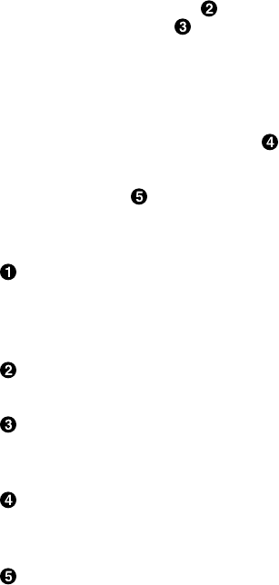
Example 7–1 (Cont.) Displaying Catalogs and Schemas
SQL> --
SQL> -- Display catalogs:
SQL> --
SQL> SHOW CATALOGS
Catalogs in database with filename corporate_data
ADMINISTRATION
RDB$CATALOG
SQL> --
SQL> -- Display schemas:
SQL> --
SQL> SHOW SCHEMAS
Schemas in database with filename corporate_data
ADMINISTRATION.ACCOUNTING
ADMINISTRATION.PERSONNEL
ADMINISTRATION.RECRUITING
RDB$SCHEMA
The following callouts are keyed to Example 7–1:
Your position after attachment to the database is at the top level. This is
indicated by RDB$CATALOG and the schema name as the system user
name. If this schema has not been previously created, it does not actually
exist. It is used only as a starting point.
Only one catalog, named ADMINISTRATION, has been created for this
database.
RDB$CATALOG is the default system catalog that is always created in
multischema databases. This catalog must always be present and is used if
schemas are created and not assigned to any user-defined catalog.
Three schemas; ACCOUNTING, PERSONNEL, and RECRUITING have
been created under the ADMINISTRATION catalog. The periods are used
to separate naming levels.
RDB$SCHEMA is the system default schema and is used to contain the
system tables. It will also be used if a single-schema database is altered to
become a multischema database, and will contain database elements such
as tables and views. It is not prefixed with a catalog name because it is in
the default catalog.
Using Multischema Databases 7–5

Example 7–2 shows how to display tables.
Example 7–2 Displaying Database Tables
SQL> --
SQL> -- Display tables:
SQL> --
SQL> SHOW TABLES
User tables in database with filename corporate_data
ADMINISTRATION.ACCOUNTING.DAILY_HOURS
ADMINISTRATION.ACCOUNTING.DEPARTMENTS
ADMINISTRATION.ACCOUNTING.PAYROLL
ADMINISTRATION.ACCOUNTING.WORK_STATUS
ADMINISTRATION.PERSONNEL.CURRENT_INFO
A view.
ADMINISTRATION.PERSONNEL.CURRENT_JOB
A view.
ADMINISTRATION.PERSONNEL.CURRENT_SALARY
A view.
ADMINISTRATION.PERSONNEL.DEPARTMENTS
ADMINISTRATION.PERSONNEL.EMPLOYEES
ADMINISTRATION.PERSONNEL.HOURLY_HISTORY
ADMINISTRATION.PERSONNEL.JOB_HISTORY
ADMINISTRATION.PERSONNEL.REVIEW_DATE
A view.
ADMINISTRATION.PERSONNEL.SALARY_HISTORY
ADMINISTRATION.RECRUITING.CANDIDATES
ADMINISTRATION.RECRUITING.COLLEGES
ADMINISTRATION.RECRUITING.DEGREES
ADMINISTRATION.RECRUITING.RESUMES
The following callouts are keyed to Example 7–2:
The SHOW TABLES statement issued at the default level catalog and
schema displays the three-level naming convention used to identify tables
in the multischema database.
Database elements, such as tables, can have identical names but must be
placed in separate schemas.
Example 7–3 shows how to display views.
7–6 Using Multischema Databases

Example 7–3 Displaying Database Views
SQL> SHOW VIEWS
User tables in database with filename corporate_data
ADMINISTRATION.PERSONNEL.CURRENT_INFO
A view.
ADMINISTRATION.PERSONNEL.CURRENT_JOB
A view.
ADMINISTRATION.PERSONNEL.CURRENT_SALARY
A view.
ADMINISTRATION.PERSONNEL.REVIEW_DATE
A view.
7.4.1 Displaying Specific Schema Elements
To display elements from specific schemas, use the SHOW statement with the
name of the element (see Table 7–2).
Table 7–2 Using the SHOW Statement to Display Schema Elements
To Display . . . Use the Statement . . .
One table SHOW TABLE table_name
One element of one
table, such as column names
SHOW TABLE (item) table_name
One view SHOW VIEW view_name
One domain SHOW DOMAIN domain_name
All indexes defined on one table SHOW INDEXES ON table_name
SHOW TABLES (INDEXES)
table_name
One index SHOW INDEX index_name
7.4.2 Using the SHOW Statement with a Full Element Name
Example 7–4 shows how to reference database elements using fully qualified
names.
Using Multischema Databases 7–7

Example 7–4 Specifying Full Element Names
SQL> --
SQL> -- Show the current position in the database:
SQL> --
SQL> SHOW DEFAULT
Default alias is RDB$DBHANDLE
Default catalog name is RDB$CATALOG
Default schema name is smith
SQL> SHOW TABLE (COLUMNS) COLLEGES
%SQL-F-SCHNOTDEF, Schema smith is not defined
SQL> SHOW TABLE (COLUMNS) ADMINISTRATION.RECRUITING.COLLEGES
Information for table ADMINISTRATION.RECRUITING.COLLEGES
Stored name is COLLEGES
Columns for table ADMINISTRATION.RECRUITING.COLLEGES:
Column Name Data Type Domain
----------- --------- ------
COLLEGE_CODE CHAR(4) ADMINISTRATION.PERSONNEL.CODE
Primary Key constraint ADMINISTRATION.RECRUITING.COLLEGES_PRIMARY_COLLEGE_CODE
COLLEGE_NAME CHAR(20) ADMINISTRATION.PERSONNEL.NAME
CITY CHAR(20) ADMINISTRATION.PERSONNEL.NAME
STATE CHAR(4) ADMINISTRATION.PERSONNEL.STATE_CODE
ZIP_CODE CHAR(5) ADMINISTRATION.PERSONNEL.POSTAL_CODE
The following callouts are keyed to Example 7–4:
An error occurs because an invalid schema is specified by default. This
schema does not exist.
Because you are positioned at the top level after attaching to the database,
the fully qualified element name must be used.
7.4.3 Using the SET Statement to Access a Specific Catalog and Schema
When you first attach to a multischema database, your default catalog is
RDB$CATALOG and your default schema is your system user name. On
OpenVMS it appears in uppercase type; on Digital UNIX it appears in
lowercase type. All examples in this chapter display the OpenVMS convention.
To work within a specific catalog and schema, you must specify these defaults
by using the SET statement, as shown in Example 7–5.
7–8 Using Multischema Databases

Example 7–5 Setting Access to a Specific Catalog and Schema
SQL> --
SQL> -- Attach to the corporate_data database
SQL> -- and display the default catalog and schema:
SQL> --
SQL> ATTACH ’FILENAME corporate_data’;
SQL> SHOW DEFAULT
Default alias is RDB$DBHANDLE
Default catalog name is RDB$CATALOG
Default schema name is smith
SQL> --
SQL> -- Set default access to the ADMINISTRATION
SQL> -- catalog and PERSONNEL schema:
SQL> --
SQL> SET CATALOG ’ADMINISTRATION’;
SQL> SET SCHEMA ’PERSONNEL’;
SQL> SHOW TABLE EMPLOYEES
Information for table EMPLOYEES
Stored name is EMPLOYEES
Columns for table EMPLOYEES:
Column Name Data Type Domain
----------- --------- ------
EMPLOYEE_ID CHAR(5) ID
Primary Key constraint EMPLOYEES_PRIMARY_EMPLOYEE_ID
LAST_NAME CHAR(20) NAME
FIRST_NAME CHAR(20) NAME
MIDDLE_INITIAL CHAR(1) MIDDLE_INITIAL
ADDRESS_DATA_1 CHAR(25) ADDRESS_LINE
ADDRESS_DATA_2 CHAR(25) ADDRESS_LINE
CITY CHAR(20) NAME
STATE CHAR(4) STATE_CODE
ZIP_CODE CHAR(5) POSTAL_CODE
SEX CHAR(1)
BIRTHDAY DATE ANSI
STATUS CHAR(1) STATUS_CODE
.
.
.
The following callout is keyed to Example 7–5:
The SET statement is used to set up the default catalog and schema for the
session. The catalog and schema specified become the default. This saves
you from having to type in the full element name every time. Later you
can change these settings by issuing another SET statement.
Using Multischema Databases 7–9

7.4.4 Setting a New Default Schema
To view information on tables in other schemas, the current default schema
selection must be changed, as shown in Example 7–6.
Example 7–6 Changing the Default Schema
SQL> SHOW DEFAULT
Default alias is RDB$DBHANDLE
Default catalog name is ADMINISTRATION
Default schema name is PERSONNEL
SQL> SHOW TABLE PAYROLL
No tables found
SQL> SET SCHEMA ’ACCOUNTING’;
SQL> SHOW DEFAULT
Default alias is RDB$DBHANDLE
Default catalog name is ADMINISTRATION
Default schema name is ACCOUNTING
SQL> SHOW TABLE PAYROLL
Information for table PAYROLL
Stored name is PAYROLL
Columns for table PAYROLL:
Column Name Data Type Domain
----------- --------- ------
JOB_CODE CHAR(4) CODE
Primary Key constraint PAYROLL_PRIMARY_JOB_CODE
WAGE_CLASS CHAR(1)
JOB_TITLE CHAR(20) PERSONNEL.NAME
MINIMUM_SALARY INTEGER(2) PERSONNEL.SALARY
MAXIMUM_SALARY INTEGER(2) PERSONNEL.SALARY
Table constraints for PAYROLL:
PAYROLL_PRIMARY_JOB_CODE
Primary Key constraint
Column constraint for PAYROLL.JOB_CODE
Evaluated on COMMIT
Source:
PAYROLL.JOB_CODE PRIMARY KEY
WAGE_CLASS_VALUES
Check constraint
Table constraint for PAYROLL
Evaluated on COMMIT
Source:
CHECK (
WAGE_CLASS in (’1’,’2’,’3’,’4’)
or WAGE_CLASS IS NULL
)
(continued on next page)
7–10 Using Multischema Databases

Example 7–6 (Cont.) Changing the Default Schema
.
.
.
The following callouts are keyed to Example 7–6:
You cannot view this table because it is outside the default schema.
Setting the schema to ACCOUNTING allows you to display the PAYROLL
table.
Example 7–7 shows how to specify elements outside your default schema.
Example 7–7 Displaying Elements from Other Schemas
SQL> SHOW DEFAULT
Default alias is RDB$DBHANDLE
Default catalog name is ADMINISTRATION
Default schema name is ACCOUNTING
SQL> SHOW TABLE PERSONNEL.SALARY_HISTORY
Information for table PERSONNEL.SALARY_HISTORY
Stored name is SALARY_HISTORY
Columns for table PERSONNEL.SALARY_HISTORY:
Column Name Data Type Domain
----------- --------- ------
EMPLOYEE_ID CHAR(5) PERSONNEL.ID
Foreign Key constraint PERSONNEL.SALARY_HISTORY_FOREIGN1
SALARY_AMOUNT INTEGER(2) PERSONNEL.SALARY
SALARY_START DATE ANSI
Not Null constraint PERSONNEL.SALARY_HISTORY_NOT_NULL1
SALARY_END DATE ANSI
Table constraints for PERSONNEL.SALARY_HISTORY:
PERSONNEL.SALARY_HISTORY_FOREIGN1
Foreign Key constraint
Column constraint for PERSONNEL.SALARY_HISTORY.EMPLOYEE_ID
Evaluated on COMMIT
Source:
SALARY_HISTORY.EMPLOYEE_ID REFERENCES EMPLOYEES (EMPLOYEE_ID)
.
.
.
Using Multischema Databases 7–11

The following callout is keyed to Example 7–7:
To display a table from another schema, the schema name must be
specified.
Example 7–8 shows how to display information about views.
Example 7–8 Using the SHOW VIEWS Statement
SQL> SHOW VIEW PERSONNEL.CURRENT_INFO
Information for table CURRENT_INFO
Stored name is CURRENT_INFO
Columns for view CURRENT_INFO:
Column Name Data Type Domain
----------- --------- ------
LAST_NAME CHAR(20)
FIRST_NAME CHAR(20)
ID CHAR(5)
DEPARTMENT CHAR(20)
JOB CHAR(20)
JSTART DATE ANSI
SSTART DATE ANSI
SALARY INTEGER(2)
Source:
SELECT
CJ.LAST_NAME,
CJ.FIRST_NAME,
CJ.EMPLOYEE_ID,
D.DEPARTMENT_NAME,
P.JOB_TITLE,
CJ.JOB_START,
CS.SALARY_START,
CS.SALARY_AMOUNT
FROM ADMINISTRATION.PERSONNEL.CURRENT_JOB CJ,
ADMINISTRATION.PERSONNEL.DEPARTMENTS D,
ADMINISTRATION.ACCOUNTING.PAYROLL p,
ADMINISTRATION.PERSONNEL.CURRENT_SALARY CS
WHERE CJ.DEPARTMENT_CODE = D.DEPARTMENT_CODE
AND CJ.JOB_CODE = P.JOB_CODE
AND CJ.EMPLOYEE_ID = CS.EMPLOYEE_ID
The following callouts are keyed to Example 7–8:
The CURRENT_INFO view is displayed from the PERSONNEL schema.
The view is composed of columns from tables in the ACCOUNTING and
PERSONNEL schemas.
7–12 Using Multischema Databases

7.5 Querying a Multischema Database with SQL
Retrieving data from tables in a multischema database is the same as with a
single-schema database, except that you must identify the catalog and schema,
as shown in Example 7–9.
The first query in the example uses fully qualified column and table names.
The second query uses qualified names only where necessary. The table and
columns in last query need not be qualified, because the catalog and schema
are identified with the SET CATALOG and SET SCHEMA statements prior to
execution of the query.
Example 7–9 Querying Tables in the Default Catalog and Schema
SQL> ATTACH ’FILENAME corporate_data’;
SQL> --
SQL> -- Display name, employee ID, and city for all employees
SQL> -- living in Massachusetts. Fully qualify all table and column names:
SQL> --
SQL> SELECT ADMINISTRATION.PERSONNEL.EMPLOYEES.LAST_NAME,
SQL> ADMINISTRATION.PERSONNEL.EMPLOYEES.EMPLOYEE_ID,
SQL> ADMINISTRATION.PERSONNEL.EMPLOYEES.CITY FROM
SQL> ADMINISTRATION.PERSONNEL.EMPLOYEES
SQL> WHERE ADMINISTRATION.PERSONNEL.EMPLOYEES.STATE = ’MA’;
LAST_NAME EMPLOYEE_ID CITY
Myotte 00174 Bennington
Siciliano 00175 Farmington
Pfeiffer 00191 Marlborough
Gutierrez 00211 Farmington
Harrison 00228 Boston
McElroy 00232 Cambridge
Rodrigo 00249 Bennington
Mistretta 00415 Bennington
MacDonald 00435 Marlborough
9 rows selected
SQL> --
SQL> -- Now perform the same query, but use fully qualified
SQL> -- table and column names only where required:
SQL> --
SQL> SELECT LAST_NAME, EMPLOYEE_ID, CITY FROM
SQL> ADMINISTRATION.PERSONNEL.EMPLOYEES
SQL> WHERE STATE = ’MA’;
LAST_NAME EMPLOYEE_ID CITY
Myotte 00174 Bennington
Siciliano 00175 Farmington
Pfeiffer 00191 Marlborough
Gutierrez 00211 Farmington
(continued on next page)
Using Multischema Databases 7–13

Example 7–9 (Cont.) Querying Tables in the Default Catalog and Schema
Harrison 00228 Boston
McElroy 00232 Cambridge
Rodrigo 00249 Bennington
Mistretta 00415 Bennington
MacDonald 00435 Marlborough
9 rows selected
SQL> --
SQL> -- Last, perform the same query, but identify the catalog and schema
SQL> -- first so that the table name need not be fully
SQL> -- qualified.
SQL> --
SQL> SET CATALOG ’ADMINISTRATION’;
SQL> SET SCHEMA ’PERSONNEL’;
SQL> --
SQL> -- Because the EMPLOYEES table is in the default schema, no
SQL> -- explicit schema name is required:
SQL> --
SQL> SELECT LAST_NAME, EMPLOYEE_ID, CITY
cont> FROM EMPLOYEES
cont> WHERE STATE = ’MA’;
LAST_NAME EMPLOYEE_ID CITY
Myotte 00174 Bennington
Siciliano 00175 Farmington
Pfeiffer 00191 Marlborough
Gutierrez 00211 Farmington
Harrison 00228 Boston
McElroy 00232 Cambridge
Rodrigo 00249 Bennington
Mistretta 00415 Bennington
MacDonald 00435 Marlborough
9 rows selected
The following callouts are keyed to Example 7–9:
In this query, although not required, each table and column name is fully
qualified.
In this query, only the table name needs to be fully qualified because the
columns are all part of the ADMINISTRATION.PERSONNEL.EMPLOYEES
table.
The SET statement establishes the default catalog and schema.
No explicit catalog and schema names are required in this query because
the EMPLOYEES table is in the default catalog and schema.
7–14 Using Multischema Databases

Example 7–10 shows how to query tables outside the default schema.
Example 7–10 Querying Tables in Other Schemas
SQL> SHOW DEFAULT
Default alias is RDB$DBHANDLE
Default catalog name is ADMINISTRATION
Default schema name is PERSONNEL
SQL> --
SQL> -- Display candidates’ names and status:
SQL> --
SQL> SELECT LAST_NAME, FIRST_NAME, CANDIDATE_STATUS
cont> FROM RECRUITING.CANDIDATES;
LAST_NAME FIRST_NAME CANDIDATE_STATUS
Wilson Oscar N
Schwartz Trixie N
Boswick Fred N
3 rows selected
The following callout is keyed to Example 7–10:
When accessing tables in other schemas or catalogs, you must add the
names of those elements to the table name. To access the CANDIDATE_
STATUS table, you must add the RECRUITING schema name.
7.5.1 Joining Tables in a Multischema Database
Example 7–11 shows how to join tables in the same schema.
Example 7–11 Joining Tables in the Same Schema
SQL> --
SQL> SHOW DEFAULT
Default alias is RDB$DBHANDLE
Default catalog name is ADMINISTRATION
Default schema name is PERSONNEL
(continued on next page)
Using Multischema Databases 7–15

Example 7–11 (Cont.) Joining Tables in the Same Schema
SQL> --
SQL> -- Display current salaries of all employees:
SQL> --
SQL> SELECT LAST_NAME, FIRST_NAME, SALARY_AMOUNT
cont> FROM EMPLOYEES AS E, SALARY_HISTORY AS SH
cont> WHERE E.EMPLOYEE_ID = SH.EMPLOYEE_ID
cont> AND SALARY_END IS NULL;
E.LAST_NAME E.FIRST_NAME SH.SALARY_AMOUNT
Toliver Alvin $51,712.00
Smith Terry $11,676.00
Dietrich Rick $18,497.00
Kilpatrick Janet $17,510.00
Nash Norman $52,254.00
Gray Susan $30,880.00
Wood Brian $10,664.00
D’Amico Aruwa $24,064.00
Peters Janis $55,413.00
.
.
.
Silver Glenn $12,350.00
Stornelli James $52,639.00
Belliveau Paul $54,649.00
Lapointe Jo Ann $10,329.00
Crain Jesse $93,340.00
Lapointe Hope $57,410.00
Andriola Leslie $50,424.00
Dement Alvin $57,597.00
Mistretta Kathleen $86,124.00
Ames Louie $26,743.00
Blount Peter $63,080.00
MacDonald Johanna $84,147.00
Herbener James $52,000.00
100 rows selected
The following callout is keyed to Example 7–11:
Joining tables in the same catalog and schema requires no special naming.
Example 7–12 shows how to join tables across schemas.
7–16 Using Multischema Databases

Example 7–12 Joining Tables Across Schemas
SQL> SHOW DEFAULT
Default alias is RDB$DBHANDLE
Default catalog name is ADMINISTRATION
Default schema name is PERSONNEL
SQL> --
SQL> -- Display employee names and degrees earned:
SQL> --
SQL> SELECT LAST_NAME, FIRST_NAME, DEGREE, DEGREE_FIELD
cont> FROM EMPLOYEES AS E, RECRUITING.DEGREES AS D
cont> WHERE E.EMPLOYEE_ID = D.EMPLOYEE_ID;
E.LAST_NAME E.FIRST_NAME D.DEGREE D.DEGREE_FIELD
Toliver Alvin MA Applied Math
Toliver Alvin PhD Statistics
Smith Terry BA Arts
Dietrich Rick BA Arts
Dietrich Rick PhD Applied Math
Kilpatrick Janet BA Arts
Kilpatrick Janet MA Applied Math
Nash Norman MA Applied Math
Nash Norman PhD Applied Math
Gray Susan BA Arts
Gray Susan PhD Applied Math
Wood Brian BA Arts
D’Amico Aruwa MA Applied Math
D’Amico Aruwa MA Elect. Engrg.
Peters Janis BA Arts
.
.
.
MacDonald Johanna PhD Business Admin
Herbener James BA Arts
Herbener James MA Business Admin
165 rows selected
The following callout is keyed to Example 7–12:
Cross schema joins require schema and catalog names when necessary.
7.5.2 Using an SQL Command File to Set the Default Catalog and Schema
If you work with one catalog and schema most of the time, you might want to
place the SET statements in a file, as shown in Example 7–13.
You might also want to make this file your SQL initialization file. See
Section 1.8.6 or Section 2.8.6 for information on how to set up an SQL
initialization file on OpenVMS or Digital UNIX, respectively.
Using Multischema Databases 7–17
Example 7–13 Command File Content: start_multi.sql
SET NOVERIFY
--
PRINT ’Attaching to the corporate_data database...’;
--
ATTACH ’FILENAME corporate_data’;
--
SET CATALOG ’ADMINISTRATION’;
--
SET SCHEMA ’PERSONNEL’;
--
SHOW DEFAULT
The following example shows how to run the command file:
SQL> @START_MULTI
Attaching to the corporate_data database...
Default alias is RDB$DBHANDLE
Default catalog name is ADMINISTRATION
Default schema name is PERSONNEL
7.6 Multischema Access Modes
Sometimes it is necessary to access a multischema database with the
multischema option turned off. Some typical reasons are:
• A single-schema database was altered to become multischema, and
application programs containing unmodified SQL code are expected to
access the database.
• You are using a layered software product that does not support
multischema naming to access the database.
To turn off the multischema attribute of a database, use the MULTISCHEMA
IS OFF option of the ATTACH statement.
7–18 Using Multischema Databases

The general syntax of the statement is:
Syntax ATTACH ’FILENAME database-name MULTISCHEMA IS OFF’;
7.6.1 Multischema Database Element Naming
With the multischema attribute on, each database element is accessed using
its fully qualified name. A fully qualified name is also known as the element’s
SQL name. Each multischema element also has a name that allows it to
be accessed when multischema mode has been turned off. This is called the
element’s stored name.
Example 7–14 shows how to display SQL names for tables in a multischema
database.
Example 7–14 Displaying SQL Names for Database Elements
SQL> --
SQL> -- Display tables in multischema mode.
SQL> -- Two tables have the name ’DEPARTMENTS’.
SQL> --
SQL> ATTACH ’FILENAME corporate_data’;
SQL> SHOW TABLES
User tables in database with filename corporate_data
ADMINISTRATION.ACCOUNTING.DAILY_HOURS
ADMINISTRATION.ACCOUNTING.DEPARTMENTS
ADMINISTRATION.ACCOUNTING.PAYROLL
ADMINISTRATION.ACCOUNTING.WORK_STATUS
ADMINISTRATION.PERSONNEL.CURRENT_INFO
A view.
ADMINISTRATION.PERSONNEL.CURRENT_JOB
A view.
ADMINISTRATION.PERSONNEL.CURRENT_SALARY
A view.
ADMINISTRATION.PERSONNEL.DEPARTMENTS
ADMINISTRATION.PERSONNEL.EMPLOYEES
ADMINISTRATION.PERSONNEL.HOURLY_HISTORY
ADMINISTRATION.PERSONNEL.JOB_HISTORY
ADMINISTRATION.PERSONNEL.REVIEW_DATE
A view.
ADMINISTRATION.PERSONNEL.SALARY_HISTORY
ADMINISTRATION.RECRUITING.CANDIDATES
ADMINISTRATION.RECRUITING.COLLEGES
(continued on next page)
Using Multischema Databases 7–19

Example 7–14 (Cont.) Displaying SQL Names for Database Elements
ADMINISTRATION.RECRUITING.DEGREES
ADMINISTRATION.RECRUITING.RESUMES
SQL> DISCONNECT DEFAULT;
The following callouts are keyed to Example 7–14:
A table in the ACCOUNTING schema has the name DEPARTMENTS.
A table in the PERSONNEL schema also has the name DEPARTMENTS.
When multischema mode is on, access to these tables must be qualified
using the schema name.
7.6.2 Assigning Stored Names
Stored names for database elements can be assigned explicitly by the creator
of the element, or Oracle Rdb will assign a default stored name, as shown in
Example 7–15.
Example 7–15 Displaying Stored Table Names
SQL> --
SQL> -- Attach to the database with multischema mode off.
SQL> -- The two ’DEPARTMENTS’ tables are shown with their
SQL> -- default stored names.
SQL> --
SQL> ATTACH ’FILENAME corporate_data MULTISCHEMA IS OFF’;
(continued on next page)
7–20 Using Multischema Databases

Example 7–15 (Cont.) Displaying Stored Table Names
SQL> SHOW TABLES
User tables in database with filename corporate_data
CANDIDATES
COLLEGES
CURRENT_INFO A view.
CURRENT_JOB A view.
CURRENT_SALARY A view.
DAILY_HOURS
DEGREES
DEPARTMENTS
DEPARTMENTS1
EMPLOYEES
HOURLY_HISTORY
JOB_HISTORY
PAYROLL
RESUMES
REVIEW_DATE A view.
SALARY_HISTORY
WORK_STATUS
The following callouts are keyed to Example 7–15:
DEPARTMENTS is the default name assigned to this table by Oracle Rdb.
The creator of the database has the option of assigning unique stored
names to elements but, in this case, that was not done. Because it was the
first instance of the table name DEPARTMENTS created, it received this
name.
DEPARTMENTS1 is also the default name assigned to this table by Oracle
Rdb. Because it was the second instance created, the number 1 was added
to its name to distinguish it from the first instance of the DEPARTMENTS
table. If DEPARTMENTS was used again, it would receive the stored
name DEPARTMENTS2 by default, and so on.
Reference Reading
For a more detailed discussion of this topic, see the section about
names in multischema databases in the Oracle Rdb7 SQL Reference
Manual.
Using Multischema Databases 7–21

7.6.3 Matching SQL Names to Stored Names
As an application developer, you may have to match a table’s SQL name to its
stored name. This can be difficult if two or more tables have identical SQL
names.
SQL names can be matched to stored names using the following two methods:
• Use the SHOW statement in multischema mode.
• Use the system tables to match the stored name to the SQL name.
7.6.3.1 Using the SHOW Statement to Match SQL Names to Stored Names
Example 7–16 shows how to use the SHOW statement to display a stored table
name.
Example 7–16 Using the SHOW Statement to Display Stored Names
SQL> --
SQL> -- Attach to the corporate_data database
SQL> -- and display the DEPARTMENTS table:
SQL> --
SQL> ATTACH ’FILENAME corporate_data’;
SQL> SET CATALOG ’ADMINISTRATION’;
SQL> SET SCHEMA ’PERSONNEL’;
SQL> SHOW DEFAULT
Default alias is RDB$DBHANDLE
Default catalog name is ADMINISTRATION
Default schema name is PERSONNEL
SQL> SHOW TABLE DEPARTMENTS
Information for table DEPARTMENTS
Stored name is DEPARTMENTS
Columns for table DEPARTMENTS:
Column Name Data Type Domain
----------- --------- ------
DEPARTMENT_CODE CHAR(4) CODE
Primary Key constraint DEPARTMENTS_PRIMARY1
DEPARTMENT_NAME CHAR(20) NAME
Table constraints for DEPARTMENTS:
DEPARTMENTS_PRIMARY1
.
.
.
The following callout is keyed to Example 7–16:
The stored name is given here, and it may be practical to determine stored
names this way for a database with few duplicates. If the database has
7–22 Using Multischema Databases
many duplicate names, however, you can use the system tables method of
determining stored names, as shown in Section 7.6.3.2.
7.6.3.2 Using the System Tables to Match SQL Names to Stored Names
You can query the system tables to map SQL names to stored names.
Example 7–17 shows how to display the system tables for the corporate_
data database.
Example 7–17 Displaying System Tables
SQL> SHOW SYSTEM TABLES
System tables in database with filename corporate_data
RDB$CATALOG.RDB$SCHEMA.RDB$CATALOG_SCHEMA
RDB$CATALOG.RDB$SCHEMA.RDB$COLLATIONS
RDB$CATALOG.RDB$SCHEMA.RDB$CONSTRAINTS
RDB$CATALOG.RDB$SCHEMA.RDB$CONSTRAINT_RELATIONS
RDB$CATALOG.RDB$SCHEMA.RDB$DATABASE
RDB$CATALOG.RDB$SCHEMA.RDB$FIELDS
RDB$CATALOG.RDB$SCHEMA.RDB$FIELD_VERSIONS
RDB$CATALOG.RDB$SCHEMA.RDB$INDEX_SEGMENTS
RDB$CATALOG.RDB$SCHEMA.RDB$INDICES
RDB$CATALOG.RDB$SCHEMA.RDB$INTERRELATIONS
RDB$CATALOG.RDB$SCHEMA.RDB$MODULES
RDB$CATALOG.RDB$SCHEMA.RDB$PARAMETERS
RDB$CATALOG.RDB$SCHEMA.RDB$PRIVILEGES
RDB$CATALOG.RDB$SCHEMA.RDB$QUERY_OUTLINES
RDB$CATALOG.RDB$SCHEMA.RDB$RELATIONS
RDB$CATALOG.RDB$SCHEMA.RDB$RELATION_CONSTRAINTS
RDB$CATALOG.RDB$SCHEMA.RDB$RELATION_CONSTRAINT_FLDS
RDB$CATALOG.RDB$SCHEMA.RDB$RELATION_FIELDS
RDB$CATALOG.RDB$SCHEMA.RDB$ROUTINES
RDB$CATALOG.RDB$SCHEMA.RDB$STORAGE_MAPS
RDB$CATALOG.RDB$SCHEMA.RDB$STORAGE_MAP_AREAS
RDB$CATALOG.RDB$SCHEMA.RDB$SYNONYMS
RDB$CATALOG.RDB$SCHEMA.RDB$TRIGGERS
RDB$CATALOG.RDB$SCHEMA.RDB$VIEW_RELATIONS
RDB$CATALOG.RDB$SCHEMA.RDBVMS$CATALOG_SCHEMA
A view.
RDB$CATALOG.RDB$SCHEMA.RDBVMS$COLLATIONS A view.
RDB$CATALOG.RDB$SCHEMA.RDBVMS$INTERRELATIONS
A view.
RDB$CATALOG.RDB$SCHEMA.RDBVMS$PRIVILEGES A view.
RDB$CATALOG.RDB$SCHEMA.RDBVMS$RELATION_CONSTRAINTS
A view.
RDB$CATALOG.RDB$SCHEMA.RDBVMS$RELATION_CONSTRAINT_FLDS
A view.
(continued on next page)
Using Multischema Databases 7–23

Example 7–17 (Cont.) Displaying System Tables
RDB$CATALOG.RDB$SCHEMA.RDBVMS$STORAGE_MAPS A view.
RDB$CATALOG.RDB$SCHEMA.RDBVMS$STORAGE_MAP_AREAS
A view.
RDB$CATALOG.RDB$SCHEMA.RDBVMS$SYNONYMS A view.
RDB$CATALOG.RDB$SCHEMA.RDBVMS$TRIGGERS A view.
Use the following steps to match a database table’s SQL name to its stored
name using system tables:
Step Action
1 Display the stored names for tables in the database using the SELECT
statement with system tables. (See Example 7–18.)
2 Translate the stored name to an SQL name and display the schema identifier
for each stored name. (See Example 7–19.)
3 Use the schema identifier to determine the schema name and to display the
catalog identifier. (See Example 7–20.)
4 Use the catalog identifier to determine the catalog name. (See Example 7–21.)
Example 7–18 shows how to display the stored table names.
Example 7–18 Displaying the Stored Names for the Tables in the Database
SQL> --
SQL> -- Attach to the database and set schema to RDB$SCHEMA which
SQL> -- contains the system tables:
SQL> --
SQL> ATTACH ’FILENAME corporate_data’;
SQL> SET SCHEMA ’RDB$SCHEMA’;
(continued on next page)
7–24 Using Multischema Databases

Example 7–18 (Cont.) Displaying the Stored Names for the Tables in the
Database
SQL> --
SQL> -- Display stored names of all user tables and views:
SQL> --
SQL> SELECT RDB$RELATION_NAME FROM RDB$RELATIONS
cont> WHERE RDB$SYSTEM_FLAG = 0;
RDB$RELATION_NAME
EMPLOYEES
DEPARTMENTS
JOB_HISTORY
SALARY_HISTORY
HOURLY_HISTORY
CANDIDATES
RESUMES
COLLEGES
DEGREES
WORK_STATUS
PAYROLL
DEPARTMENTS1
DAILY_HOURS
CURRENT_JOB
CURRENT_SALARY
CURRENT_INFO
REVIEW_DATE
17 rows selected
The following callouts are keyed to Example 7–18:
The attach to the database is in multischema mode, so the schema must be
set to RDB$SCHEMA to access the system tables.
Display stored names for tables and views that are in the database.
User tables and views have 0 assigned as an indicator value in
RDB$SYSTEM_FLAG.
Example 7–19 shows how to match a stored name to a schema ID.
Using Multischema Databases 7–25

Example 7–19 Finding the Table’s SQL Name and Schema ID
SQL> --
SQL> -- Query RDBVMS$SYNONYMS system table to link the SQL name
SQL> -- to the stored name and find out the schema ID number:
SQL> --
SQL> SELECT RDBVMS$USER_VISIBLE_NAME, RDBVMS$SCHEMA_ID
cont> FROM RDBVMS$SYNONYMS
cont> WHERE RDBVMS$STORED_NAME=’DEPARTMENTS’
cont> AND RDBVMS$OBJECT_TYPE=31;
RDBVMS$USER_VISIBLE_NAME RDBVMS$SCHEMA_ID
DEPARTMENTS 2
1 row selected
SQL> --
SQL> --
SQL> SELECT RDBVMS$USER_VISIBLE_NAME, RDBVMS$SCHEMA_ID
cont> FROM RDBVMS$SYNONYMS
cont> WHERE RDBVMS$STORED_NAME=’DEPARTMENTS1’
cont> AND RDBVMS$OBJECT_TYPE=31;
RDBVMS$USER_VISIBLE_NAME RDBVMS$SCHEMA_ID
DEPARTMENTS 4
1 row selected
The following callouts are keyed to Example 7–19:
The RDBVMS$SYNONYMS system table connects the stored name of a
table to its SQL name. The RDBVMS$USER_VISIBLE_NAME column
contains the SQL name of the table. The RDBVMS$SCHEMA_ID column
contains the number used to identify its schema.
The RDBVMS$STORED_NAME column contains the stored name of the
table.
Value 31 refers to a table. Other database elements are identified by other
values.
Both tables have the same SQL name but different stored names because
Oracle Rdb requires that all database elements of the same type have unique
names. Given the rules for schema elements within a multischema database,
because both tables have the same SQL name, they must exist in different
schemas (as the different schema identifiers for both indicate).
Example 7–20 shows how to use the schema identifier to determine the schema
name and its catalog identifier.
7–26 Using Multischema Databases

Example 7–20 Finding the Schema Name and Identifying the Parent Catalog
SQL> --
SQL> -- Use the schema identifier to get the schema name
SQL> -- and parent catalog ID:
SQL> --
SQL> SELECT RDBVMS$CATALOG_SCHEMA_ID,
cont> RDBVMS$CATALOG_SCHEMA_NAME,
cont> RDBVMS$PARENT_ID
cont> FROM RDBVMS$CATALOG_SCHEMA
cont> WHERE RDBVMS$CATALOG_SCHEMA_ID > 0;
RDBVMS$CATALOG_SCHEMA_ID RDBVMS$CATALOG_SCHEMA_NAME RDBVMS$PARENT_ID
1 RDB$SCHEMA -1
2 PERSONNEL -2
3 RECRUITING -2
4 ACCOUNTING -2
4 rows selected
SQL>
The following callouts are keyed to Example 7–20:
This column provides the schema identifier. It matches the
RDBVMS$SCHEMA_ID column from the RDBVMS$SYNONYMS system
table.
This column provides the schema name.
This column provides the ID number of the catalog that this schema
belongs to.
This system table contains the name and definition of each SQL catalog
and schema in this database.
Schemas have ID numbers beginning at 1 and increasing. This query
condition ensures that only schemas will be displayed.
The table with the stored name DEPARTMENTS and the schema identifier of
2 is contained in the schema called PERSONNEL. The table with the stored
name DEPARTMENTS1 and the schema identifier of 4 is contained in the
schema called ACCOUNTING.
The values displayed under the RDBVMS$PARENT_ID column are the parent
catalog identifiers for the schemas displayed under the RDBVMS$CATALOG_
SCHEMA_NAME column. The parent identifiers are the same for both the
PERSONNEL and ACCOUNTING schemas. This indicates that both schemas
reside in the same catalog.
Using Multischema Databases 7–27

Example 7–21 shows how to use the catalog identifier to find the catalog
name.
Example 7–21 Displaying the Catalog Identifier and Name
SQL> --
SQL> -- Use the schema parent identifier to determine catalog name:
SQL> --
SQL> SELECT RDBVMS$CATALOG_SCHEMA_ID,
cont> RDBVMS$CATALOG_SCHEMA_NAME,
cont> RDBVMS$PARENT_ID
cont> FROM RDBVMS$CATALOG_SCHEMA
cont> WHERE RDBVMS$CATALOG_SCHEMA_ID < 0;
RDBVMS$CATALOG_SCHEMA_ID RDBVMS$CATALOG_SCHEMA_NAME RDBVMS$PARENT_ID
-1 RDB$CATALOG 0
-2 ADMINISTRATION 0
2 rows selected
The following callouts are keyed to Example 7–21:
Values of less than zero indicate that you are searching for the catalog
identifiers.
The RDBVMS$CATALOG_SCHEMA_NAME column displays the catalogs
in this database.
The corporate_data database contains two catalogs; the default database
RDB$CATALOG catalog with the catalog identifier of , and the
ADMINISTRATION catalog with the catalog identifier of . Because the
schemas PERSONNEL and ACCOUNTING belong to a catalog with an
identifier equal to , you know that the catalog’s name is ADMINISTRATION.
Thus, the table with the stored name of DEPARTMENTS corresponds to the
table named ADMINISTRATION.PERSONNEL.DEPARTMENTS.
The table with the stored name of DEPARTMENTS1 corresponds to the table
named ADMINISTRATION.ACCOUNTING.DEPARTMENTS.
7–28 Using Multischema Databases

8
Using Date-Time Data Types
SQL includes a set of date-time data types and functions that allow you to
manipulate date and time data. By using these data types, functions, and
arithmetic operations you can:
• Store and query many types of date-time data
• Extract and process individual fields within a date-time data type
• Convert date-time data types to other data types for arithmetic
manipulation and display
• Perform date-time arithmetic operations using SQL that cannot be
performed by using high-level languages
This chapter provides introductory information about date-time data types and
built-in functions.
Reference Reading
For more information about using date-time data types, see the Oracle
Rdb7 SQL Reference Manual.
8.1 Date-Time Data Types and Functions
SQL provides specific data types for expressing dates and times. Table 8–1
provides a list of the data types, their format, and a description of their use.
Using Date-Time Data Types 8–1

Table 8–1 Date-Time Data Types
Data Type Name Format Description
DATE VMS
1
dd-mmm-yyyy hh:mm:ss.cc A timestamp containing
year to second.
DATE ANSI yyyy-nn-dd A date of three fields
specifying year, month,
and day.
TIME
2
hh:mm:ss A time of three fields
specifying hour, minute,
and second.
TIMESTAMP yyyy-nn-dd hh:mm:ss.cc A data type composed of
all date-time fields from
year to second. Prior
to Oracle Rdb V7.0, the
format was yyyy-nn-
dd:hh:mm:ss.cc. This
format will continue to
work. However, replacing
the colon between the day
and the hour with a space
conforms to the SQL92
standard.
YEAR-MONTH INTERVAL
yy-nn A data type that describes
the signed duration
between two dates in
years and months.
DAY-TIME INTERVAL
dd:hh:mm:ss.cc A data type that describes
the signed duration
between two dates in
days to seconds.
1
The DATE data type introduced in Oracle Rdb Version 1.0 is called DATE VMS to distinguish it
from the DATE ANSI data type introduced in Oracle Rdb Version 4.1. The DATE VMS data type
cannot be used in date-time arithmetic.
2
The TIME data type specified without a precision specification defaults to no fractional seconds
precision, namely hh:mm:ss. You must specify TIME(2) for SQL to return fractional seconds
precision in the form hh:mm:ss.cc.
SQL also provides special functions that can be used with date-time data types.
Table 8–2 describes these functions.
8–2 Using Date-Time Data Types

Table 8–2 Date-Time Functions
Function Format Description
CURRENT_DATE yyyy-nn-dd Returns today’s date in
DATE ANSI format.
CURRENT_TIME hh:mm:ss Returns the present time
in TIME format.
CURRENT_TIMESTAMP
1
TIMESTAMP data type
(ANSI) format
yyyy-nn-dd:hh:mm:ss.cc Returns the present date
and time in ANSI format.
CURRENT_TIMESTAMP
1
DATE VMS data type
format
dd-mmm-yyyy hh:mm:ss.cc Returns the present date
and time in DATE VMS
format.
EXTRACT Integer Returns a single
date-time field as an
integer from column
of date type DATE,
TIME, TIMESTAMP,
or INTERVAL.
1
The CURRENT_TIMESTAMP function has two formats. By default, SQL displays or stores
CURRENT_TIMESTAMP in DATE VMS format. If you change the default with the SET
DEFAULT DATE FORMAT statement to ANSI format, SQL displays or stores CURRENT_
TIMESTAMP in ANSI format.
8.1.1 DATE VMS Data Type
Date data types specified in the mf_personnel database are of type DATE VMS
(regardless of whether you are working on an OpenVMS or a Digital UNIX
system). This represents the standard date-time definition prior to Oracle Rdb
V4.1 and is still the default date-time data type for Oracle Rdb databases.
Domains and columns specified as DATE VMS cannot be used in date-time
arithmetic unless they are converted to DATE ANSI using the CAST function.
The date literal format for the DATE VMS data type is basically the same
on Digital UNIX as on OpenVMS. However, the XPG4 date and time services
used on Digital UNIX to support locale-specific month abbreviations do not
support the fractional seconds portion of the time. Therefore, any DATE
VMS text literal that contains fractional seconds is truncated such that the
fractional seconds are zero. For example, DATE VMS expressed as
’10-JUL-
1996 12:34:22.56’
on OpenVMS is expressed as
’10-JUL-1996 12:34:22.00’
on Digital UNIX.
Using Date-Time Data Types 8–3

Digital UNIX applications that require the storage of text literals with 10ths
and 100ths of seconds should use the SQL TIMESTAMP literal format. For
example:
CAST(TIMESTAMP’1996-07-10 12:34:22.56’ AS DATE VMS)
Examples of conversion using the CAST function are shown in Section 4.13.1
and in Section 8.1.5.
Example 8–1 shows how DATE VMS is specified in the mf_personnel
database.
Example 8–1 DATE VMS Specification
SQL> -- Display the EMPLOYEES table from the mf_personnel database:
SQL> --
SQL> SHOW TABLE EMPLOYEES
Information for table EMPLOYEES
Comment on table EMPLOYEES:
personal information about each employee
Columns for table EMPLOYEES:
Column Name Data Type Domain
----------- --------- ------
EMPLOYEE_ID CHAR(5) ID_DOM
.
.
.
BIRTHDAY DATE VMS DATE_DOM
.
.
.
SQL> --
SQL> -- Display the DATE_DOM definition:
SQL> --
SQL> SHOW DOMAIN DATE_DOM
DATE_DOM DATE VMS
Comment: standard definition for complete dates
Edit String: DD-MMM-YYYY
SQL> --
SQL> -- Display the birthday for employee 00164:
SQL> --
SQL> SELECT BIRTHDAY FROM EMPLOYEES
cont> WHERE EMPLOYEE_ID= ’00164’;
BIRTHDAY
28-Mar-1947
1 row selected
8–4 Using Date-Time Data Types

The following callouts are keyed to Example 8–1:
The date domain is defined as DATE VMS using the edit string formatting
clause to force SQL to display the date in the format dd-mmm-yyyy with no
time portion.
When defining columns and domains, the data type for DATE will be
interpreted as DATE VMS unless DATE ANSI is explicitly specified, the
SET DEFAULT DATE FORMAT statement is used, or the SET DIALECT
statement is used to set the default format as DATE ANSI. See the Oracle
Rdb7 SQL Reference Manual for more details on using these statements.
The format includes digits and letters. Note the difference between this
format and DATE ANSI shown in Example 8–2.
8.1.2 DATE ANSI Data Type
DATE ANSI is a distinct data type from DATE VMS. It contains year, month,
and day fields (yyyy-nn-dd).
Example 8–2 shows how DATE ANSI is specified in the corporate_data
database.
Example 8–2 DATE ANSI Specification
SQL> --
SQL> -- Display the EMPLOYEES table from the corporate_data
SQL> -- database:
SQL> --
SQL> SHOW TABLE EMPLOYEES
Information for table EMPLOYEES
Stored name is EMPLOYEES
Columns for table EMPLOYEES:
Column Name Data Type Domain
----------- --------- ------
EMPLOYEE_ID CHAR(5) ID
.
.
.
BIRTHDAY DATE ANSI
STATUS CHAR(1) STATUS_CODE
.
.
.
(continued on next page)
Using Date-Time Data Types 8–5

Example 8–2 (Cont.) DATE ANSI Specification
SQL> --
SQL> -- Display the birthday for employee 00164:
SQL> --
SQL> SELECT BIRTHDAY FROM EMPLOYEES
cont> WHERE EMPLOYEE_ID= ’00164’;
BIRTHDAY
1947-03-28
1 row selected
The following callouts are keyed to Example 8–2:
DATE ANSI is specified for the BIRTHDAY column in the corporate_data
database.
Unlike DATE VMS, DATE ANSI data is displayed in year-to-day format
(yyyy-nn-dd).
8.1.3 TIMESTAMP Data Type
TIMESTAMP contains all of the date and time fields: year, month, day, hour,
minute, second, and fractions of a second.
Example 8–3 shows how a TIMESTAMP is defined in the corporate_data
database.
Example 8–3 TIMESTAMP Specification
SQL> -- Display the DAILY_HOURS table from the
SQL> -- corporate_data database:
SQL> --
SQL> SET CATALOG ’ADMINISTRATION’;
SQL> SET SCHEMA ’ACCOUNTING’;
SQL> SHOW TABLE DAILY_HOURS
Information for table DAILY_HOURS
Stored name is DAILY_HOURS
Columns for table ACCOUNTING.DAILY_HOURS:
Column Name Data Type Domain
----------- --------- ------
EMPLOYEE_ID CHAR(5) PERSONNEL.ID
START_TIME TIMESTAMP(2)
END_TIME TIMESTAMP(2)
(continued on next page)
8–6 Using Date-Time Data Types

Example 8–3 (Cont.) TIMESTAMP Specification
.
.
.
SQL> --
SQL> -- Insert employee starting and ending times:
SQL> --
SQL> INSERT INTO DAILY_HOURS
cont> (EMPLOYEE_ID, START_TIME, END_TIME)
cont> VALUES (’00164’, TIMESTAMP’1992-04-23 07:58:23.16’,
cont> TIMESTAMP’1992-04-23 17:08:15.06’);
1 row inserted
SQL> --
SQL> -- Display start time for employee 00164:
SQL> --
SQL> SELECT EMPLOYEE_ID, START_TIME
cont> FROM DAILY_HOURS
cont> WHERE EMPLOYEE_ID= ’00164’;
EMPLOYEE_ID START_TIME
00164 1992-04-23:07:58:23.16
1 row selected
The following callouts are keyed to Example 8–3:
TIMESTAMP(2) indicates that precision is set to two places to the
right of the decimal point. It was unnecessary to specify this, however,
because TIMESTAMP displays this fractional precision by default. To omit
fractional seconds specify TIMESTAMP(0).
The literal format is used to insert TIMESTAMP values.
The standard display is year-to-second format (yyyy-nn-dd hh:mm:ss.cc).
8.1.4 TIME Data Type
TIME specifies 24-hour military time containing hours, minutes, seconds, and
optionally, fractions of a second fields.
TIME has limited value as a column or domain specification. In Example 8–4,
TIMESTAMP is converted to TIME format. The CAST function is being used
for date-time field conversion.
Using Date-Time Data Types 8–7

Example 8–4 Displaying Data in TIME Format
SQL> -- Display starting time without fractional seconds
SQL> -- for employee 00164:
SQL> --
SQL> SET CATALOG ’ADMINISTRATION’;
SQL> SET SCHEMA ’ACCOUNTING’;
SQL> SELECT CAST(START_TIME AS TIME) AS STARTING_TIME
cont> FROM DAILY_HOURS
cont> WHERE EMPLOYEE_ID= ’00164’;
STARTING_TIME
07:58:23
1 row selected
The following callouts are keyed to Example 8–4:
START_TIME is specified as a TIMESTAMP and CAST is used to convert
it to TIME, which is more readable. TIME(2) could have been specified to
display the fractional seconds.
The format is hours, minutes, and seconds (hh:mm:ss). Data appears with
the column name STARTING_TIME because it was specified as the column
name in the SELECT statement.
8.1.5 INTERVAL Data Type
INTERVAL is used to describe the duration or time between two events.
Intervals fall into two categories: year-month intervals and day-time intervals.
The INTERVAL data type takes qualifiers to specify the contents of the interval
field.
Table 8–3 lists the qualifiers for the two INTERVAL types.
Table 8–3 Interval Qualifiers
Interval Category Interval Qualifiers
YEAR-MONTH YEAR
YEAR TO MONTH
MONTH
DAY-TIME DAY
(continued on next page)
8–8 Using Date-Time Data Types

Table 8–3 (Cont.) Interval Qualifiers
Interval Category Interval Qualifiers
DAY TO HOUR
DAY TO MINUTE
DAY TO SECOND
HOUR
HOUR TO MINUTE
HOUR TO SECOND
MINUTE
MINUTE TO SECOND
SECOND
The two interval categories are essential to any date-time interval calculation
because arithmetic operations are not possible without informing SQL as to
which YEAR-MONTH or DAY-TIME interval result you require. There are two
main reasons why you must communicate this information to SQL and why
the categories are neither compatible nor comparable in any way:
• You cannot convert a YEAR-MONTH interval to a DAY-TIME interval.
For example, you cannot convert a YEAR-MONTH interval of two years
and five months into hours to produce an accurate DAY-TIME interval.
First, you do not know whether or not the year value includes a leap year.
Second, you do not know what months are represented in the five-month
interval. For example, the months from January to May contain a different
number of days than the months from February to June, and this number
would differ depending on the year as well.
• You cannot convert a DAY-TIME interval to a YEAR-MONTH interval.
For example, you cannot convert a DAY-TIME interval of 1000 days into a
YEAR-MONTH interval in months to produce an accurate YEAR-MONTH
interval. The answer depends strictly on when the interval starts in
absolute time.
Using Date-Time Data Types 8–9

8.1.6 Using the INTERVAL Data Type
Example 8–5 shows how INTERVAL is used to define a column in the
corporate_data database.
Example 8–5 INTERVAL Specification
SQL> -- Display the INTERVAL in the DAILY_HOURS table
SQL> -- of the corporate_data database:
SQL> --
SQL> SET CATALOG ’ADMINISTRATION’;
SQL> SET SCHEMA ’ACCOUNTING’;
SQL> SHOW TABLE DAILY_HOURS
Information for table DAILY_HOURS
Stored name is DAILY_HOURS
Columns for table DAILY_HOURS:
Column Name Data Type Domain
----------- --------- ------
EMPLOYEE_ID CHAR(5) PERSONNEL.ID
START_TIME TIMESTAMP(2)
END_TIME TIMESTAMP(2)
HOURS_WORKED INTERVAL
HOUR (2) TO SECOND (2)
Computed: BY (END_TIME - START_TIME) HOUR TO SECOND
SQL> --
SQL> -- Display hours worked for employee number 00164:
SQL> --
SQL> SELECT CAST(START_TIME AS TIME) AS STARTING_TIME,
cont> CAST(END_TIME AS TIME) AS ENDING_TIME, HOURS_WORKED
cont> FROM DAILY_HOURS
cont> WHERE EMPLOYEE_ID = ’00164’;
STARTING_TIME ENDING_TIME HOURS_WORKED
07:58:23 17:08:15 09:09:51.90
1 row selected
The following callouts are keyed to Example 8–5:
HOURS_WORKED is specified as an INTERVAL data type. The
INTERVAL is computed by subtracting the START_TIME from the
END_TIME timestamps. An INTERVAL qualifier must be specified to
determine the result. In this case, HOUR TO SECOND is used to show
hours worked. HOUR(2) indicates the leading field will occupy 2 spaces.
This is also known as leading field precision. SECOND(2) indicates that
fractions of a second will display.
Casting the TIMESTAMP data type as TIME is used to clarify the output
by displaying only the time portion of the timestamps.
8–10 Using Date-Time Data Types

The interval is calculated and displayed as specified by the INTERVAL
qualifier HOUR TO SECOND.
Reference Reading
For a full discussion of INTERVAL qualifiers and precision, see the
date-time data types section of the Oracle Rdb7 SQL Reference Manual.
8.2 Date-Time Data Type Literal Formats
Table 8–4 shows date-time literals and the many permutations of INTERVAL
literals. Precision can be specified for literal fields.
INTERVAL maintains literal formats to accommodate the full range of date-
time combinations. The numbers within single quotes are examples of values
that can be input in INTERVAL format for date-time computations. The
INTERVAL qualifier must be specified to inform SQL how to interpret the
value, and correct separator characters must be included. Note that negative
values can be used for date-time computations.
Table 8–4 Date-Time Data Type Literal Formats
Date-Time Literal Formats Example
DATE ’yyyy-nn-dd’ DATE ’1992-02-04’
TIME ’hh:mm:ss.cc’ TIME ’07:14:21.43’
1
TIMESTAMP ’yyyy-nn-dd hh:mm:ss.cc’
2
TIMESTAMP ’1991-03-12 04:15:20.45’
INTERVAL ’
dd:hh:mm:ss.cc’
3
—–
INTERVAL ’ literal-value’ YEAR INTERVAL ’2’ YEAR
INTERVAL ’ literal-value’ YEAR TO MONTH INTERVAL ’2-01’ YEAR TO MONTH
INTERVAL ’ literal-value’ MONTH INTERVAL ’8’ MONTH
INTERVAL ’ literal-value’ DAY INTERVAL ’07’ DAY
1
The default value for the TIME data type is TIME(0) or TIME with no fractional precision. Thus, the example shows a
TIME literal that requires a TIME(2) data type declaration.
2
Prior to Oracle Rdb V7.0 the day and hour fields were separated with a colon. Beginning in Oracle Rdb V7.0, these
fields can be separated by a space, which conforms to the SQL92 standard. Either format is acceptable to Oracle Rdb
V7.0.
3
This table provides examples for each permutation of the date-time INTERVAL literal qualifiers allowed by the
INTERVAL data type.
(continued on next page)
Using Date-Time Data Types 8–11

Table 8–4 (Cont.) Date-Time Data Type Literal Formats
Date-Time Literal Formats Example
INTERVAL ’ literal-value’ DAY TO HOUR INTERVAL ’14:10’ DAY TO HOUR
INTERVAL ’ literal-value’ DAY TO MINUTE INTERVAL ’+14:13:27’ DAY TO MINUTE
INTERVAL ’ literal-value’ DAY TO SECOND INTERVAL ’–25:11:16:22.51’ DAY TO SECOND
INTERVAL ’ literal-value’ HOUR INTERVAL ’15’ HOUR
INTERVAL ’ literal-value’ HOUR TO MINUTE INTERVAL ’15:33’ HOUR TO MINUTE
INTERVAL ’
literal-value’ HOUR TO SECOND INTERVAL ’22:41:18.25’ HOUR TO SECOND
INTERVAL ’ literal-value’ MINUTE INTERVAL ’39’ MINUTE
INTERVAL ’ literal-value’ MINUTE TO SECOND INTERVAL ’29:16’ MINUTE TO SECOND
INTERVAL ’ literal-value’ SECOND INTERVAL ’43.39’ SECOND
As shown in Table 8–4, you separate each field with special syntax characters.
Each field must be numeric and can contain leading zeros. The seconds field
includes a fractional portion that SQL does not treat as a separate field. SQL
requires that you include a value for each literal field and that the value be
within the valid range for that field. Refer to the Oracle Rdb7 SQL Reference
Manual for information about valid field ranges.
Example 8–6 shows how to use an INTERVAL literal value with a qualifier in
date-time arithmetic.
Example 8–6 Using INTERVAL with the DATE Data Type
SQL> -- Using the corporate_data database, determine
SQL> -- how old Toliver will be five years from today.
SQL> --
SQL> ATTACH ’FILENAME corporate_data’;
SQL> SET CATALOG ’ADMINISTRATION’
SQL> SET SCHEMA ’PERSONNEL’;
8–12 Using Date-Time Data Types

SQL> SELECT EMPLOYEE_ID, LAST_NAME, FIRST_NAME,
cont> ((CURRENT_DATE + INTERVAL’5’ YEAR) - BIRTHDAY)YEAR AS AGE
cont> FROM EMPLOYEES
cont> WHERE EMPLOYEE_ID = ’00164’;
EMPLOYEE_ID LAST_NAME FIRST_NAME AGE
00164 Toliver Alvin 53
1 row selected
The following callout is keyed to Example 8–6:
To add an INTERVAL to a DATE data type, use the literal format.
INTERVAL ’5’ adds five years to CURRENT_DATE. Using INTERVAL
’5-6’ would add five years and six months to CURRENT_DATE.
8.3 Using the EXTRACT Function
The EXTRACT function allows you to access individual fields from a column
of the data type DATE, TIME, TIMESTAMP, or INTERVAL, and returns an
integer. It can also be used with the keyword JULIAN to count the number
of days from the first day of the year, or the keyword WEEKDAY to give an
ordinal number indicating position in the week.
The values that the EXTRACT function can return are:
• YEAR
• MONTH
•DAY
• HOUR
• MINUTE
• SECOND
• WEEKDAY
• JULIAN
The general syntax of the statement is:
Syntax SELECT . . .
EXTRACT (date-time-field FROM extract-source)
FROM . . . ;
Using Date-Time Data Types 8–13

The result of EXTRACT is always a numeric (INTEGER), except for second,
which returns a scaled numeric (INTEGER(2)) value. In addition to the
date-time field names, SQL provides the WEEKDAY and JULIAN keywords.
WEEKDAY returns a number 1 (Monday) through 7 (Sunday), and JULIAN
returns a value of 1 to 365 or 1 to 366. Example 8–7 shows how to use the
EXTRACT function.
Example 8–7 Extracting Date-Time Information
SQL> -- Display the hours worked by employee 00164:
SQL> --
SQL> SET CATALOG ’ADMINISTRATION’;
SQL> SET SCHEMA ’ACCOUNTING’;
SQL> SELECT EXTRACT(YEAR FROM START_TIME) AS YEAR,
cont> EXTRACT(MONTH FROM START_TIME) AS MONTH,
cont> EXTRACT(DAY FROM START_TIME) AS DAY,
cont> EXTRACT(HOUR FROM HOURS_WORKED) AS HOURS
cont> FROM DAILY_HOURS
cont> WHERE EMPLOYEE_ID = ’00164’;
YEAR MONTH DAY HOURS
1992 4 23 9
1 row selected
SQL> --
SQL> -- Display the day of the week from starting time:
SQL> --
SQL> SELECT EXTRACT(WEEKDAY FROM START_TIME) AS WEEK_DAY
cont> FROM ACCOUNTING.DAILY_HOURS
cont> WHERE EMPLOYEE_ID = ’00164’;
WEEK_DAY
4
1 row selected
SQL> --
SQL> -- Display the birthday of employee 00164:
SQL> --
SQL> SET SCHEMA ’PERSONNEL’;
SQL> SELECT BIRTHDAY FROM EMPLOYEES
cont> WHERE EMPLOYEE_ID = ’00164’;
BIRTHDAY
1947-03-28
1 row selected
(continued on next page)
8–14 Using Date-Time Data Types

Example 8–7 (Cont.) Extracting Date-Time Information
SQL> --
SQL> -- Display the birthday as the Julian date:
SQL> --
SQL> SELECT EXTRACT(JULIAN FROM BIRTHDAY) AS JULIAN_DATE
cont> FROM EMPLOYEES
cont> WHERE EMPLOYEE_ID = ’00164’;
JULIAN_DATE
87
1 row selected
The following callouts are keyed to Example 8–7:
The column START_TIME is a timestamp containing YEAR to SECOND
fields. These fields can be extracted individually to give you the
information that you want.
Extract the HOUR field from the INTERVAL HOURS_WORKED.
WEEKDAY is extracted from the timestamp START_TIME. WEEKDAY
is an integer value representing the day of the week. In this case the
5 indicates Friday and the 1 indicates Monday. WEEKDAY can only be
extracted from DATE and TIMESTAMP data types.
The JULIAN keyword is used with the EXTRACT function to return the
number of days from the beginning of the year, in this example 1947, in
which the birthday occurred.
8.4 Rules for Performing Date-Time Arithmetic
You may need to use date-time data type variables and constants in arithmetic
expressions. The legal arithmetic operations that SQL allows are listed in
Table 8–5. Date-time refers to a variable or literal of data type DATE ANSI,
TIME, or TIMESTAMP. INTERVAL refers to the intervals YEAR-MONTH or
DAY-TIME.
Using Date-Time Data Types 8–15

Table 8–5 Valid Arithmetic Operations with Date-Time Data Types
Operand 1 Operator Operand 2 Resulting Data Type
DATE ANSI + TIME TIMESTAMP
date-time – date-time INTERVAL (qualified)
date-time + or – INTERVAL date-time
INTERVAL + or – INTERVAL INTERVAL
INTERVAL * or / numeric INTERVAL
numeric + or – INTERVAL INTERVAL
When an arithmetic operation results in an INTERVAL, a qualifier must be
specified. See Table 8–3 for a full listing of INTERVAL qualifiers. Example 8–8
shows how to specify an INTERVAL qualifier.
Example 8–8 Using CURRENT_DATE and INTERVAL
SQL> -- Find the age of every employee:
SQL> --
SQL> SET CATALOG ’ADMINISTRATION’;
SQL> SET SCHEMA ’PERSONNEL’;
SQL> SELECT EMPLOYEE_ID, LAST_NAME, FIRST_NAME,
cont> (CURRENT_DATE - BIRTHDAY)YEAR AS AGE
cont> FROM EMPLOYEES;
EMPLOYEE_ID LAST_NAME FIRST_NAME AGE
00164 Toliver Alvin 48
00165 Smith Terry 40
00166 Dietrich Rick 41
.
.
.
00471 Herbener James 67
100 rows selected
The following callout is keyed to Example 8–8:
Subtraction of two date-time data types results in an interval that must be
qualified. In this case YEAR is the qualifier.
In Example 8–9, START_TIME must be cast as TIME before it can be
subtracted from CURRENT_TIME. This is because you can only use data types
with similiar fields in date-time arithmetic.
8–16 Using Date-Time Data Types
Example 8–9 Subtracting TIME
SQL> -- How long has Toliver worked today?
SQL> --
SQL> SET CATALOG ’ADMINISTRATION’;
SQL> SET SCHEMA ’ACCOUNTING’;
SQL> SELECT EMPLOYEE_ID,
cont> (CURRENT_TIME - CAST(START_TIME AS TIME)) HOUR TO MINUTE AS HOURS_WORKED
cont> FROM DAILY_HOURS
cont> WHERE EMPLOYEE_ID = ’00164’;
EMPLOYEE_ID HOURS_WORKED
00164 07:29
1 row selected
In Example 8–10, the SUM function is used to add the INTERVAL HOURS_
WORKED to determine the total time on the job for employee 00164. The
result is given as a qualified INTERVAL of hours-to-seconds.
Example 8–10 Using SUM with INTERVAL
SQL> -- How many hours has employee 00164 worked in total?
SQL> --
SQL> SET CATALOG ’ADMINISTRATION’;
SQL> SET SCHEMA ’ACCOUNTING’;
SQL> SELECT SUM(HOURS_WORKED) AS WEEKLY_HOURS
cont> FROM DAILY_HOURS
cont> WHERE EMPLOYEE_ID = ’00164’;
WEEKLY_HOURS
18:58:19.25
1 row selected
Using Date-Time Data Types 8–17

Index
!
See Exclamation point as comment character
%
See Percent sign
*
See Asterisk
<
See Less than operator
<=
See Less than or equal to operator
<>
See Not equal to operator
>
See Greater than operator
>=
See Greater than or equal to operator
_
See Underscore
A
Accessing a database, 1–4, 2–4
Adding a comment, 3–6
Aggregate functions, 4–39
ALL keyword, 4–11, 6–14, 6–15e
Alternative column name
using, 4–5e
AND operator, 4–35
when parentheses delimit condition, 4–38
ANY keyword, 6–14, 6–15e
Ascending value
ordering row in, 4–12
ASC keyword
in ORDER BY clause, 4–12
AS keyword
in select list, 4–13, 6–25
Assigning stored names explicitly, 7–20
Asterisk ( * )
in COUNT function, 4–41
use in SELECT statement, 4–4e, 6–10
use in SHOW TABLE statement, 3–1
ATTACH statement
description, 1–4, 2–4
description for multischema database, 7–3
MULTISCHEMA IS OFF option, 7–19
AVG function, 4–40
returning null value, 4–42
B
BETWEEN predicate, 4–21e
Boolean operator, 4–35
order of precedence, 4–37
truth table, 4–37
Built-in functions, 4–43, 4–44t
C
Cartesian product, 4–58
Case sensitivity
CONTAINING predicate and, 4–26
LIKE predicate and, 4–28
CAST function
converting data types, 4–44, 8–8e, 8–10e
definition of, 4–44
format of, 4–44
using to convert TIME, 8–7
Index–1

Casting
See CAST function
Catalog, 7–2
displaying, 7–4e
setting default, 7–17
Changing a comment, 3–6
CHARACTER_LENGTH function, 4–45
CHAR_LENGTH function, 4–45
Column select expression, 6–4
Command file
See Indirect command file
Command procedure, 1–6
See also SQL command procedure
sqlini.sql initialization file, 2–9, 7–17
SQLINI initialization file, 1–9, 7–17
Comment
adding, 3–6e
adding multistring comments, 3–6e
changing, 3–6
including in an SQL command procedure, 1–6
including in an SQL indirect command file,
2–6
COMMENT ON statement, 3–6
COMMIT statement, 5–2t
Comparison
semantic meaning of, 4–20
Comparison predicates, 4–18, 4–19e
valid data types, 4–18
Computed value
ordering rows by, 4–13
Condition
alternative, 4–35
combined, 4–35
evaluating
order of, 4–37
truth table, 4–37
negated, 4–35
specifying, 4–16
Conditional operator, 4–35
comparing value expression, 4–17
Configuration parameter
SQL_DATABASE, 2–6
Constraints
displaying, 5–24
effects on write operations, 5–23
CONTAINING predicate, 4–26
Controlling interactive session output, 1–7t,
2–7t
Conversion
value expression to lowercase, 4–51
corporate_data database
See Sample database
Correlation name, 4–63
COUNT function, 4–41
returning empty stream, 4–43
using asterisk ( *) in, 4–41
using DISTINCT keyword, 4–41
Counting
row, 4–41
unique column value, 4–41
CREATE VIEW statement, 6–30
Crossing tables, 4–59
CURRENT_DATE function
format, 8–1t
CURRENT_TIME function
format, 8–1t
CURRENT_TIMESTAMP function
formats, 8–1t
CURRENT_TIMESTAMP keyword, 5–19
CURRENT_USER keyword, 5–19
D
Database
defining a default database using
SQL$DATABASE, 1–6
defining a default database using SQL_
DATABASE, 2–6
detaching from, 1–4, 2–4
displaying information about, 3–1
inserting a row in, 5–3
multischema
See Multischema database
DATE ANSI data type
format, 8–1t, 8–5e
when introduced, 8–1t
DATE data type, 8–3
literal format, 8–11t
using with INTERVAL data type, 8–12e
Index–2

Date-time data types, 8–1 to 8–17
arithmetic rules for, 8–15
formats, 8–2t
functions, 8–2t
literal format, 8–3
valid arithmetic operations, 8–15t
DATE VMS data type, 8–3
format, 8–1t, 8–3, 8–4e
when introduced, 8–1t
DCL commands
executing from interactive SQL, 1–5
DEC Language-Sensitive Editor
See DEC LSE editor
DEC LSE editor
description, 1–8
using with EDIT statement, 1–8
DECTPU editor
using with EDIT statement, 1–7
Default catalog
setting, 7–17
Default stored names, 7–20
Default value, 5–7
See also Null value
when inserting a row, 5–9e
DELETE statement, 5–17
Deleting rows, 5–17
Derived table, 6–25, 6–26e
Descending value
ordering row in, 4–12
DESC keyword
in ORDER BY clause, 4–12
Detaching from a database, 1–4, 2–4
DISCONNECT statement, 1–4, 2–4
Displaying domains, 3–3, 8–4e
Displaying indexes, 3–4
Displaying stored names, 7–20e
DISTINCT keyword, 4–9, 4–10e
using in COUNT function, 4–41
Dividing column values, 4–7e
Domains
displaying, 3–3, 8–4e
Double hyphen (--) as comment character, 1–6,
2–6
Duplicate row
eliminating, 4–9
E
Editing SQL statements, 1–8t
Editor
See also EDT editor; DEC LSE editor;
DECTPU editor; vi editor
defining for EDIT statement, 1–7, 2–8
EDITOR environment variable, 2–8
EDIT statement, 1–5, 2–5, 2–8
EDT editor
using with EDIT statement, 1–7
Ending a transaction, 5–2
Equal to operator (=), 4–18
Equijoin, 4–60t
Error
correcting an interactive statement, 1–5, 2–5
ESCAPE keyword, 4–28
Exclamation point (!) as comment character, 1–6
Executing DCL commands
from interactive SQL, 1–5
EXISTS predicate, 6–9e
EXIT statement, 5–2t
Expression
value, 4–6, 4–7e
comparing, 4–17
EXTRACT function
description, 8–13
using, 8–14e
F
FROM clause, 4–2, 4–50, 6–25
Function, 4–39
CAST, 4–44
CHARACTER_LENGTH, 4–45
CHAR_LENGTH, 4–45
date-time, 8–2
EXTRACT, 8–13
interaction with null value, 4–42
LOWER, 4–51
OCTET_LENGTH, 4–45
POSITION, 4–49
Index–3

Function (cont’d)
returning empty stream, 4–42
SUBSTRING, 4–46
TRANSLATE, 4–52
TRIM, 4–47
UPPER, 4–51
G
Greater than operator (>), 4–18
Greater than or equal to operator (>=), 4–18
GROUP BY clause, 4–53, 4–56
H
HAVING clause, 4–56, 6–4
HELP statement, 1–3, 2–3
I
IGNORE CASE keyword, 4–28, 4–29
Implicit join, 4–61
Indexes
displaying, 3–4
Indirect command file
SQL, 2–6
Initialization file
for interactive SQL, 1–9, 2–9
Inner join, 4–64
IN predicate, 4–23, 4–24e, 6–14
INSERT statement, 5–3e
conversion of data type when inserting data,
5–15
copying data from another table, 5–10e
inserting a calculated value, 5–11e
specifying NULL value, 5–9e
Interactive SQL
editing statement, 1–5, 2–5
exiting, 1–3, 2–3
getting started with, 1–1, 2–1
invoking on Digital UNIX, 2–3
invoking with DCL symbol, 1–2
setting up environment, 1–9, 2–9
Interactive SQL command procedure, 1–6
Interactive SQL indirect command file, 2–6
INTERVAL data type, 8–10
addition, 8–12e
formats, 8–1t, 8–8e
literal format, 8–11e
using SUM function with, 8–17e
using to define a column, 8–10e
using with DATE data type, 8–12e
IS NOT NULL predicate, 4–34
IS NULL predicate, 4–21, 4–31
J
Join, 4–58
equijoin, 4–60t
implicit, 4–61
inner, 4–64e
natural, 4–60t, 4–64e, 6–22
outer, 6–22
types of, 4–60t
Joining more than two tables, 4–67e
Joining tables, 4–58, 4–62e
answering reflexive questions, 4–70
in a multischema database, 7–15
using a table as a bridge, 4–68
using explicit join syntax, 4–64, 6–24e
using implicit join syntax, 4–61
JULIAN keyword, 8–13
L
Leading characters
removing, 4–47
Less than operator (<), 4–18
Less than or equal to operator (<=), 4–18
LIKE predicate, 4–27, 4–29t
LIMIT TO clause, 4–15, 4–16e, 6–16e
Logical name
SQL$DATABASE, 1–6
SQL$EDIT, 1–7
SQLINI, 1–9
login.com file
including symbol for interactive SQL, 1–2
logical name to include in, 1–9
Index–4

Lowercase
converting value expression to, 4–51
LOWER function, 4–51
M
MAX function, 4–40
returning null value, 4–42
mf_personnel database
See Sample database
MIN function, 4–40
returning null value, 4–42
Multischema database
access modes, 7–18
assigning stored names, 7–20
attaching to, 7–3
catalog within, 7–2
displaying catalogs and schemas, 7–4e
displaying elements, 7–4
displaying tables, 7–6e
displaying views, 7–7e
element naming, 7–19
joining tables across schemas, 7–15e
matching SQL names to stored element
names, 7–22, 7–23e
overview, 7–1
querying, 7–13e
sample database, 7–1
schema within, 7–2
setting default catalog and schema, 7–8
structure of, 7–2f
Multistring comments, 3–6e
N
Natural join, 4–60t, 4–64e, 6–22
Not equal to operator (<>), 4–18
NOT EXISTS predicate, 6–3, 6–9e
NOT IN predicate, 4–25, 6–16e
NOT operator, 4–35
NOT SINGLE predicate, 6–9
Null value, 4–21, 4–31
interaction with function, 4–42
predicate, 4–18, 4–31
when inserting a row, 5–9e
O
OCTET_LENGTH function, 4–45
ON clause, 4–64
Operator
Boolean
order of precedence, 4–37
conditional, 4–35
ORDER BY clause, 4–11, 4–12e, 6–16e
ASC keyword, 4–12
DESC keyword, 4–12
specifying column, 4–13
by name, 4–14
by ordinal position in SELECT clause,
4–14
Ordering
of columns, 4–3
rows, 4–11
by ascending value, 4–12
by descending value, 4–12
for processing by function, 4–56
OR operator, 4–35
when parentheses delimit condition, 4–38
Outer joins
overview, 6–22
using to answer a question, 6–24e
P
Parentheses ( )
in search condition, 4–37
Pattern matching
retrieving data by, 4–27
Pattern matching predicate, 4–18, 4–27
Percent sign ( %)
searching for, 4–29
wildcard character in pattern matching, 4–28
personnel database
See Sample database
POSITION function, 4–49
Predicate
See also Boolean operator; Condition;
Conditional operator
definition, 4–16
Index–5

Predicate (cont’d)
EXISTS, 6–9e
IS NULL, 4–21, 4–31
LIKE, 4–27, 4–29t
NOT EXISTS, 6–3, 6–9e
NOT IN, 6–16e
NOT SINGLE, 6–9
number of conditions in, 4–35
quantified, 6–4, 6–14
retrieving data by, 4–17e
SINGLE, 6–9
Q
Quantified predicate, 6–4, 6–14
QUIT statement, 5–2t
R
Range test predicate, 4–18, 4–21
Relational operator
See Conditional operator
Result table, 4–3
Retrieving data
by predicate, 4–17e
eliminating duplicate rows, 4–9
limiting number of rows (LIMIT TO), 4–15
ordering rows, 4–11
selecting
all rows in table (ALL), 4–11
selecting columns, 4–2
specifying
condition, 4–16
ROLLBACK statement, 5–2t, 5–3e
Rows
counting number of, 4–41
deleting, 5–17
inserting, 5–3
ordering, 4–11
updating, 5–11
S
Sample database
assigning a configuration parameter, 2–6
assigning a logical name, 1–6
creating, 1–2t, 2–2t
creating multifile form, 1–1, 2–1
creating multischema form, 1–1, 2–1
creating single-file form, 1–1, 2–1
displaying information about, 3–1
files to create, 1–2, 2–2
structure of mf_personnel, 3–10
Samples directory
for Oracle Rdb for Digital UNIX, xvii
Schema, 7–2
changing default, 7–10e
displaying, 7–4e
setting default, 7–17
SELECT statement
See also Subqueries
description, 4–1
DISTINCT keyword, 4–9
HAVING clause, 4–56, 6–4
ORDER BY clause, 4–11
using, 4–2e
using with a multischema database, 7–13
WHERE clause, 4–16, 6–4, 7–13
SESSION_USER keyword, 5–19
SET CATALOG statement, 7–8
SET clause, 5–12
SET EXECUTE statement
testing SQL statements, 4–72
Set membership predicate, 4–18, 4–23
SET OUTPUT statement, 1–9, 2–9
SET SCHEMA statement, 7–8
SET VERIFY statement, 1–7, 2–7
SHOW DEFAULT statement, 7–10e
SHOW DOMAINS statement, 3–4e
SHOW INDEXES statement, 3–4e
SHOW statement
in a multischema database, 7–4t
to display schema elements, 7–7, 7–8e
using to match SQL names and stored element
names, 7–22
Index–6
SHOW SYSTEM TABLES statement, 6–28e
SHOW TABLES statement, 3–1e, 5–24, 5–27,
7–6e
SHOW TRIGGERS statement, 5–27
SHOW VIEWS statement, 3–1, 3–2e, 7–7e
SINGLE predicate, 6–9, 6–11e
SOME keyword, 6–14
Sorting rows
See ORDER BY clause
Sort keys, 4–14
SQL$DATABASE logical name, 1–6
SQL$EDIT logical name, 1–7
including in login.com file, 1–9
SQL command procedure
displaying statement while executing, 1–7,
2–7
executing, 1–6
for multischema database, 7–17
including comment in, 1–6
setting default catalog with, 7–17
setting default schema with, 7–17
SQL indirect command file
executing, 2–7
including comment in, 2–6
SQLINI
command procedure, 1–9
logical name, 1–9
including in login.com file, 1–9
sqlini.sql
command procedure, 2–9
SQL keywords, 5–19
inserting and retrieving the CURRENT_USER
value, 5–19
inserting a null value using the NULL
keyword, 5–5e
inserting the CURRENT_TIMESTAMP value,
5–21
SQL language
description, 1–1, 2–1
SQL names
matching to stored element names, 7–22
matching to stored element names using
system tables, 7–23
matching to stored element names using the
SHOW statement, 7–22
SQL statement
ATTACH, 1–4, 2–4
COMMENT ON, 3–6
COMMIT, 5–2
CREATE VIEW, 6–30
DELETE, 5–17
DISCONNECT, 1–4, 2–4
HELP, 1–3, 2–3
INSERT, 5–3
ROLLBACK, 5–2
SELECT, 4–2
SET CATALOG, 7–8
SET OUTPUT, 1–7, 1–9, 2–9
SET SCHEMA, 7–8
SHOW DEFAULT, 7–10e
SHOW DOMAINS, 3–3
SHOW INDEXES, 3–4
SHOW SYSTEM TABLES, 6–27, 7–23e
SHOW TABLES, 3–1, 5–24, 5–27, 7–6e
SHOW TRIGGERS, 5–27
SHOW VIEWS, 3–1, 3–2e, 7–7e, 7–12e
typing characteristics, 1–3, 2–4
UNION, 6–17
UNION ALL, 6–19
UPDATE, 5–11
SQL transactions, 5–1
SQL_DATABASE configuration parameter, 2–6
SQL_EDIT configuration parameter, 2–8
Starting a transaction, 5–1
STARTING WITH predicate, 4–26
Stored element names
matching to SQL names, 7–22
using system tables, 7–23
using the SHOW statement, 7–22
Stored names
assigning, 7–20
default, 7–20
Storing data, 5–3
Storing row
See INSERT statement
String comparison predicate, 4–18, 4–26
String concatenation, 4–8, 4–9e
Subqueries
nested, 6–11, 6–12e
overview, 6–1
Index–7

Subqueries (cont’d)
steps for building, 6–5
using a quantified predicate with, 6–14
using EXISTS and SINGLE predicates in,
6–9
using instead of joins, 6–3
using ORDER BY and LIMIT TO with, 6–16
using outer references with, 6–7
using the ANY and ALL keywords with,
6–15e
using the EXISTS predicate in, 6–9e
using the SINGLE predicate in, 6–11e
using to get data from several tables, 6–6e
using with a column select expression, 6–4
Substring
identifying ordinal position of, 4–49
SUBSTRING function, 4–46, 4–47e
SUM function, 4–39
returning null value, 4–42
System tables
examining stored names in, 7–23
querying a system table, 6–28e
retrieving data from, 6–26
using to match SQL names and stored element
names, 7–23
SYSTEM_USER keyword, 5–19
T
Table
deleting rows from, 5–17
derived, 6–25, 6–26e
displaying, 3–1, 7–6e
displaying constraints on, 5–24
inserting a row in, 5–3
joining in a multischema database, 7–15e
result, 4–3
updating, 5–11
Testing SQL statements, 4–72
TIME data type
format, 8–7e
literal format, 8–11e
subtracting, 8–16e
TIMESTAMP data type
format, 8–1t, 8–6e
literal format, 8–11e
Trailing characters
removing, 4–47
Transaction
ending, 5–1, 5–2
starting, 5–1
TRANSLATE function, 4–52
Triggers
effects on write operations, 5–26
TRIM function, 4–47
Truth table, 4–37
U
Underscore ( _ )
searching for, 4–29
wildcard character in pattern matching, 4–28
UNION ALL clause
overview, 6–19
using to combine two queries, 6–19e
UNION clause
overview, 6–17
using to combine two queries, 6–20e
UPDATE statement, 5–11
containing a retrieval condition, 5–12e
conversion of data type when updating data,
5–15
Updating data, 5–11
using views, 5–13
Uppercase
converting value expression to, 4–51
UPPER function, 4–51
V
Value expression, 4–6, 4–7e
CHARACTER_LENGTH, 4–45
CHAR_LENGTH, 4–45
comparing, 4–17
LOWER, 4–51
OCTET_LENGTH, 4–45
POSITION, 4–49
SUBSTRING, 4–46
Index–8

Value expression (cont’d)
TRANSLATE, 4–52
TRIM, 4–47
UPPER, 4–51
VALUES clause entries, 5–3
vi editor
using with EDIT statement, 2–8
Views, 3–1
creating, 6–30
defining a complex view, 6–32e
defining a simple view, 6–31e
displaying, 3–1, 7–7e, 7–12e
read-only, 5–13
simple and complex, 6–30
updating, 5–13
W
WEEKDAY keyword, 8–13
WHERE clause, 4–16, 6–4
compared to HAVING clause, 4–56
in UPDATE statement, 5–12
mixing conditions
using parentheses, 4–37
Wildcard character
in pattern matching, 4–27
searching for, 4–28
Index–9
