
Handbook on Supply and Use
Tables and Input Output-Tables
with Extensions and Applications

ST/ESA/STAT/SER.F/
74
/Rev.1
Department of Economic and Social Affairs
Statistics Division
Studies in Methods
Handbook of National Accounting
Series F No.74, Rev.1
Handbook on Supply and Use Tables and
Input-Output Tables with Extensions and
Applications
Edited white cover version
United Nations
New York 2018
Department of Economic and Social Affairs
The Department of Economic and Social Affairs of the United Nations is a vital interface between
global policies in the economic, social and environmental spheres and national action. The
Department works in three main interlinked areas: (i) it compiles, generates and analyses a wide
range of economic, social and environmental data and information on which United Nations
Member States draw to review common problems and to take stock of policy options; (ii) it
facilitates the negotiations of Member States in many intergovernmental bodies on joint courses
of action to address ongoing or emerging global challenges; and (iii) it advises interested
Governments on the ways and means of translating policy frameworks developed in United
Nations conferences and summits into programmes at the country level and, through technical
assistance, helps build national capacities.
Note
The designations employed and the presentation of the material in the present publication
do not imply the expression of any opinion whatsoever on the part of the United Nations
concerning the legal status of any country or of its authorities, or the delimitations of its frontiers.
The term “country” as used in this report also refers, as appropriate, to territories or areas. The
designations of country groups are intended solely for statistical or analytical convenience and do
not necessarily express a judgement about the stage reached by a particular country, territory or
area in the development process. Mention of the names of firms and commercial products does not
imply endorsement by the United Nations. The symbols of United Nations documents are
composed of capital letters and numbers.
ST/ESA/STAT/SER.F/74/Rev.1
UNITED NATIONS PUBLICATION
Sales No.:
ISBN: 978-92-1-1
eISBN: 978-92-1-0
Copyright © United Nations, 2018
All rights reserved

i
Preface and acknowledgements
The present Handbook on Supply and Use Tables and Input-Output Tables with Extensions
and Applications has been prepared as part of a series of handbooks on national accounting in
support of the implementation of the System of National Accounts 2008 (2008 SNA). The
objective of this Handbook is to provide step-by-step guidance for the compilation of supply and
use tables (SUTs) and input-output tables (IOTs) and an overview of the possible extensions of
SUTs and IOTs which increase their usefulness as analytical tools.
Preparation of the Handbook started as an update of the 1999 United Nations publication
entitled Handbook of National Accounting: Input-Output Table Compilation and Analysis,
1
with
the aim of incorporating changes in the underlying international economic accounting standards,
most notably the 2008 SNA, and classifications; extending the scope of the Handbook to provide
fuller coverage of SUTs; and providing practical compilation guidance for countries with advanced
and less advanced statistical systems. In this process, however, the Handbook has also evolved to
include an innovative approach to the compilation of SUTs and IOTs in the following three main
areas: first, the underlying use of an integrated approach to statistics; second, the use of a business
model for the compilation of SUTs and IOTs linking the various parts through the compilation
scheme known as the “H-Approach”; and, third, the mainstreaming of environmental
considerations.
The Handbook builds on the experience, practices and guidance available at national and
regional level, including the Eurostat Manual of Supply, Use and Input-Output Tables (Eurostat,
2008). It provides a consistent worked example of SUTs and IOTs, which runs throughout the
chapters (as far as practically possible) in order to facilitate understanding of the various
compilation steps. It also provides examples of best practices to illustrate certain aspects of the
compilation of SUTs, along with clear recommendations, principles and guidelines in order to
ensure best practice.
For the preparation and drafting of the Handbook, an editorial board was established in
May 2013, comprising 12 members and the United Nations Statistics Division. The editorial board
members were leading international experts, including members of the International Input-Output
Association, with decades of accumulated knowledge and experience from different regions and
from different institutions, such as national statistical offices, central banks, international
organizations and the academic community.
An editor (Sanjiv Mahajan, Office for National Statistics, United Kingdom) was appointed
to lead the work of the editorial board and coordinate the contributions of experts for the various
1
ST/ESA/STAT/SER.F/74, Sales No. E.99.XVII.9.
ii
chapters. Initial drafts of the chapters were prepared by members of the editorial board, including
the editor. These were further refined and aligned by the editor in liaison with respective members
of the board and the United Nations Statistics Division into a coherent set of chapters. This was
achieved through many bilateral electronic communications between the editor and chapter
authors, a face-to-face meeting of all board members in New York in May 2014, and a final
editorial board review prior to a global consultation.
The Handbook is therefore the outcome of a collaborative team effort led by the editor in
liaison with the United Nations Statistics Division and the editorial board. This team comprises
the following:
• Sanjiv Mahajan, editor Office for National Statistics, United Kingdom
• Joerg Beutel Konstanz University of Applied Sciences, Germany
• Simon Guerrero Central Bank of Chile
• Satoshi Inomata Institute of Developing Economies, Japan External Trade
Organization
• Soren Larsen Statistics Denmark
• Brian Moyer Bureau of Economic Analysis, United States of America
• Isabelle Remond-Tiedrez European Commission, Eurostat
• José M. Rueda-Cantuche European Commission, Joint Research Centre
• Liv Hobbelstad Simpson Norway
• Bent Thage Denmark
• Catherine Van Rompaey Statistics Canada
• Piet Verbiest Statistics Netherlands
• Ilaria Di Matteo United Nations Statistics Division
The editorial board members contributed initial draft chapters and a detail review of all the
chapters in the various rounds of consultation. Substantive contributions on specific topics,
including initial draft chapters, were provided by the editorial board members as follows: Joerg
Beutel (transforming SUTs into IOTs, compiling physical SUTs (PSUTs) and environmentally
extended IOTs (EE-IOTs), extension of SUTs and IOTs and modelling applications of IOTs);
Simon Guerrero (examples of country practices); Satoshi Inomata (multi-country SUTs and IOTs);
Soren Larsen (compiling the use table); Brian Moyer (compiling the import use table and domestic
use table); José M. Rueda-Cantuche (transforming SUTs into IOTs and projecting SUTs and
IOTs); Liv Hobbelstad Simpson (guidance for countries with limited statistical resources and
examples of country practices); Bent Thage (classification of industries and products, compiling
the supply table, use table, valuation matrices, import use table and domestic use table, and
transforming SUTs into IOTs); Catherine Van Rompaey (regional SUTs); and Piet Verbiest
(compiling SUTs in volume terms and balancing). The editor also provided substantive
contributions to these topics, initial draft chapters and all other topics in the Handbook, and brought
iii
all the material together through numerous iterations with editorial board members reflecting many
changes and improvements.
The contributions by the editor and the members of the editorial board and their
commitment to the Handbook are very much acknowledged and appreciated. The following
specific contributions are also acknowledged: Joerg Beutel, in formatting and standardizing tables,
charts, boxes and figures throughout the Handbook; Ilaria Di Matteo, in reorganizing the chapters
and ensuring overall coherence and consistency of the Handbook; and Erwin Kolleritsch (Statistics
Austria), in kindly providing and checking much of the empirical data supporting the SUTs and
IOTs in parts two and three of the Handbook.
The Handbook also benefited from specific inputs provided by Issam Alsammak (Statistics
Canada), Gary Brown (Office for National Statistics, United Kingdom), Andrew Cadogan
(Australian Bureau of Statistics), Duncan Elliot (Office for National Statistics, United Kingdom),
Antonio F. Amores (European Commission Joint Research Centre), Ziad Ghanem (Statistics
Canada), Manfred Lenzen (University of Sydney, Australia), Bo Meng (Institute of Developing
Economies, Japan External Trade Organization), Louis de Mesnard (University of Bourgogne,
France), Carol Moylan and Tom Howells (Bureau of Economic Analysis, United States), Jan
Oosterhaven (University of Groningen, Netherlands), Ole Gravgard Pedersen (Statistics
Denmark), Xesús Pereira (University of Santiago de Compostela, Spain), Joao Rodrigues
(Technical University of Lisbon, Portugal), Jaroslav Sixta (Czech Statistical Office), Silke Stapel-
Weber (European Commission, Eurostat), Umed Temursho (European Commission Joint
Research Centre), Norihiko Yamano and Nadim Ahmad (OECD), and Herman Smith, Julian
Chow, Gulab Singh, Benson Sim and Alessandra Alfieri (United Nations Statistics Division).
Feedback was also received from participants at various meetings and conferences, most
notably the annual International Input-Output Association (2014, 2015 and 2016) and various
regional national accounts meetings. The Handbook has benefited greatly from the numerous
useful comments and suggestions made by national statistical offices, central banks, regional
commissions, academic associations and international organizations, and also by the
Intersecretariat Working Group on National Accounts during the global consultation in the period
August to October 2017.
The Handbook was prepared under the supervision of Herman Smith and the overall
responsibility of Ivo Havinga, both of the United Nations Statistics Division.
iv
Handbook on Supply and Use Tables and Input-Output Tables with Extensions and Applications
v
Contents
PREFACE AND ACKNOWLEDGEMENTS ........................................................................................................... I
CONTENTS ................................................................................................................................................................ V
ABBREVIATIONS ............................................................................................................................................... XVII
PART ONE ................................................................................................................................................................... 1
CHAPTER 1. INTRODUCTION ......................................................................................................................... 3
A. BACKGROUND ................................................................................................................................................... 3
B. USES OF SUTS AND IOTS .................................................................................................................................. 5
C. SYSTEM OF NATIONAL ACCOUNTS .................................................................................................................... 7
D. OBJECTIVES OF THIS HANDBOOK .................................................................................................................... 12
E. STRUCTURE OF THE HANDBOOK ...................................................................................................................... 15
PART TWO ............................................................................................................................................................... 21
CHAPTER 2. OVERVIEW OF THE SUPPLY AND USE TABLES AND INPUT-OUTPUT TABLES ... 23
A. INTRODUCTION ................................................................................................................................................ 23
B. OVERVIEW OF SUTS ....................................................................................................................................... 23
C. OVERVIEW OF IOTS ........................................................................................................................................ 35
D. STRUCTURE OF SUTS AND IOTS: BASIC ELEMENTS......................................................................................... 38
E. COMPILING SUTS AS AN INTEGRAL PART OF THE NATIONAL ACCOUNTS ......................................................... 57
CHAPTER 3. BUSINESS PROCESSES AND PRODUCTION STAGES ..................................................... 69
A. INTRODUCTION ................................................................................................................................................ 69
B. INSTITUTIONAL ARRANGEMENTS..................................................................................................................... 70
C. OVERVIEW OF THE GENERIC STATISTICAL BUSINESS PROCESS MODEL .......................................................... 71
D. OVERALL STRATEGY FOR THE COMPILATION OF SUTS AND IOTS ................................................................... 75
ANNEX A TO CHAPTER 3: EXAMPLES OF INSTITUTIONAL ARRANGEMENTS IN COUNTRIES .... 90
A. CENTRALIZED PRODUCTION OF ECONOMIC STATISTICS: CANADA ................................................................... 90
B. CENTRALIZED PRODUCTION OF ECONOMIC STATISTICS: NORWAY .................................................................. 91
C. CENTRALIZED PRODUCTION OF ECONOMIC STATISTICS: UNITED KINGDOM .................................................... 92
D. DECENTRALIZED PRODUCTION OF ECONOMIC STATISTICS: CHILE ................................................................... 93
E. DECENTRALIZED PRODUCTION OF ECONOMIC STATISTICS: UNITED STATES OF AMERICA ............................... 95
CHAPTER 4. SPECIFY NEEDS, DESIGN, BUILD AND COLLECT STAGE ........................................... 99
A. INTRODUCTION ................................................................................................................................................ 99
B. SPECIFY NEEDS, DESIGN AND BUILD PHASES ................................................................................................... 99
C. COLLECT PHASE ............................................................................................................................................ 120
PART THREE ......................................................................................................................................................... 129
CHAPTER 5. COMPILING THE SUPPLY TABLE .................................................................................... 131
A. INTRODUCTION .............................................................................................................................................. 131
B. STRUCTURE OF THE SUPPLY TABLE ............................................................................................................... 131
C. DOMESTIC OUTPUT ........................................................................................................................................ 135
Handbook on Supply and Use Tables and Input-Output Tables with Extensions and Applications
vi
D. IMPORTS OF GOODS AND SERVICES ................................................................................................................ 145
ANNEX A TO CHAPTER 5: SAMPLE QUESTIONNAIRE COLLECTING SALES OF GOODS AND
SERVICES, INVENTORIES OF GOODS AND TRADE-RELATED DATA .................................................. 153
CHAPTER 6. COMPILING THE USE TABLE ............................................................................................ 157
A. INTRODUCTION .............................................................................................................................................. 157
B. STRUCTURE OF THE USE TABLE ..................................................................................................................... 157
C. INTERMEDIATE CONSUMPTION PART OF THE USE TABLE ................................................................................ 162
D. GVA PART OF THE USE TABLE ....................................................................................................................... 170
E. FINAL CONSUMPTION EXPENDITURE PART OF THE USE TABLE ....................................................................... 173
F. GROSS CAPITAL FORMATION PART OF THE USE TABLE ................................................................................... 182
G. EXPORTS ....................................................................................................................................................... 196
ANNEX A TO CHAPTER 6: SAMPLE QUESTIONNAIRE COLLECTING PURCHASES OF GOODS AND
SERVICES FOR INTERMEDIATE CONSUMPTION ...................................................................................... 198
ANNEX B TO CHAPTER 6: IMPACT OF CAPITALIZING THE COSTS OF RESEARCH AND
DEVELOPMENT IN SUTS AND IOTS ............................................................................................................... 201
A. RESEARCH AND DEVELOPMENT AS FIXED CAPITAL FORMATION .................................................................... 201
B. IMPLICATIONS OF VALUATION OF OUTPUT AS SUM OF COSTS ......................................................................... 202
C. OWN-ACCOUNT RESEARCH AND DEVELOPMENT AS PRINCIPAL OR SECONDARY OUTPUT ............................... 203
D. BALANCING SUPPLY AND USE OF RESEARCH AND DEVELOPMENT SERVICES .................................................. 205
CHAPTER 7. COMPILING THE VALUATION MATRICES .................................................................... 207
A. INTRODUCTION .............................................................................................................................................. 207
B. VALUATION OF PRODUCT FLOWS ................................................................................................................... 207
C. TRADE MARGINS ........................................................................................................................................... 216
D. TRANSPORT MARGINS ................................................................................................................................... 229
E. TAXES ON PRODUCTS AND SUBSIDIES ON PRODUCTS ..................................................................................... 236
ANNEX A TO CHAPTER 7. EXAMPLE FOR DERIVING TRADE MARGINS IN SUTS BASED ON
SURVEY DATA ...................................................................................................................................................... 241
A. SUPPLY TABLE ............................................................................................................................................... 243
B. USE TABLE .................................................................................................................................................... 245
CHAPTER 8. COMPILING THE IMPORTS USE TABLE AND DOMESTIC USE TABLE ................. 249
A. INTRODUCTION .............................................................................................................................................. 249
B. STRUCTURE OF THE IMPORTS USE TABLE AND DOMESTIC USE TABLE ............................................................ 250
C. COMPILATION OF THE IMPORTS USE TABLE ................................................................................................... 255
D. SPECIFIC ISSUES IN THE COMPILATION OF THE IMPORTS USE TABLE .............................................................. 259
E. ENHANCEMENTS TO THE IMPORTS USE TABLE FOR ANALYTICAL USES .......................................................... 268
CHAPTER 9. COMPILING SUTS IN VOLUME TERMS .......................................................................... 271
A. INTRODUCTION .............................................................................................................................................. 271
B. RECOGNITION OF ALTERNATIVE APPROACHES............................................................................................... 272
C. OVERVIEW OF THE STEPS IN THE H-APPROACH WITH A FOCUS ON VOLUMES ................................................ 273
D. PRICE AND VOLUME INDICATORS IN THEORY................................................................................................. 284
E. PRICE AND VOLUME INDICATORS IN PRACTICE .............................................................................................. 285
F. INPUT-OUTPUT TABLES IN VOLUME TERMS .................................................................................................... 301
Handbook on Supply and Use Tables and Input-Output Tables with Extensions and Applications
vii
CHAPTER 10. LINKING THE SUPPLY AND USE TABLES TO THE INSTITUTIONAL SECTOR
ACCOUNTS 303
A. INTRODUCTION .............................................................................................................................................. 303
B. INSTITUTIONAL SECTORS AND SUBSECTORS .................................................................................................. 304
C. TABLE LINKING SUTS AND INSTITUTIONAL SECTOR ACCOUNTS .................................................................... 307
D. COMPILATION METHODS ............................................................................................................................... 315
CHAPTER 11. BALANCING THE SUPPLY AND USE TABLES ............................................................... 319
A. INTRODUCTION .............................................................................................................................................. 319
B. OVERVIEW OF THE SYSTEM AND BASIC IDENTITIES ....................................................................................... 320
C. BALANCING ................................................................................................................................................... 324
D. STEP-BY-STEP PROCEDURE FOR SIMULTANEOUS BALANCING ........................................................................ 332
E. ALTERNATIVE BALANCING METHODS ............................................................................................................ 336
F. EXTENDING THE BALANCING OF SUTS TO INCLUDE INSTITUTIONAL SECTOR ACCOUNTS, IOTS, PSUTS AND EE-
IOT
S 338
G. PRACTICAL ASPECTS OF BALANCING ............................................................................................................. 342
ANNEX A TO CHAPTER 11. BALANCING SUPPLY AND USE TABLES ................................................... 350
CHAPTER 12. TRANSFORMING THE SUPPLY AND USE TABLES INTO INPUT-OUTPUT TABLES
369
A. INTRODUCTION .............................................................................................................................................. 369
B. OVERVIEW OF THE RELATIONSHIP BETWEEN IOTS AND SUTS ...................................................................... 369
C. CONVERSION OF SUTS TO IOTS .................................................................................................................... 374
D. INPUT-OUTPUT FRAMEWORK ......................................................................................................................... 379
E. EMPIRICAL APPLICATION OF THE TRANSFORMATION MODELS ....................................................................... 400
ANNEX A TO CHAPTER 12. MATHEMATICAL DERIVATION OF DIFFERENT IOTS ......................... 411
A. PRODUCT-BY-PRODUCT IOTS AND INDUSTRY-BY-INDUSTRY IOTS ............................................................... 411
B. PRODUCT-BY-PRODUCT IOTS ........................................................................................................................ 412
C. INDUSTRY-BY-INDUSTRY IOTS ..................................................................................................................... 414
D. USE OF A HYBRID TECHNOLOGY ASSUMPTION FOR PRODUCT-BY-PRODUCT IOTS ......................................... 416
ANNEX B TO CHAPTER 12. CLASSICAL CAUSES AND TREATMENT OF NEGATIVE CELL ENTRIES
IN THE PRODUCT TECHNOLOGY ................................................................................................................... 419
A. CLASSICAL CAUSES OF NEGATIVE ELEMENTS IN THE PRODUCT TECHNOLOGY ............................................... 419
B. OVERALL STRATEGY FOR REMOVING NEGATIVES .......................................................................................... 421
C. SPECIFIC APPROACHES TO DEALING WITH NEGATIVES ................................................................................... 421
ANNEX C TO CHAPTER 12. EXAMPLES OF REVIEWS OF APPROACHES TO THE TREATMENT OF
SECONDARY PRODUCTS ................................................................................................................................... 427
CHAPTER 13. COMPILING PHYSICAL SUPPLY AND USE TABLES AND ENVIRONMENTALLY
EXTENDED INPUT-OUTPUT TABLES ............................................................................................................. 429
A. INTRODUCTION .............................................................................................................................................. 429
B. OVERVIEW OF PSUTS ................................................................................................................................... 430
C. COMPILATION OF PSUTS .............................................................................................................................. 442
D. ENVIRONMENTAL EXTENDED IOTS ............................................................................................................... 449
E. COMPILATION OF EE-IOTS ........................................................................................................................... 453
F. COUNTRY EXAMPLES .................................................................................................................................... 454
Handbook on Supply and Use Tables and Input-Output Tables with Extensions and Applications
viii
CHAPTER 14. SUPPLY AND USE TABLES AND QUARTERLY NATIONAL ACCOUNTS ................ 467
A. INTRODUCTION .............................................................................................................................................. 467
B. QUARTERLY NATIONAL ACCOUNTS ............................................................................................................... 468
C. SUTS AND QUARTERLY NATIONAL ACCOUNTS .............................................................................................. 474
CHAPTER 15. DISSEMINATING SUPPLY, USE AND INPUT-OUTPUT TABLES ................................ 487
A. INTRODUCTION .............................................................................................................................................. 487
B. USER IDENTIFICATION ................................................................................................................................... 487
C. DISSEMINATION STRATEGY ........................................................................................................................... 488
D. COMMUNICATIONS OF SUTS AND IOTS WITH USERS .................................................................................... 493
E. DISSEMINATION FORMAT FOR SUTS AND IOTS............................................................................................. 494
F. STATISTICAL DATA AND METADATA EXCHANGE INITIATIVE ........................................................................ 497
PART FOUR ............................................................................................................................................................ 499
CHAPTER 16. REGIONAL SUPPLY AND USE TABLES ........................................................................... 501
A. INTRODUCTION .............................................................................................................................................. 501
B. ISSUES ARISING IN AND METHODS FOR THE COMPILATION OF REGIONAL SUTS AND IOTS ............................ 501
C. EXAMPLE OF BOTTOM-UP METHODS FOR REGIONAL SUTS: CANADIAN EXPERIENCE .................................... 504
CHAPTER 17. MULTI-COUNTRY SUPPLY AND USE TABLES AND INPUT-OUTPUT TABLES ..... 521
A. INTRODUCTION .............................................................................................................................................. 521
B. OVERVIEW OF MULTI-COUNTRY SUTS AND IOTS AND MAIN COMPILATION ISSUES ...................................... 522
C. COMPILATION PROCEDURE ............................................................................................................................ 530
D. MULTI-COUNTRY INPUT-OUTPUT DATABASE INITIATIVES ............................................................................. 541
E. WAY AHEAD .................................................................................................................................................. 543
CHAPTER 18. PROJECTING SUPPLY, USE AND INPUT-OUTPUT TABLES ....................................... 549
A. INTRODUCTION .............................................................................................................................................. 549
B. SITUATIONS NEEDING PROJECTION METHODS ................................................................................................ 549
C. GENERAL APPROACHES TO PROJECTION FROM A HISTORICAL PERSPECTIVE .................................................. 551
D. NUMERICAL EXAMPLES ................................................................................................................................. 567
E. CRITERIA TO CONSIDER WHEN CHOOSING A METHOD .................................................................................... 580
CHAPTER 19. EXTENSIONS OF SUTS AND IOTS AS PART OF SATELLITE SYSTEMS .................. 583
A. INTRODUCTION .............................................................................................................................................. 583
B. OVERVIEW OF POSSIBLE EXTENSIONS ............................................................................................................ 584
C. SOCIAL ACCOUNTING MATRIX ....................................................................................................................... 591
D. EXTENDED INPUT-OUTPUT TABLES ................................................................................................................ 597
E. OTHER EXAMPLES OF SATELLITE SYSTEMS .................................................................................................... 601
CHAPTER 20. MODELLING APPLICATIONS OF IOTS ........................................................................... 603
A. INTRODUCTION .............................................................................................................................................. 603
B. NUMERICAL EXAMPLE OF IOTS AS A STARTING POINT .................................................................................. 604
C. DISTINCTION BETWEEN PRICE, VOLUME, QUANTITY, QUALITY AND PHYSICAL UNITS .................................... 605
D. INPUT COEFFICIENTS ..................................................................................................................................... 609
E. OUTPUT COEFFICIENTS .................................................................................................................................. 611
F. QUANTITY MODEL OF INPUT-OUTPUT ANALYSIS ........................................................................................... 612
G. PRICE MODEL OF INPUT-OUTPUT ANALYSIS ................................................................................................... 616
Handbook on Supply and Use Tables and Input-Output Tables with Extensions and Applications
ix
H. INPUT-OUTPUT MODELS WITH INPUT AND OUTPUT COEFFICIENTS ................................................................. 622
I. CENTRAL MODEL OF INPUT-OUTPUT ANALYSIS ............................................................................................. 623
J. INDICATORS .................................................................................................................................................. 626
K. MULTIPLIERS................................................................................................................................................. 629
L. INTER-INDUSTRIAL LINKAGE ANALYSIS ........................................................................................................ 636
CHAPTER 21. EXAMPLES OF COMPILATION PRACTICES .................................................................. 641
A. INTRODUCTION .............................................................................................................................................. 641
B. BASIC CONSIDERATIONS FOR THE COMPILATION OF NATIONAL ACCOUNTS AND SUTS ................................. 642
C. EFFECT ON GDP OF INTEGRATING SUTS IN THE NATIONAL ACCOUNTS FOR MALAWI................................... 655
D. DEVELOPMENT OF THE APPLICATION OF THE INPUT-OUTPUT FRAMEWORK IN THE CZECH REPUBLIC ............ 659
E. CONTINUAL CHANGE, DEVELOPMENT AND IMPROVEMENT IN CHILE ............................................................. 663
REFERENCES ........................................................................................................................................................ 675
ADDITIONAL READING ..................................................................................................................................... 695
Box 1.1 Evolution of the SUTs and IOTs within the national accounts ....................................... 13
Box 2.1 Numerical example of the SUTs system ......................................................................... 28
Box 2.2 Numerical example showing a use table split between consumption of domestic
production and imports ................................................................................................................. 29
Box 2.3 SUTs and product-by-product IOTs ................................................................................ 37
Box 2.4 SUTs and industry-by-industry IOTs .............................................................................. 38
Box 2.5 Three approaches to measuring GDP .............................................................................. 41
Box 2.6 Other classifications of products ..................................................................................... 46
Box 2.7 SNA recommendations on partitioning of vertically and horizontally integrated enterprises
....................................................................................................................................................... 53
Box 2.8 Overview of the valuation in SUTs and IOTs ................................................................. 57
Box 2.9 Calculation of output for market and non-market producers .......................................... 60
Box 2.10 Example of derivation of GDP from balanced SUTs .................................................... 64
Box 3.1 Examples of the main recommendations, principles and guidelines provided in this
Handbook ...................................................................................................................................... 85
Box 4.1 Example of in-house custom-built software: Statistics Netherlands ............................. 100
Box 4.2 ERETES ........................................................................................................................ 101
Box 4.3 Data sources generally used .......................................................................................... 121
Box 5.1 Redefinitions ................................................................................................................. 144
Box 5.2 Consistency issues with the CIF/FOB adjustment ........................................................ 150
Box 6.1 Example of a calculation of the values of an input column .......................................... 168
Box 6.2 Classification of individual consumption according to purpose ................................... 174
Box 6.3: Non-durable, semi-durable and durable goods ............................................................ 176
Box 6.4 Classification of the purposes of NPISHs ..................................................................... 179
Box 6.5 Classification of functions of government .................................................................... 181
Box 6.6 Gross fixed capital formation by type of asset .............................................................. 183
Handbook on Supply and Use Tables and Input-Output Tables with Extensions and Applications
x
Box 7.1 Compilation process for trade margins ......................................................................... 221
Box 7.2 Examples of transport costs which do not form transport margins ............................... 231
Box 7.3 Options to consider where no data exists on transport margins .................................... 234
Box 8.1 Standard services components of BPM 6 ...................................................................... 257
Box 9.1 Treatment of newly introduced and disappearing taxes and subsidies ......................... 297
Box 10.1 Compilation methods used to link SUTs to the institutional sector accounts ............. 315
Box 11.1 Example of discrepancies balanced in current prices and in volume terms ................ 331
Box 11.2 Example of simultaneous balancing comparing volume indices ................................ 331
Box 11.3 Methods used for automated balancing SUTs ............................................................. 345
Box 12.1 Clarification of IOTs terminology ............................................................................... 373
Box 12.2 Input-output framework for domestic output and imports .......................................... 381
Box 12.3 Basic transformations of SUTs to IOTs ...................................................................... 383
Box 13.1 Selected reference material ......................................................................................... 444
Box 15.1 Fundamental Principles of Official Statistics .............................................................. 488
Box 15.2 Reference metadata in the SDMX metadata structure for SUTs and IOTs ................ 493
Box 17.1 Background papers of each database initiative ........................................................... 541
Box 17.2 Overview of the main features of the various databases ............................................. 543
Box 18.1 Methods for projection of SUTs and IOTs.................................................................. 554
Box 18.2 SUTs and IOTs for Austria, 2005 and 2006................................................................ 568
Box 18.3 Results using the GRAS Method ................................................................................ 570
Box 18.4 Flow diagram of the GRAS method ............................................................................ 571
Box 18.5 Results using the SUT-RAS method ........................................................................... 574
Box 18.6 Flow diagram of the SUT-RAS method ...................................................................... 575
Box 18.7 Results using the SUT-Euro method ........................................................................... 578
Box 18.8 Flow diagram of the SUT-EURO method................................................................... 580
Box 19.1 Measurement performance and social progress: overview of Stiglitz-Sen-Fitoussi
Commission 2009 report ............................................................................................................. 588
Box 20.1 Quantities, prices, values and volumes in IOTs .......................................................... 607
Box 20.2 Quantity input-output model ....................................................................................... 620
Box 20.3 Price input-output model ............................................................................................. 621
Box 20.4 Multipliers in the input-output model ......................................................................... 631
Box 21.1 Material product system and Phare projects ............................................................... 660
Figure 1.1 Overview of the links between SUTs and the SNA framework .................................... 9
Figure 2.1: Graphical overview of supply and use tables ............................................................. 27
Figure 2.2 Schematic overview of the compilation of SUTs and IOTs: H-Approach .................. 30
Figure 2.3 System of national accounts in matrix form ................................................................ 41
Figure 2.4 Overview of SUTs and IOTs as part of the SNA compilation .................................... 59
Figure 3.1 Phases of the GSBPM ................................................................................................. 72
Figure 3.2 Simplified business processing model for compiling SUTs, IOTs, and PSUTs ......... 74
Handbook on Supply and Use Tables and Input-Output Tables with Extensions and Applications
xi
Figure 3.3 Structure of the SUTs and the links covered in this Handbook .................................. 77
Figure 3.4 Compilation of SUTs and IOTs in current prices and in volume terms ...................... 79
Figure 3.5 Evolution of compiling SUTs and IOTs in the first three years .................................. 80
Figure 3.6 First year of compilation ............................................................................................. 82
Figure 3.7 Second year of compilation ......................................................................................... 84
Figure 4.1 Overview of SUTs and IOTs as part of the SNA compilation .................................. 123
Figure 5.1 Link between valuation matrices in the supply table and the use table..................... 135
Figure 6.1 Three-dimensional view of SUTs .............................................................................. 162
Figure 7.1 Schematic representation of the valuation matrices in the SUTs .............................. 210
Figure 7.2 Alternative distribution channels of goods ................................................................ 227
Figure 9.1 Overview of the compilation schematic layout linking SUTs in current prices and in
volume terms ............................................................................................................................... 274
Figure 9.2 Link between SUTs in current prices and in volume terms ...................................... 278
Figure 10.1 Links between the industry accounts and the institutional sector accounts ............ 304
Figure 10.2 Link between the SUTs and institutional sector accounts ....................................... 309
Figure 11.1 Simplified SUTs system .......................................................................................... 321
Figure 11.2 Six-pack ................................................................................................................... 325
Figure 11.3 Overview of the SUTs balancing framework for simultaneous balancing.............. 333
Figure 11.4 Sources of feedback loops emanating from the balancing process ......................... 342
Figure 12.1 Transformation of SUTs into IOTs ......................................................................... 372
Figure 12.2 Basic transformation models ................................................................................... 378
Figure 13.1 Physical flows of natural inputs, products and residuals ......................................... 431
Figure 13.2 Overview of the compilation system for PSUTs ..................................................... 446
Figure 13.3 Key feedback loops in producing and balancing the PSUTs and environmental
extended IOTs ............................................................................................................................. 449
Figure 13.4 Danish SUTs framework extended with physical flows ......................................... 456
Figure 13.5 From source data to PSUTs ..................................................................................... 458
Figure 14.1 Quarterly GDP production (output) aggregate: data availability and estimation in the
United Kingdom.......................................................................................................................... 470
Figure 14.2 Quarterly GDP expenditure components: data availability and estimation in the United
Kingdom ..................................................................................................................................... 471
Figure 15.1 Release calendar covering SUTs, IOTs and national accounts: Statistics Denmark
..................................................................................................................................................... 490
Figure 15.2 Measuring United Kingdom GDP and SUTs: revision policy ................................ 491
Figure 17.1 Schematic representation of multi-country SUTs (three-country case) .................. 523
Figure 17.2 Schematic representation of multi-country IOTs (three country case) ................... 524
Figure 17.3 System of multi-country SUTs and its conceptual correspondence to a national SUTs
framework ................................................................................................................................... 532
Figure 17.4 Splitting the import matrix by country of origin ..................................................... 535
Figure 17.5 Converting valuation scheme .................................................................................. 536
Handbook on Supply and Use Tables and Input-Output Tables with Extensions and Applications
xii
Figure 17.6 Formation of the export vector to rest of the world................................................. 538
Figure 17.7 Transformation to multi-country IOTs .................................................................... 540
Figure 21.1: Illustration of a database for the product-flow method used in smaller countries . 649
Figure 21.2 Supply and use table ................................................................................................ 670
Table 2.1: Simplified structure of the supply table ....................................................................... 24
Table 2.2: Simplified structure of the use table ............................................................................ 24
Table 2.3: Supply and use tables framework ................................................................................ 25
Table 2.4 Schematic view of the physical supply table ................................................................ 34
Table 2.5 Schematic view of the physical use table ..................................................................... 34
Table 2.6 Simplified IOT (product by product) ............................................................................ 36
Table 2.7 Links between the use table and functional classifications .......................................... 51
Table 2.8 Simplified table linking the SUTs to the institutional sector accounts ......................... 65
Table 4.1 Examples of the size of published and internal working level SUTs and IOTs ......... 107
Table 5.1 Numerical example of a supply table at basic prices .................................................. 132
Table 5.2 Supply table at basic prices, including a transformation into purchasers’ prices ....... 133
Table 5.3 Data adjustment for external trade of goods and services .......................................... 148
Table 5.4 CIF and FOB adjustment row ..................................................................................... 149
Table 6.1 Use table at purchasers’ prices.................................................................................... 158
Table 6.2 Intermediate consumption of selected inputs into “Manufacture of rubber and plastic
products” ..................................................................................................................................... 169
Table 6.3 Sample product balance for "Gelatine and gelatine derivatives"................................ 170
Table 6.4 Categories of final consumption expenditure ............................................................. 173
Table 6.5 Table linking final expenditures by purpose (COICOP) and product (CPC) ............. 175
Table 6.6 Final consumption expenditure of households (by COICOP headings) ..................... 176
Table 6.7 Table linking final consumption expenditures of NPISHs by purpose (COPNI) and by
product (CPC) ............................................................................................................................. 180
Table 6.8 Table linking final consumption expenditure of general government by COFOG and
CPC ............................................................................................................................................. 182
Table 6.9 Categories of gross capital formation ......................................................................... 183
Table 6.10 Table linking gross fixed capital formation by industries, assets and products ....... 185
Table 6.11 Gross fixed capital formation by investing industry ................................................. 187
Table 6.12 Table linking change in inventories industries, assets and products ........................ 192
Table 7.1 Supply table at basic prices, including a transformation into purchasers’ prices ....... 212
Table 7.2 Use table at purchasers’ prices.................................................................................... 213
Table 7.3 Use-side valuation matrices ........................................................................................ 214
Table 7.4 Use table at basic prices .............................................................................................. 216
Table 7.5 Trade turnover and trade margins for wholesale and retail trade margins ................. 224
Table 8.1 Structure of the imports use table ............................................................................... 251
Table 8.2 Numerical example of the imports use table .............................................................. 251
Handbook on Supply and Use Tables and Input-Output Tables with Extensions and Applications
xiii
Table 8.3 Structure of the domestic use table ............................................................................. 252
Table 8.4 Numerical example of a domestic use table ............................................................... 252
Table 8.5 Example of an input table for imports at basic prices ................................................. 253
Table 8.6 Input-output table for domestic output at basic prices ................................................ 254
Table 8.7 Input-output table for domestic output at basic prices, net exports with adjustment items
..................................................................................................................................................... 255
Table 8.8 Processing within the country ..................................................................................... 261
Table 8.9 Goods sent abroad for processing ............................................................................... 262
Table 8.10 Industry 1 – Alternative input structures .................................................................. 264
Table 9.1 Supply table in current prices and in volume terms .................................................... 280
Table 9.2 Use table in current prices and in volume terms ......................................................... 281
Table 9.3 Gross domestic product in current prices and in volume terms .................................. 283
Table 10.1 Summary of institutional sectors and subsectors ...................................................... 306
Table 10.2 Main features of the SUT approach and the institutional sector approach ............... 307
Table 10.3 Numerical example showing the table linking the SUTs and institutional sector
accounts....................................................................................................................................... 310
Table 10.4 Goods and services for the whole economy ............................................................. 312
Table 10.5 Production account for the whole economy ............................................................. 313
Table 10.6 Link between GDP and industry GVA ..................................................................... 313
Table 10.7 Generation of income account for the whole economy ............................................ 314
Table 12.1 Product-by-product IOT at basic prices .................................................................... 370
Table 12.2 Numerical example of rectangular SUTs for the transformation ............................. 375
Table 12.3 Numerical example of square SUTs for the transformation ..................................... 376
Table 12.4 Transformation matrix for the product technology assumption ............................... 386
Table 12.5 Product-by-product IOTs based on product technology ........................................... 387
Table 12.6 Transformation matrix for industry technology assumption .................................... 388
Table 12.7 Product-by-product IOTs based on industry technology .......................................... 388
Table 12.8 Matrix for hybrid technology .................................................................................... 389
Table 12.9 Transformation matrix for hybrid technology assumption ....................................... 390
Table 12.10 IOTs based on the hybrid technology assumption .................................................. 390
Table 12.11 Transformation matrix for the fixed industry sales structure assumption ............. 391
Table 12.12 IOTs based on the fixed industry sales structure assumption ................................. 392
Table 12.13 Transformation matrix for the fixed product sales structure assumption for rectangular
SUTs ........................................................................................................................................... 394
Table 12.14 IOTs based on the fixed product sales structure assumption derived from rectangular
SUTs ........................................................................................................................................... 394
Table 12.15 Transformation matrix for the fixed product sales structure assumption for square
SUTs ........................................................................................................................................... 395
Table 12.16 IOTs based on the fixed product sales structure assumption for square SUTs....... 396
Handbook on Supply and Use Tables and Input-Output Tables with Extensions and Applications
xiv
Table 12.17 Absolute deviation of IOTs based on rectangular SUTs less IOTs based on square
SUTs for Model D ...................................................................................................................... 397
Table 12.18 Alternative presentations of product-by-product IOTs ........................................... 399
Table 12.19 Empirical example of product-by-product IOTs .................................................... 402
Table 12.20 Empirical example of industry-by-industry IOTs ................................................... 404
Table 13.1 General PSUT ........................................................................................................... 432
Table 13.2 Classes of natural input ............................................................................................. 434
Table 13.3 Typical components for groups of residuals ............................................................. 436
Table 13.4 List of individual components of SEEA physical PSUTs ........................................ 443
Table 13.5 Common national data sources and links to SEEA component accounts ................. 443
Table 13.6 Single region IOT with environmental data ............................................................. 450
Table 13.7 Single region IOT in hybrid units ............................................................................. 452
Table 13.8 Industry-by -industry IOTs (upper block of Table 13.6) .......................................... 453
Table 13.9 Environmental data by industry (lower block of Table 13.6) ................................... 453
Table 13.10 PSUTs in Denmark ................................................................................................. 460
Table 13.11 SUTs for the Netherlands, 2010 ............................................................................. 462
Table 13.12 PSUTs for the Netherlands, 2010 ........................................................................... 463
Table 14.1 Balancing supply and use of products ...................................................................... 477
Table 16.1 SUTs framework for interregional SUTs.................................................................. 507
Table 16.2 Interregional and international trade flows by province and territory, 2010 ........... 510
Table 17.1 Adjustment targets for national tables of selected countries in the Asian international
input-output table for the year 2000............................................................................................ 530
Table 18.1 Categorization of methods ........................................................................................ 561
Table 19.1 Structure of a social accounting matrix .................................................................... 594
Table 19.2 Numerical example of a social accounting matrix .................................................... 595
Table 19.3 Extended IOT with satellite systems ........................................................................ 599
Table 20.1 IOT at basic prices .................................................................................................... 605
Table 20.2 Input coefficients of IOTs ......................................................................................... 610
Table 20.3 Output coefficients of IOTs ...................................................................................... 612
Table 20.4 Input coefficients for domestic intermediate consumption ....................................... 613
Table 20.5 Leontief matrix ......................................................................................................... 614
Table 20.6 Leontief inverse ........................................................................................................ 615
Table 20.7 Quantity input-output model based on monetary data .............................................. 616
Table 20.8 Price input-output model based on monetary data .................................................... 619
Table 20.9 Emission model......................................................................................................... 625
Table 20.10 Input indicators for production activities per unit of output ................................... 628
Table 20.11 Output multipliers (Leontief inverse) ..................................................................... 629
Table 20.12 Multipliers for products .......................................................................................... 632
Table 20.13 Input content of final use by category .................................................................... 635
Table 20.14 Backward linkages .................................................................................................. 637
Handbook on Supply and Use Tables and Input-Output Tables with Extensions and Applications
xv
Table 20.15 Forward linkages..................................................................................................... 637
Table 20.16 Forward and backward linkages ............................................................................. 638
Table 20.17 Normalized forward and backward linkages .......................................................... 638
Table 21.1 Historical benchmark exercises ................................................................................ 664
Table 21.2 Annual business surveys ........................................................................................... 666
Table 21.3 Administrative records .............................................................................................. 667
Table 21.4 SUTs for tobacco products, year 2008, current prices .............................................. 672
Table 21.5 SUT for cleaning and toiletry products, year 2008, current prices ........................... 672
Table 21.6 IOTs for domestic output at basic prices, 2008 ........................................................ 673
Handbook on Supply and Use Tables and Input-Output Tables with Extensions and Applications
xvi
Handbook on Supply and Use Tables and Input-Output Tables with Extensions and Applications
xvii
Abbreviations
AIIOT
Asian International Input-Output Tables
ANZSIC
Australian and New Zealand Standard Industrial Classification
ARIMA
autoregressive integrated moving average
BEC
classification by broad economic categories
BPM
Balance of Payments and International Investment Position Manual
BTDIxE
Bilateral Trade Database by Industry and End-Use
CH
4
methane
CIF
cost, insurance and freight
CO
2
carbon dioxide
COFOG
Classification of the Functions of Government
COICOP
Classification of the Purposes of Non-profit Institutions Serving Households
COPNI
Classification of the Purposes of Non-profit Institutions Serving Households
COPP
Classification of the Outlays of Producers According to Purpose
CPA
Classification of Products by Activity
CPC
Central Product Classification
CPI
consumer price index
CRAS
cell-corrected RAS method
CREEA
compiling and refining of economic and environmental accounts
CSPI
corporate services price index
EBOPS
Extended Balance of Payments Services Classification
ECE
Economic Commission for Europe
Handbook on Supply and Use Tables and Input-Output Tables with Extensions and Applications
xviii
EE-IOT
environmentally extended input-output tables
EPI
export price index
ERETES
equilibre ressources-emplois et tableau entrées-sorties
ESA
European system of accounts
EU
European Union
FAO
Food and Agriculture Organization of the United Nations
FBS
finance and business services
FI
fixed industry
FIGARO
full international and global accounts for research in input-output
analysis
FISIM
financial intermediation services indirectly measured
FOB
free on board
FP
fixed product
GDP
gross domestic product
GENESIS
online databank of the Federal Statistical Office of Germany
GNI
gross national income
GRAS
generalized RAS
GSBPM
Generic Statistical Business Process Model
GTAP
global trade analysis project
GTAP-MRIO
multi-region input–output table based on the global trade analysis project
database
GVA
gross value added
HS
Harmonized Commodity Description and Coding System
ICIO
inter-country input-output
ICPIs
intermediate consumption price indices
Handbook on Supply and Use Tables and Input-Output Tables with Extensions and Applications
xix
ICT
information and communications technology
ILO
International Labour Organization
IMF
International Monetary Fund
IMTS
International Merchandise Trade Statistics: Concepts and Definitions
INSEE
Institut national de la statistique et des études économiques
IOTs
input-output tables
IPCC
Intergovernmental Panel on Climate Change
IPIs
import price indices
ISIC
International Standard Industrial Classification of All Economic Activities
KLEMS
Integrated Industry-Level Production Account
KRAS
Konfliktfreies RAS
MPS
Material Product System
MRIO
multi-region input-output
N
2
O
nitrous oxide
NACE
Statistical Classification of Economic Activities in the European Community
NAICS
North American Industry Classification System
NMVOC
non-methane volatile organic compounds
NOx
mono-nitrogen oxides
NPISH
non-profit institution serving households
OECD
Organization for Economic Cooperation and Development
PIOT
physical input-output tables
PPP
purchasing power parities
PSUT
physical supply and use table
PYPs
previous years’ prices
R&D
research and development
Handbook on Supply and Use Tables and Input-Output Tables with Extensions and Applications
xx
RAS
ranking and scaling data reconciliation method
RPI
retail prices index
SAM
social accounting matrix
SDMX
Statistical Data and Metadata Exchange
SEEA
System of Environmental and Economic Accounts
SESAME
system of economic and social accounting matrices and extensions
SITC
Standard International Trade Classification
SNA
System of National Accounts
SO2
sulphur dioxide
SUT-Euro
Euro method for SUTs
SUTs
supply and use tables
TEC
trade by enterprise characteristics data
TiVA
trade in value added
TLS
taxes less subsidies on products
TRAS
three-stage RAS
TTM
trade and transport margins
UNSD
United Nations Statistics Division
UNWTO
World Tourism Organization
VAT
value added taxes
WCO
World Customs Organization
WIOD
World Input-Output Database
WPI
wholesale price index
WTO
World Trade Organization
Handbook on Supply and Use Tables and Input-Output Tables with Extensions and Applications
1
Part one
Handbook on Supply and Use Tables and Input-Output Tables with Extensions and Applications
2
Handbook on Supply and Use Tables and Input-Output Tables with Extensions and Applications
3
Chapter 1. Introduction
A. Background
1.1. The supply and use tables (SUTs) are an integral part of the System of National Accounts
2008 (2008 SNA) forming the central framework for the compilation of a single and coherent
estimate of gross domestic product (GDP) integrating all the components of production, income
and expenditure approaches, and providing key links to other parts of the SNA framework.
1.2. In their simplest form, the SUTs describe how products (goods and services) are brought
into an economy (either as a result of domestic production or imports from other countries) in the
supply table, and how those same products (intermediate consumption; final consumption by
household, non-profit institutions serving households, and general government; gross capital
formation; and exports) are used in the use table.
1.3. The SUTs also provide the link between components of gross value added (GVA), industry
inputs and outputs. Although typically they show only the industry dimension, SUTs can also be
formulated to show the role of different institutional sectors (for example, non-financial
corporations, government, and others) providing an important linking mechanism to the different
accounts of the SNA framework (the goods and services account, production account, generation
of income account and the capital account).
1.4. Importantly, and by design, these interlinkages facilitate data confrontation and the
examination of the consistency of data on goods and services obtained from different statistical
sources, such as business surveys, household surveys and administrative data within a single
detailed framework. As such, they provide a powerful mechanism for feedback on the quality and
coherency of primary data sources.
1.5. The SUTs do not just provide a framework to ensure the best quality estimates of GDP and
its components: they are also an important analytical resource in their own right, showing the
interaction between producers and consumers. When measured in volume terms, the SUTs provide
the basis for a rich stream of analyses, notably in the field of structural analysis, and in particular
productivity, where in recent years SUTs have been widely accepted as an important tool for

Handbook on Supply and Use Tables and Input-Output Tables with Extensions and Applications
4
KLEMS-type
2
productivity measures. Just as important is their growing use as the basis for
deriving the input-output tables (IOTs).
1.6. In many respects, the IOTs, which show the links between final uses and intermediate uses
of goods and services defined according to industry outputs (industry-by-industry tables) or
according to product outputs (product-by-product tables) predate the SUTs. The IOTs also show
separately the consumption of domestically produced and imported goods and services. The
widespread availability of SUTs has meant, however, that the SUTs form the starting point for
constructing IOTs and, in turn, an entire swathe of related analytical products and indicators, such
as the Leontief inverse and other type of analyses, including output multipliers, employment
multipliers, and others.
1.7. The SUTs and IOTs are compiled by many countries in the course of producing their core
national accounts, thereby improving the coherency and consistency of their national account
estimates. The ability to readily create IOTs from SUTs (as shown in chapter 12) has helped to
reinforce the momentum behind the evolution, role and use of SUTs.
1.8. SUTs and IOTs have received much attention in recent years. This is because their
analytical properties allow for a much wider set of analyses, not only of the national economy and
the regions within a nation but also of the interlinkages between economies at the global level and
also of environmental impacts.
1.9. Further momentum has been generated for the role of SUTs and IOTs in step with the
rapidly growing impact of globalization and the international fragmentation of production. For a
full understanding of international interdependencies and their impact on important policy areas,
such as trade, competitiveness and sustainable development, there is increasing need to view
production and consumption through a global value chain lens. In other words, multi-country and
regional SUTs and IOTs have become essential tools to inform policy and policymakers. Over the
past five years, a number of efforts have been made by the international statistics community to
meet these needs, such as the trade in value added database prepared by the Organization for
Economic Cooperation and Development (OECD) and the World Trade Organization (WTO), and
other comparable databases such as the World Input-Output Database (WIOD) and the Handbook
on Accounting for Global Value Chains prepared by the Expert Group on International Trade and
Economic Globalization Statistics.
1.10. Given these developments and, in particular, the heightened importance of SUTs and IOTs,
the timing of the present Handbook is important and highly relevant. The present chapter provides
a general introduction to the various issues considered in greater detail in the various chapters that
follow. Section B of this introductory chapter provides a general overview of the roles and uses of
2
KLEMS is an industry-level growth and productivity research project, based on the analysis of capital (K), labour
(L), energy (E), materials (M) and service (S) inputs.
Handbook on Supply and Use Tables and Input-Output Tables with Extensions and Applications
5
SUTs and IOTs. Section C covers the SNA and its links to SUTs and IOTs. Section D covers the
objectives of the Handbook and its new features compared to previous manuals on the subject.
Lastly, section E briefly outlines the structure and content of the Handbook.
B. Uses of SUTs and IOTs
1.11. The uses of SUTs and IOTs are multiple and their statistical and analytical importance has
increased with time and in response to new and emerging issues, such as globalization and
sustainable development, with its three pillars of social, economic and environmental
development. Where possible, the analytical uses of SUTs and IOTs are presented below in
parallel. As SUTs form the basis for the compilation of IOTs, the uses of the two types of tables
are treated in the same way in this section.
1.12. As mentioned above, the SUTs combine in a single framework the three approaches to
measuring GDP, namely, the production approach, the income approach and the expenditure
approach. All three approaches are based on sets of data with various levels of detail and a range
of different sources. Combining the data in a single statistical framework compels compilers to
use harmonized and unique classifications of producers, users and income receivers, together with
harmonized and unique classifications and definitions of products and income categories. Under
these conditions, corresponding data can be related and compared in an organized manner.
Combining the three data sets provides an opportunity to analyse the causes of discrepancies, make
necessary adjustments and fill data gaps when necessary.
1.13. An important objective of national accounts is to estimate year-to-year and quarter-to-
quarter changes in a number of macroeconomic variables. When dealing with production, use and
the generation of value added, it is important to divide the current price changes into volume
changes (representing what is termed “real” growth) and price changes. When SUTs are compiled
simultaneously in current prices and in volume measures (as recommended in this Handbook,
using what is known as the “H-Approach”), there are considerable advantages in the overall quality
and consistency of the information provided. During the entire statistical process – from the
processing and analysis of the source data through to, and including, the balancing of the SUTs –
data in current prices and deflated data are obtained simultaneously and consistently with each
other.
1.14. In addition to annual national accounts, SUTs can be used in the compilation of quarterly
national accounts. This may range from the compilation and balancing of quarterly SUTs to the
mere use of the SUTs framework to highlight possible discrepancies between quarterly product
supply and use. The annual estimates of GVA can, for example, be used as weights in the quarterly
estimate of GDP in volume terms to reflect the most recent period. In addition, SUTs can provide
weighting schemes for price and volume indices.
1.15. The SUTs and IOTs serve also as the basis for compiling a range of accounts –regional,
environmental, labour, tourism, etc. The clear links of these satellite systems with both the SUTs
Handbook on Supply and Use Tables and Input-Output Tables with Extensions and Applications
6
and the IOTs ensure the consistency of the satellite systems with the concepts and methods of the
core national accounts and allow for feedback loops with the SUTs during the compilation and
balancing process of the frameworks involved. For instance, the SUTs can support the compilation
of regional accounts by including clear links to variables like regional GVA. When physical
environmental flows are linked to the SUTs and IOTs in the environmental accounts, they provide
feedback loops to the compilation of SUTs by contrasting physical and monetary measures of the
supply and use of products. When SUTs are linked to labour and capital, they can be used for
productivity analyses that link economic growth to the use of intermediate inputs. Lastly, social
accounting matrices elaborate the linkages between SUTs and sector accounts. They capture
transactions and transfers between all economic agents in the accounting system and measures
effects of macroeconomic policies on distribution.
1.16. The SUTs and IOTs also provide the basis for different types of analytical uses at micro
and macro levels (see, for example, United Nations, 2002; Mahajan, 2004a; and Mahajan, 2006).
Various examples are included in the list of additional reading at the end of this Handbook.
Examples include the following:
• Economic analyses: export shares, import penetration, concentration ratios, links between
prices and costs, links between energy production, consumption and emissions, etc.
• Impact and policy analyses: sensitivity analyses, analyses of the impacts of taxation changes,
price changes, introduction of a minimum wage, specific economic crisis, earthquakes, etc.,
analyses of consumption and demand-based accounting and analyses of air emissions,
material flows, energy, water, etc.
• Industrial and sectoral analyses: changes over time to specific sectors, such as information
and communications technology (ICT), oil and gas, food, sport, creative arts, tourism, health,
etc., and, more recently, analyses covering the digital economy, sharing economy,
collaborative economy and also product-specific global value chains.
• Local government type investment planning: construction projects, shopping centres, new
motorways, rural planning, etc.
• Base structures for modelling: computable general equilibrium models, environmental
analyses, supply-side-based models, etc.
1.17. The role of SUTs and IOTs in understanding global value chains is of particular
importance, given the interconnected nature of today’s global economy. SUTs constitute the
centrepiece of the internationally compatible accounting framework for a systematic and detailed
description of the economy, its various components on the supply and use side and its relations to
other economies. The construction of international SUTs and IOTs makes it possible, in
combination with trade statistics, to follow the trade in value added and to understand who
ultimately benefits from the trade of finished goods in terms of value added, employment, and
other factors. The compilation of international or global SUTs and IOTs tables poses a number of
Handbook on Supply and Use Tables and Input-Output Tables with Extensions and Applications
7
compilation challenges (including, for example, the recording of goods sent abroad for processing
and the recording of the production abroad and merchanting operations affecting SUTs and IOTs)
and relies on the availability of national SUTs and IOTs on a comparable basis.
1.18. In addition, the inclusion of the environmental dimension in the SUTs and IOTs further
enhances the usefulness of these tables by allowing the integration and consistency of the
economic and environmental information and an understanding of the interlinkages between the
economy and the environment. Incorporating environmental considerations as part of the regular
compilation of SUTs improves the quality, coherence and consistency of the related outputs and
the process provides powerful feedback loops for identifying improvements.
C. System of National Accounts
1.19. The SNA provides an internationally compatible framework for a systematic and detailed
description of a total economy (namely, that of a region, country or group of countries), its
components and its relations with other total economies. The 2008 SNA (United Nations,
European Commission, IMF, OECD and World Bank, 2009) is the latest version of the SNA,
which was adopted by the United Nations Statistical Commission in 2008.
1.20. The SNA describes the basic features of the accounting system in terms of concepts,
principles, statistical units and their groupings, etc. The SNA gives an overview of the sequence
of accounts, the balancing items associated with each account, a brief description of key aggregates
and the role of SUTs and the input-output framework. The key accounting sequence includes the
following stages: production of goods and services, transactions relating to products (goods and
services) and also to non-produced assets, transactions which distribute and redistribute income
and wealth, financial transactions and balance sheets.
1.21. The SNA framework also draws in other aspects, such as price and volume measurement,
population, labour market measures, regional accounts and various specific conceptual issues.
Figure 1.1 provides an overview of how SUTs and IOTs fit within the SNA framework. In
particular, it shows which accounts in the SNA sequence of accounts are more directly linked with
SUTs and IOTs, namely, production accounts, generation of income accounts, use of disposable
income accounts and capital accounts.
1.22. Producing annual SUTs simultaneously both in current prices and in volume terms, not
only ensures consistency for price volume measures, it also allows for the estimation of the volume
of GVA through what is termed “double deflation”, which is recommended in the 2008 SNA.
1.23. As noted above, the SUTs are an integral part of the SNA, determining a single estimate
of GDP both in current prices and in volume terms and linked to the institutional sector accounts.
For example, the goods and services account for the total economy can be directly compiled from
the SUTs through appropriate aggregation. In addition, by using the breakdown of GVA by
Handbook on Supply and Use Tables and Input-Output Tables with Extensions and Applications
8
components in the use table, the production account and the generation of income account can
easily be compiled from the SUTs and linked to the institutional sectors.
1.24. Another important aspect linking the SUTs and the institutional sector accounts is the
statistical unit. The SNA uses two types of units and two corresponding ways of subdividing the
economy, which are quite different and serve separate analytical purposes. The units can be
classified to an industry for use in the SUTs and to an institutional sector for use in the institutional
sector accounts.
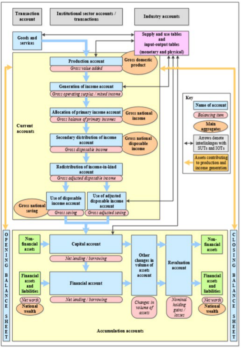
Handbook on Supply and Use Tables and Input-Output Tables with Extensions and Applications
9
Figure 1.1 Overview of the links between SUTs and the SNA framework
Compiled by Sanjiv Mahajan, May 2014
1.25. The first purpose of describing production, income, expenditure and financial flows, and
balance sheets, is served by grouping institutional units into institutional sectors on the basis of
Handbook on Supply and Use Tables and Input-Output Tables with Extensions and Applications
10
their principal functions, behaviour and objectives. The SNA enables a complete set of flow
accounts and balance sheets to be compiled for each sector and subsector, and also for the total
economy. The five institutional sectors distinguished in the SNA are the following:
• Non-financial corporations
• Financial corporations
• General government
• Households
• Non-profit institutions serving households
1.26. The SNA also describes the transactions between these five institutional sectors and the
rest of the world. These institutional sectors can be further split into subsectors, for example,
general government can be split into central government and local government.
1.27. The second purpose of describing processes of production and for input-output analysis is
served by the grouping of local kind-of-activity units (or establishments) into industries, on the
basis of their type of activity. An activity is characterized by an input of products, a production
process and an output of products.
1.28. In order to ensure consistency between SUTs and the institutional sector accounts, a link
table is compiled as an integrated part of the system. In this link table, a cross-classification of
output, intermediate consumption, components of value added (and other possible variables of
industries) between the industries and the institutional sectors is shown. Thus, this table links the
main macroeconomic variables from the SUTs to the institutional sector accounts, providing a
picture of local kind-of-activity units and one based on institutional units. As both types of units
are classified differently, the link table also provides a picture of the relations of output,
intermediate consumption, value added, and other variables, originating in the different industries
and institutional sectors.
1.29. The SUTs – consistent with the national accounts – are normally produced in connection
with the final or benchmarked versions of the macroeconomic data some two or three years after
first preliminary results of the national accounts are published. The SUTs, however, should play a
more vital role at the heart of national accounts in the production of preliminary annual or even
quarterly accounts. Once the SUTs compilation system is in place on an annual basis, the statistical
benefits are significant.
1.30. SUTs can play various roles in the national accounts. One, for example, is to update SUTs
– often in a more aggregated version – from the previous year with information available for the
preliminary estimates in order to have a complete set of SUTs available that are consistent with
the national accounts. This procedure is a good method for revealing inconsistencies in the
aggregated preliminary national accounts. Another role of SUTs could arise from new information

Handbook on Supply and Use Tables and Input-Output Tables with Extensions and Applications
11
in a situation in which new, and more, detailed information on total supply and exports is available
at an early stage, the structure and relationships in the SUTs of the previous year could be used to
project SUTs for domestic output and imports.
1.31. The compilation of SUTs was in the past associated solely with the construction of IOTs.
The SUTs were therefore seen as an intermediate step in the compilation of IOTs. This meant,
effectively, that the SUTs were only compiled out after the compilation of the national accounts
had been completed. This approach, in fact, has significant limitations because the independently
calculated national accounts aggregates had to be kept unchanged despite inconsistencies
identified through the SUTs system.
1.32. SUTs are now seen as more than just as a step in the construction of IOTs: it is the SUTs
that provide the ideal framework guaranteeing the coherency and consistency of supply and use of
products in the system in current prices, and in volume terms, thereby improving the quality of the
national accounts, and in turn the key economic aggregates.
1.33. The compilation of SUTs is thus recommended as part of the regular annual compilation
of national accounts. The annual compilation of SUTs is also one of the recommended data sets
used in assessing the scope of implementation of the 2008 SNA.
3
The compilation of SUTs on a
quarterly basis can also play a role in improving the quality and coherence of quarterly national
accounts (the role played by SUTs in quarterly national accounts is further elaborated in chapter
14).
1.34. The approach to the compilation of SUTs as an integral component of the production of
national accounts may be formulated in general terms as follows:
• SUTs are produced as a central element of the compilation of national accounts with a view
to providing a key link to various parts of the SNA framework.
• SUTs provide a statistical framework representing the most efficient means of incorporating
all basic data – aggregated or detailed – covering the components of the three approaches to
measuring GDP, and linking to the institutional sector accounts in a systematic way.
• SUTs effectively ensure the consistency and reconciliation of results at a detailed level and
thereby improve the overall quality of the national accounts.
• SUTs are compiled and balanced in both current prices and in volume terms.
• SUTs are produced annually or even, if possible, on a quarterly basis, the ideal option.
3
See table 2 of the 2011 report of the Intersecretariat Working Group on National Accounts to the United Nations
Statistical Commission at its forty-second session (E/CN.3/2011/6), available at:
http://unstats.un.org/unsd/statcom/doc11/2011-6-NationalAccounts-E.pdf.
Handbook on Supply and Use Tables and Input-Output Tables with Extensions and Applications
12
• SUTs can provide a powerful feedback mechanism on the coherency and consistency of
source data, such as business surveys, and on the classification of units on the business
register.
1.35. When balanced, SUTs provide a coherent, consistent and wholly integrated suite of
statistics for a single period (for example, a year), which include:
• A single estimate of GDP in current prices and in volume terms, which is underpinned with
components of the production, income (only in current prices) and expenditure approaches
to measuring GDP
• Detailed goods and services account in current prices and in volume terms (not by
institutional sector)
• Production accounts by industry and by institutional sector in current prices and in volume
terms.
• Generation of income accounts by industry and by institutional sector (both in current prices
only)
• Link to the use of disposable income account through the flows of final consumption
expenditures and capital account through gross capital formation (and its components)
balanced via SUTs.
1.36. These guidelines should form part of the strategic tools used to improve the quality of the
national accounts.
D. Objectives of this Handbook
1.37. The theoretical development of IOTs has a long history. Box 1.1 provides a description of
the evolution of both IOTs and SUTs within the context of national accounts. The United Nations
Statistics Division has followed the theoretical development and the practical work of national
statistics offices on IOTs and SUTs from the outset. Starting in 1996, it has prepared a number of
publications, under the guidance of the United Nations Statistical Commission, such as those listed
among the references under United Nations, 1966, 1973 and 1999, to share practices, update the
methodology in line with the updates of the SNA, and provide guidance on the compilation of
IOTs.
1.38. This Handbook continues those efforts in cooperation with other international
organizations and experts, providing practical and step-by-step guidance for the compilation of
SUTs and IOTs based on the latest international statistical standards set out in the 2008 SNA and
the sixth edition of the International Monetary Fund (IMF) Balance of Payments and International
Investment Position Manual (BPM 6) (IMF, 2009).

Handbook on Supply and Use Tables and Input-Output Tables with Extensions and Applications
13
Box 1.1 Evolution of the SUTs and IOTs within the national accounts
The national accounting system is continuously evolving across the various domains to reflect developments in
and improvements to the quality of economic statistics and the evolution of economies, with a view to providing
a relevant measurement of the economy. Over the past four centuries many significant contributions have been
provided by people from various disciplines and countries, resulting in the system as it stands today and how it
relates to SUTs and IOTs. Below is a short description of this evolution.
Wassily Leontief (1905–1999), who is often referred to as the pioneer of input-output-based economics, made
the first of many key contributions with the publication of his article “Quantitative input and output relations in
the economic system of the United States”. This article discussed the construction of an economic transactions
table that Leontief had based on the tableau économique, proposed by François Quesnay in 1758.
The framework was developed and applied as an economic tool with the construction of the first IOTs for the
United States covering the years 1919 and 1929 published in 1936. Later, Leontief developed the first input-
output-based model, which was based on theories developed by Leon Walras published in 1874 and 1877.
Leontief‘s pioneering work was recognized by the award to him of the Nobel Prize in Economics in 1973. As
a result, input-output analysis has become a major tool in developing quantitative economics as a science.
The role of SUTs and IOTs has evolved within national accounts. The 1953 SNA (United Nations, 1953)
included no reference to SUTs or IOTs. The 1968 SNA (United Nations, 1968), however, presented the
integration of an input-output framework into the integrated economic accounts of the SNA. The conceptual
development of the integrated economic accounts of the SNA earned Richard Stone the Nobel Prize in
Economic Science in 1984, for having made fundamental contributions to the development of the SNA and
having thereby greatly improved the basis for empirical economic analysis.
Alongside Leontief and Stone, other Noble laureates include Ragnar Frisch and Jan Tinbergen in 1969, Paul
Samuelson in 1970, Simon Kuznets in 1971, John Hicks in 1972 and James Meade in 1977, who have all
contributed to the foundations of the measurements used in today’s SNA and the interlinkages between various
sectors and activities in an economy.
The latest evolution of SUTs was recognized in the 1993 SNA (United Nations, CEC, IMF, OECD and World
Bank, 1993), chapter XV of which covered both SUTs and IOTs. With the latest version of the SNA, the 2008
SNA, the role and applications of SUTs have been further enhanced, and this in turn will help to meet many
analytical needs, as reflected in chapters 14 and 28 of the 2008 SNA.
1.39. This Handbook may, therefore, be viewed as an update of the United Nations Handbook
of Input-Output Table Compilation and Analysis (United Nations, 1999). In response, however, to
the ever-increasing importance of SUTs in their own right, this Handbook extends the scope of the
previous publication by providing a more detailed description and compilation guidance for SUTs.
As stated in the 2008 SNA, “only supply and use tables provide a sufficiently rigorous framework
to eliminate discrepancies in the measured flows of goods and services throughout the economy
to ensure the alternative measures of GDP converge to the same value” (2008 SNA, para. 14.15).
1.40. The Handbook builds on the experience, practices and guidance available at national and
regional level, such as the Eurostat Manual of Supply, Use and Input-Output Tables (Eurostat,
2008). At the same time, however, it provides an innovative approach to the compilations of SUTs
and IOTs in the following three main areas:
• Underlying use of an integrated approach to statistics

Handbook on Supply and Use Tables and Input-Output Tables with Extensions and Applications
14
• Use of a business model for the compilation of SUTs and IOTs linking the various parts
through an H-Approach compilation scheme
• Mainstreaming of environmental considerations, through the inclusion of the environmental
focus of chapter 13 at the core of part three of the Handbook
1.41. The compilation guidance provided in this Handbook relies on an integrated statistics
approach whereby the production of statistics in the various domains is not seen in isolation but as
part of an integrated process using common concepts, definitions, business registers and frames,
statistical units, estimation methods and data sources to improve the consistency of the statistics
compiled, to reduce the respondent burden, and potentially to reduce the statistical agency costs.
In particular, the consistency of the basic economic information that feeds into the national
accounts and the SUTs with the classifications, concepts and definitions of the 2008 SNA greatly
reduces the discrepancies across data from different sources, thus facilitating their reconciliation
as part of the integration process. The integrated statistics approach is described in the Guidelines
on Integrated Economic Statistics (United Nations, 2013).
1.42. This Handbook follows the Generic Statistical Business Process Model (GSBPM)
(UNECE, 2013) to describe the production of statistics in a general and process-oriented manner.
The underlying concepts and principles of the GSBPM have been followed in describing the
business process and stages of the statistical production processes underpinning the compilation
of SUTs and IOTs. Chapter 3 of this Handbook describes these links in more detail in the context
of SUTs and IOTs. In addition, the chapters in parts two and three of the Handbook are linked to
the different parts of these stages of the statistical production process.
1.43. With the adoption of the System of Environmental-Economic Accounting (SEEA) (United
Nations, European Commission, FAO, IMF, OECD and World Bank, 2014) by the United Nations
Statistical Commission, the extension of SUTs and IOTs to include environmental flows in
monetary and physical terms has become an internationally agreed standard. Including
environmental consideration from the outset in the compilation of SUTs brings a number of
advantages. It facilitates the integration and reconciliation of the information, it enhances the
quality of the information, and it significantly increases the uses to which the tabulations may be
put.
1.44. In line with the United Nations Statistical Commission,
4
this Handbook recommends the
annual compilation of SUTs. In addition, the Handbook promotes the compilation of these tables
as an integral part of the compilation of national accounts in order to ensure full consistency of the
basic data and also of the macroeconomic estimates that are derived from the accounts.
4
See the 2011 report of the Intersecretariat Working Group on National Accounts to the United Nations Statistical
Commission at its forty-second session (E/CN.3/2011/6), available online at:
http://unstats.un.org/unsd/statcom/doc11/2011-6-NationalAccounts-E.pdf
Handbook on Supply and Use Tables and Input-Output Tables with Extensions and Applications
15
1.45. The Handbook provides a consistent numerical example of SUTs and IOTs that runs
throughout the chapters (as far as practically possible), in order to facilitate understanding of the
various compilation steps. It also provides examples of best practices to illustrate certain aspects
of the compilation of SUTs. It should be noted that, in the numerical examples provided in the
Handbook, the numbers may not add up exactly to the totals because of rounding.
1.46. The target audience for this Handbook mainly includes compilers of SUTs and IOTs with
a basic knowledge and understanding of the SNA. Since, however, the Handbook provides an
overview of the whole statistical production process, managers or staff in charge of the programme
of national accounts and of economic and environmental accounts would also benefit from the
Handbook in gaining an overall understanding of the requirements for the compilation of SUTs
and IOTs. Lastly, analytical users may also benefit from perusing the Handbook, as it would
provide them with a better understanding of the compilation steps, thus increasing the analytical
applications of SUTs and IOTs.
E. Structure of the Handbook
1.47. The Handbook consists of the following four main parts:
• Part one, providing an introduction to the Handbook, set out in chapter 1.
• Part two, describing the overview of SUTs and IOTs, the fundamental building blocks
required, cross-cutting issues and the main stages of the GSBPM – namely, the design,
building and collection phases. Part two comprises chapters 2–4.
• Part three, describing the compilation, balancing and dissemination phases of SUTs and
IOTs. This also includes the physical SUTs (PSUTs), environmentally extended IOTs (EE-
IOTs) and the SUTs links to the quarterly national accounts. Part three comprises chapters
5–15.
• Part four, providing examples of the extensions and applications of SUTs and IOTs. Part
four comprises chapters 16–21.
Part one
1.48. As indicated above, chapter 1 provides an introduction to the Handbook; it describes the
importance of SUTs and IOTs for statistical purposes (for example, compilation of annual and
quarterly national accounts, etc.), for policymaking and for analytical purposes (for example,
economic forecasting, assessing the impact of globalization). It also provides a general description
of the SNA and where the SUTs fit within the SNA framework. This chapter also describes the
overall approach of the Handbook (including in comparison to previous handbooks) to the
compilation of SUTs and IOTs and provides a general outline of its contents.
Handbook on Supply and Use Tables and Input-Output Tables with Extensions and Applications
16
Part two
1.49. Chapter 2 provides a conceptual overview of SUTs and IOTs and describes the basic
elements determining their structure and compilation. These include the accounting principles of
the SNA, the classifications of economic activities and products, the choice of the statistical units
and how they affect SUTs and IOTs, and the valuation in SUTs and IOTs. The chapter identifies
the advantages of compiling SUTs as an integral part of the national accounts and how the SUTs
are used to obtain consistent estimates of GDP. It also describes in more detail the extended
perspective adopted in this Handbook to SUTs and IOTs, incorporating an environmental
dimension which makes possible an integrated overview of the framework from the very outset.
1.50. Chapter 3 provides an overview of the different phases that constitute the statistical
production process of SUTs and IOTs, based on the stages of the GSBPM and in line with the
United Nations Guidelines on Integrated Economic Statistics (United Nations, 2013). This chapter
also provides an overview of the different institutional set-ups in countries which may have an
impact on the compilation process. The compilation phases specific to SUTs and IOTs are
presented in this chapter together with a link to the relevant chapters of the Handbook.
1.51. Chapter 4 covers specific phases of the GSBPM, namely the specify needs, design, build
and collect phases. It provides a description of the elements that should be considered and carefully
evaluated at the beginning of the compilation process, such as the level of detail of the industry
and products in the tables, the compilation schedule, the revision policy, resources, typical data
sources, and others. These and other issues are covered in this chapter, thus providing a foundation
for the compilation of SUTs and IOTs.
Part three
1.52. Chapter 5 describes the conceptual and practical aspects of the compilation of the supply
table and how the so-called “unbalanced” supply table is put together from the typical data sources
for SUTs, such as business surveys, administrative data and others.
1.53. Chapter 6 describes the conceptual and practical aspects of the compilation of the use table.
As in chapter 5, this chapter shows how an unbalanced use table is constructed on the basis of
typical data sources.
1.54. Chapter 7 describes how to compile the valuation matrices necessary to bridge the different
valuation concepts of the product flows. This chapter covers the main concepts and methodologies
of compiling matrices for trade margins, transport margins, taxes on products and subsidies on
products.
1.55. Chapter 8 describes the structure of the imports use table and the domestic use table and
the steps necessary to disaggregate the use table into an imports use table and a domestic use table.
Historically, the compilation of these tables was largely viewed as an intermediate – though not
Handbook on Supply and Use Tables and Input-Output Tables with Extensions and Applications
17
essential – step in the compilation of IOTs. That said, however, the imports use table and the
domestic use table are becoming increasingly important in their own right for analytical purposes.
1.56. Chapter 9 covers the compilation of SUTs in volume terms. It follows the recommendation
that SUTs should simultaneously be compiled in current prices and in volume terms. The
compilation of SUTs in volume terms can start after the SUTs have been compiled in current prices
(although the current price tables do not need to be balanced) but there is need for a simultaneous
presentation of volume and price indices.
1.57. Chapter 10 describes the importance of linking SUTs and the institutional sector accounts,
which involve data by industry that are to be subdivided according to the institutional sectors to
which the units within each industry are assigned. The chapter provides guidance on how to
compile the cross-tabulation between industries and institutional sectors and presents various
approaches that may be followed in establishing the link between the SUTs and the institutional
accounts. It also identified certain issues that may arise in the compilation of the linking table.
1.58. Chapter 11 describes the manual and automated balancing procedures of SUTs in both
current prices and in volume terms. This is important for full consistency of the detailed
information. The various checks related to product, industry and macro identities, benchmarking
with national accounts, and comparison with previous SUTs, if available, are explained. It is
recommended that SUTs should be produced and balanced simultaneously at basic and purchasers’
prices and also for domestic and imported products, all of which should be both in current prices
and in volume terms. A further dimension, and challenge to be surmounted, is the need to cover
both annual SUTs and, if possible, quarterly SUTs.
1.59. The sequence of chapters represents the preferred scenario for the compilation of SUTs.
Different approaches may be followed, however. An increasing number of countries have achieved
the preferred scenario. This scenario for the compilation of SUTs and IOTs may be seen as
ambitious but it can be realized through gradual improvements in source data, production
processes and the information technology environment.
1.60. Chapter 12 provides an overview of the IOTs (product by product and industry by industry)
and describes the methods and the underlying assumptions for transforming SUTs into IOTs. The
compilation of IOTs is quite different in nature from that of SUTs and relies on the availability of
SUTs. The compilation of IOTs is considered more as an analytical step than a compilation process
and, for this purpose, is viewed as a transition from statistics to modelling.
1.61. Chapter 13 describes the structure of the SUTs in physical units where additional rows and
columns are added to show flows from the environment to the economy and vice versa. This
chapter also describes typical data sources for the compilation of these tables and examples of
specific issues in which the SEEA and the SNA differ (for example, the treatment of international
flows and the treatment of goods for processing), and shows how standard economic IOTs in
monetary units may be extended to include information on the environment in physical units in
Handbook on Supply and Use Tables and Input-Output Tables with Extensions and Applications
18
the environmentally extended IOTs. Physical IOTs are also an extension of the SUTs framework,
extended to take into account environmental considerations. They consist of a transformation of
the PSUTs. Given certain conceptual and practical issues in the compilation of physical IOTs,
however, the focus of the 2012 SEEA – and thus of this chapter – has shifted towards the
compilation of environmentally extended IOTs rather than physical IOTs. Examples of two
country practices are also presented in this chapter.
1.62. Chapter 14 provides an overview of how SUTs may be used to improve the quarterly
national accounts. Since there are various scenarios that can be used in practice, this chapter
focuses only on three main situations which illustrate the use of SUTs to various degrees in the
compilation of the quarterly national accounts.
1.63. Data dissemination is an important activity for any statistical production process, as it
provides users with a range of statistics produced to internationally agreed guidelines. Presenting
SUTs and IOTs to users in a clear, transparent and user-friendly manner is thus an important task
for the statisticians. Chapter 15 provides an overview of the elements that should be considered
when disseminating SUTs and IOTs, such as the identification of users’ needs in order to tailor
dissemination to the main types of users of SUTs and IOTs, the importance of having a
dissemination strategy and the elements that should be covered in the strategy. Reference to the
Statistical Data and Metadata Exchange (SDMX) for SUTs and IOTs is also provided in this
chapter.
Part four
1.64. Chapter 16 describes the methods for compiling regional (subnational) SUTs and the main
compilation issues, such as the disaggregation of the information at subnational level, among
others. Different issues and challenges are covered through a bottom-up and top-down compilation
approach.
1.65. Although the focus of this Handbook is mainly on the compilation of national SUTs and
national IOTs, there is a growing demand for these instruments to capture the structure and
mechanism of the cross-border fragmentation of production activities. Chapter 17 provides an
overview of multi-country SUTs and IOTs, the main compilation issues, and a simplified
compilation procedure. This chapter also reviews current international initiatives in this area.
1.66. Chapter 18 deals with the projections of SUTs and IOTs. Many users also require
comparable input-output products that are comparable in terms of frequencies and timeliness. For
example, some countries produce quarterly SUTs, some countries produce annual SUTs and some
countries produce SUTs on a less regular basis. Consequently, a variety of methods, techniques
and approaches exist for the projection of SUTs and IOTs and for dealing with data gaps. These
techniques also can help producers, for example, to deal with periods between benchmarked years.
This chapter examines various methods and techniques used, along with a range of literature
available on how to surmount the problem of incomplete data, thus allowing the estimation and
Handbook on Supply and Use Tables and Input-Output Tables with Extensions and Applications
19
projection of IOTs. The chapter also presents a numerical example for three methods: the
generalized RAS, the SUT-RAS and the Euro methods.
1.67. Chapter 19 describes the main extensions of supply, use and input-output tables as part of
a satellite system which is routinely used for economic analysis. Several examples of the
disaggregation of the use table and various satellite accounts are reviewed, including such
extensions as social accounting matrices, extended IOTs and other satellite systems.
1.68. Chapter 20 describes the different types of input-output models and provides a broad
overview illustrating the benefits and the approaches used. The traditional quantity model and
price model of input-output analysis are presented for monetary IOTs and physical IOTs. Input
and output coefficients, the Leontief inverse, price and quantity models, indicators, multipliers and
inter-industrial linkages were developed for an empirical extended IOT, with extensions for gross
fixed capital formation, capital stock, employment, energy, air emissions, waste, sewage and
water.
1.69. Chapter 21 provides examples of compilation practices from various countries with
different statistical systems. In general, the compilation practices can vary greatly depending on
the resources available, the statistical infrastructure, registers, surveys, methodologies and other
factors. This chapter provides guidance for countries with limited statistical resources and
illustrates differences and challenges in the compilation of SUTs and IOTs.
Handbook on Supply and Use Tables and Input-Output Tables with Extensions and Applications
21
Part two
Handbook on Supply and Use Tables and Input-Output Tables with Extensions and Applications
23
Chapter 2. Overview of the supply and use tables and input-output tables
A. Introduction
2.1. Before providing step-by-step guidance on the compilation of SUTs and IOTs, it is
important to ensure a general understanding of the two sets of tables. The main objective of this
chapter is, therefore, to provide an overview of SUTs and IOTs, which may be found in sections
B and C, respectively. Section D introduces the fundamental elements of the SUTs and IOTs, such
as the underlying classifications, the statistical units and the valuation methods. Some of these
elements are discussed in more detail in subsequent chapters. Lastly, section E elaborates on the
importance of compiling SUTs as an integral part of the national accounts.
2.2. Although this chapter covers a wide range of challenges and issues that must be tackled
when planning and building a new system of SUTs and IOTs, all aspects may not be achievable in
countries with limited resources. It is worth recognizing that a system may be established with a
moderate level of ambition using available data, even if these are incomplete. Nonetheless, it is
preferable to have a SUTs-type environment for reconciliation of the various statistical sources,
rather than only an unbalanced series of national accounts aggregates.
B. Overview of SUTs
2.3. The SUTs describe the whole economy by industry (for example, the motor vehicle
industry) and by product (for example, sports goods). The tables show links between components
of GVA, industry inputs and outputs, and product supply and use. The SUTs link different
institutional sectors of the economy (for example, non-financial corporations) together with details
of imports and exports of goods and services, final consumption expenditure of government,
household and non-profit institutions serving households (referred to as NPISHs), and capital
formation.
2.4. As their name suggests, SUTs consist of two interlinked tables: the supply table and the
use table. The supply table shows the supply of goods and services by type of product and by type
of industry, distinguishing between supply by domestic industries and imports of goods and
services. In other words, the supply table provides information on the output (by product)
generated by economic activities and the imports (by product) from abroad. The totals in the last
column represent the total supply by products and the totals in the bottom row represent the total
output by economic activity and total imports. A simplified supply table is presented in Table 2.1
below.

Handbook on Supply and Use Tables and Input-Output Tables with Extensions and Applications
24
Table 2.1: Simplified structure of the supply table
2.5. The second table is the use table, which provides information on the uses of the different
products. The use table shows the use of goods and services by type of product and by type of use,
in other words, as intermediate consumption by industry, final consumption, gross capital
formation or exports. Furthermore, the table shows the components of gross value added by
industry – namely, compensation of employees, other taxes less subsidies on production,
consumption of fixed capital and net operating surplus. While the totals by row represent the total
uses by product, the total by column represent the total output by economic activity, total final
consumption, total gross fixed capital formation and total exports. Table 2.2 below shows the
simplified structure of the use table.
Table 2.2: Simplified structure of the use table
2.6. The classification of products, in practice, is often more detailed than the classification of
industries, thus generating rectangular SUTs. For example, the output of the dairy industry is
separately shown in the SUTs for the products of processed milk, butter, yoghurt, cheese and so
forth, and not as only one aggregate product for all dairy products.
2.7. There are three basic identities that hold between the supply table and the use table. The
first identity corresponds to the fundamental identity in national accounts, whereby for each
economic activity the following holds:
Identity (1) Output = Intermediate consumption + GVA
Agriculture,
forestry, etc.
Mining and
quarrying
… Services
Agriculture, forestry, etc.
Ores and minerals, etc.
…
Services
Total
Total imports Total supply
Total output by industry
Industries
Products
Industries
Imports
Total
Output by product by industry
Imports by
product
Total supply
by product
Agriculture,
forestry, etc.
Mining and
quarrying
… Services
Final
consumption
Gross capital
formation
Exports
Agriculture, forestry, etc.
Ores and minerals, etc.
…
Services
Value added
Value added
Total
Empty cells by definition
Total
Intermediate consumption by product and by industry
Final uses by product and by category
Total use by
product
Value added by component and by industry
Total output by industry
Total final uses by category
Industries
Products
Industries
Final uses

Handbook on Supply and Use Tables and Input-Output Tables with Extensions and Applications
25
2.8. The second identity is that the total supply by product is equal to the total use by product.
This means that the amount of products available for use in an economy must have been supplied
either by domestic production or by imports, and the same amount of products entering an
economy in an accounting period must be used for intermediate consumption, final consumption,
capital formation or exports. This means that, for each product (or group of products):
Identity (2) Output + Imports = Intermediate consumption + Final consumption +
Capital formation + Exports
2.9. Another important identity which is also key when linking the production and income
approaches to calculating GDP and the industry and institutional sector dimension through the
SUTs is the following:
Identity (3) For each industry, the GVA using the production approach equals the
GVA estimate using the income approach.
2.10. These identities are fundamental in the balancing process that is carried out when
compiling SUTs both in current prices and in volume terms, all through a time series dimension.
2.11. Once balanced, the supply table and the use table can be integrated into a single matrix –
often referred to as the SUTs framework, which is shown in Table 2.3 below. This table clearly
shows the two basic identities linking the SUTs. The total supply by product (left part of the bottom
row of Table 2.3) equals the total use by product (top part of the last column of Table 2.3) and the
total outputs by industry are identical in both SUTs (the middle part of the bottom row equals the
middle part of the last column). The schematic view of SUTs in Table 2.3 also serves as the
underlying matrix for projection methods (see chapter 18).
Table 2.3: Supply and use tables framework
2.12. SUTs thus bring together the components of each of the three approaches to measuring
GDP– namely, the production, income and expenditure approaches:
(a) Production approach:
Agriculture,
forestry, etc.
Ores and
minerals, etc.
… Services
Agriculture,
forestry, etc.
Mining and
quarrying
… Services
Final
consumption
Gross capital
formation
Exports
Agriculture, forestry, etc.
Ores and minerals, etc.
…
Services
Agriculture, forestry, etc.
Mining and quarrying
…
Services
Value added
Value added
Imports
Total
imports
Total
Empty cells by definition
Total output
by industry
Value added by component and by industry
Total imports by product
Total
Products
Intermediate consumption by product and by
industry
Final uses by product and by category
Total use by
product
Products
Industries
Final uses
Total supply by product
Total output by industry
Total final uses by category
Industries
Output by product by industry
Handbook on Supply and Use Tables and Input-Output Tables with Extensions and Applications
26
GDP = Output (at basic prices) - Intermediate consumption + Taxes less subsidies
on products
(b) Income approach:
GDP = Compensation of employees + Gross operating surplus + Other taxes less
subsidies on production + Taxes less subsidies on products
(c) Expenditure approach:
GDP = Final consumption + Gross capital formation + Exports - Imports
2.13. When balanced, SUTs show, by definition, a single estimate of GDP both in current prices
and in volume terms. This underlines the importance of the recommendation that SUTs be
compiled as part of the annual regular compilation of the national accounts, as they ensure the
consistency and coherence of the national accounts components, namely, goods and services
account, production account (by industry and by institutional sector) and generation of income
account (by industry and by institutional sector), and make it possible to derive a single estimate
of GDP. The institutional sector links are covered in more detail in chapter 10.
2.14. The SUTs also have links to other accounts, such as disposable income accounts (covering
variables like household final consumption expenditure) and accumulation accounts (covering
variables like gross fixed capital formation as part of the capital account).
2.15. Producing annual SUTs simultaneously both in current prices and in volume terms
(preferably, when two successive years of current price SUTs are available) ensures coherence and
consistency for both price and volume measures. In addition, this approach allows for the
estimation of the volume of GVA through what may be termed “double deflation”, where GVA is
derived by deducting intermediate consumption in volume terms from total output in volume
terms. This can be achieved on the basis of an individual unit, industry, institutional sector, and
for the whole economy.
2.16. SUTs can also be compiled on a quarterly basis to derive official estimates of quarterly
GDP. Developing quarterly SUTs may be highly demanding in terms of resources, time and data
availability but have the advantage of significantly improving the quality of the estimate of
quarterly GDP.
2.17. Figure 2.1 provides a graphical overview of the SUTs, explicitly identifying the main
identities that are ensured in balanced SUTs. Box 2.1 presents a numerical example of balanced
SUTs.
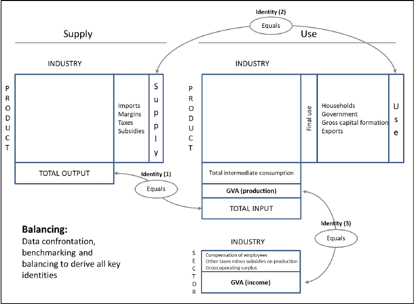
Handbook on Supply and Use Tables and Input-Output Tables with Extensions and Applications
27
Figure 2.1: Graphical overview of supply and use tables
2.18. The use table records the intermediate consumption and final uses by type of product but
it does not distinguish between the consumption of domestically produced goods and services and
that of imported goods and services. Although such a split is not a necessary condition for the
creation of balanced SUTs in current prices, it is a key step linking SUTs and IOTs. The
disaggregation of the use table into two tables, the domestic use table and the imports use table, is
shown in Box 2.2, with a numerical example.
2.19. The compilation of the imports use table is necessary to ensure good quality volume
estimates (in particular, GVA by industry) and these tables are becoming increasingly important
owing to the growing impact of globalization and the need to measure global value chains and
trade in value added.

Handbook on Supply and Use Tables and Input-Output Tables with Extensions and Applications
28
Box 2.1 Numerical example of the SUTs system
The supply table shows the supply of goods and services by product and by type of supplier, distinguishing supply
by domestic industries and imports of goods and services. The domestic output of industries is shown by products.
The vector of imports comprises the nation’s total imports of goods and services by product.
The use table shows the use of goods and services by product and by type of use, i.e. as intermediate consumption
by industry, final consumption expenditure, gross capital formation and exports of goods and services. The
intermediate uses and final uses reflect the consumption of domestically produced goods and services and also of
imported goods and services. Furthermore, although the table is shown in summary form, it should be noted that
there are components underlying the headings, for example, GVA can be split between compensation of employees,
other taxes less subsidies on production, consumption of fixed capital and net operating surplus.
Note that, for illustrative purposes, it is assumed that the SUTs presented here are compiled on a consistent valuation
basis.
2.20. Once the imports use table is constructed, the domestic use table can be estimated by
subtracting the imports use table from the use table. The imports use table and the domestic use
table form the basis for the construction of input imports tables and domestic IOTs, respectively.
More detail may be found in chapters 8 and 12.
Supply table
Agriculture
Manufacturing
and
construction
Services
Agriculture
270 30 50 20 370
Manufacturing
6 380 87 42 515
Construction
4 50 13 8 75
Trade, transport and communication
10 15 210 7 242
Finance and business services
6 17 240 11 274
Other services
4 8 100 12 124
Total
300 500 700 100 1 600
Use table
Agriculture
Manufacturing
and
construction
Services
Final
consumption
expenditure
Gross capital
formation
Exports
Agriculture
34 59 93 131 21 32 370
Manufacturing
97 107 57 122 73 59 515
Construction
9 12 4 17 30 3 75
Trade, transport and communication
42 24 11 140 20 5 242
Finance and business services
14 53 42 116 31 18 274
Other services
14 35 22 35 10 8 124
Taxes less subsidies on products
4 5 12 52 6 1 80
GVA
86 205 459 750
Total 300 500 700 613 191 126 2 430
Supply and use tables framework
Agriculture Manufacturing Construction
Trade, transport
and
communication
Finance and
business
services
Other
services
Agriculture
Manufacturing
and
construction
Services
Final
consumption
expenditure
Gross
capital
formation
Exports
Agriculture
34 59 93 131 21 32 370
Manufacturing
97 107 57 122 73 59 515
Construction
9 12 4 17 30 3 75
Trade, transport and communication
42 24 11 140 20 5 242
Finance and business services
14 53 42 116 31 18 274
Other services
14 35 22 35 10 8 124
Agriculture
270 6 4 10 6 4 300
Manufacturing and construction
30 380 50 15 17 8 500
Services
50 87 13 210 240 100 700
Taxes less subsidies on products
4 5 12 52 6 1 80
GVA
86 205 459 750
Imports
20 42 8 7 11 12 100
Total 370 515 75 242 274 124 300 500 700 613 191 126 4 030
= Zero by definition
Final use
Total
Total use
Industries
Industries
Imports
Total supply
Products
Industries
Products
Products
Products
Industries
Final use

Handbook on Supply and Use Tables and Input-Output Tables with Extensions and Applications
29
Box 2.2 Numerical example showing a use table split between consumption of domestic
production and imports
The domestic use table is derived by subtracting the imports use table from the total use table shown in box 2.1.
The imports of goods and services are then shown separately as a new row denoted as “Imports” in the domestic
use table. The domestic use table shows the input requirements of industries in terms of domestic intermediates,
imported intermediates and primary inputs (GVA). It also shows the use of domestic output of products for
intermediate uses and final uses.
The imports use table includes information on the use of imported products for intermediate consumption and
final uses and the column totals, which match the estimates shown in the “Imports” row.
1. Supply and use tables in current prices and in volume terms: H-Approach
2.21. The SUTs framework not only constrains the current value estimates of supply and use of
products to balance exactly, it also provides a means of ensuring that the corresponding volume
estimates in previous years’ prices are balanced and that the series of prices implied by the
existence of one table in current prices and one in volume terms are strictly consistent. In general,
the best way to ensure mutual consistency is to prepare the SUTs in current values and in volume
terms at the same time (2008 SNA, para. 14.136).
2.22. The compilation and balancing of SUTs in current prices and in volume terms for a
sequence of years also helps to balance the changes in volumes, values and prices in the best
possible way (the key condition for the attainment of this outcome is that SUTs are available in
current prices both for the current year and for the previous year). This approach ensures a high
degree of quality in terms of coherence and consistency over time – and recommended as the best
Supply table
Agricul-
ture
Manufact.
and
construction
Services
Agriculture
270
30
50
350
20 370
Manufacturing
6 380 87 473 42 515
Construction
4 50 13 67 8 75
Trade, transport and communication
10
15
210
235
7
242
Finance and business services
6 17 240 263 11 274
Other services
4 8 100 112 12 124
300 500 700 1 500 100 1 600
Use table Domestic use table
Agricul-
ture
Manufact.
and
construction
Services
Final
consumption
expenditure
Gross
capital
formation
Exports
Agricul-
ture
Manufact. and
construction
Services
Final
consumption
expenditure
Gross
capital
formation
Exports
Agriculture
34 59
93
131 21 32 370
Agriculture
30 50 90 130 20 30 350
Manufacturing
97 107 57 122 73 59 515
Manufacturing
85 90 51 120 70 57 473
Construction
9 12 4 17 30 3 75
Construction
5 10 3 16 30 3 67
Trade, transport and communication
42 24
11
140
20
5 242
Trade, transport and communication
40
20
10
140
20
5 235
Finance and business services
14 53 42 116 31 18 274
Finance and business services
10 50 40 115 30 18 263
Other services
14 35 22 35 10 8 124
Other services
10 30 20 35 10 7 112
Taxes less
subsidies on products
4
5 12 52 6 1 80
Imports
30 40 15 5 5 5 100
GVA
86 205 459
750
Taxes
less subsidies on products
4
5
12 52 6 1 80
Total 300 500
700 613 191 126 2 430
GVA
86 205 459 750
Output
300 500 700 613 191 126 2 430
Imports use table
Agricul-
ture
Manufact. and
construction
Services
Final
consumption
expenditure
Gross
capital
formation
Exports
Agriculture
4
9
3
1
1 2 20
Manufacturing
12 17 6 2 3 2 42
Construction
4 2 1 1 8
Trade, transport and communication
2
4
1 7
Finance and business services
4 3 2 1 1 11
Other services
4 5 2 1 12
Total 30 40 15 5 5 5 100
Empty cells by definition
Products
Total
Final use
Total use
Industries
Output
Imports
Total
supply
Products
Industries
Final use
Total
use
Industries
Products
Products
Industries
Final use
Total

Handbook on Supply and Use Tables and Input-Output Tables with Extensions and Applications
30
approach for the production of SUTs. Producing annual SUTs simultaneously both in current
prices and in volume terms also allows estimation of the volume of GVA through double deflation,
whereby GVA in previous years’ prices is derived by deducting intermediate consumption in
previous years’ prices from total output in previous years’ prices. Then, the change in volume of
GVA between each pair of consecutive years is given by the change of GVA in previous years’
prices compared to GVA of the previous year at current prices of that year.
2.23. The SUTs at purchasers’ prices and at basic prices in current prices and in volume terms
can be compiled and balanced sequentially or simultaneously. In both cases, powerful feedback
loops covering quality in terms of consistency and coherence are available. More details are
provided in chapters 9 and 11.
2.24. Figure 2.2 shows an overview of the H-Approach for an integrated compilation of SUTs
(and IOTs) in current prices and volume terms. The H-Approach is the recommended compilation
approach, which brings together the compilation of SUTs in current prices and volume terms, the
valuation at basic prices, producers’ prices and purchasers’ prices, and the links with the
compilation of IOTs. The matrices covering other taxes on production, other subsidies on
production, trade margins and transport margins are the valuation matrices which link between
basic prices, producers’ prices and purchasers’ prices.
Figure 2.2 Schematic overview of the compilation of SUTs and IOTs: H-Approach
Volume terms
SUTs
at purchasers’ prices
IOTs
Assumption applied
SUTs
at basic prices
Current prices
SUTs
at purchasers’ prices
IOTs
Assumption applied
SUTs
at basic prices
- Valuation matrices
- Split domestic use table
and import use table
Deflation
processes
- Valuation matrices
- Split domestic use table
and import use table
Handbook on Supply and Use Tables and Input-Output Tables with Extensions and Applications
31
2.25. The diagram in Figure 2.2 may be visualized as the letter “H” with the left vertical arm
representing SUTs and IOTs in current prices and the right vertical arm representing the SUTs and
IOTs in previous years’ prices. The horizontal transition represents the deflation process using, for
example, a combination of prices, volume indicators and rates of the previous year applied to the
volumes.
2.26. The SUTs in current prices are decomposed into the component parts (imports and the
valuation matrices on the left-hand side of the H-Approach), each of which is deflated separately
as appropriate (the join in the middle), and then added back to get to a purchasers’ prices valuation
in previous years’ prices (the right-hand side). This means that basic prices play the dominant role
in the process, and the initial compilation flow is from top left to middle left and that of deflation
to middle right, and then to top right.
2.27. When final use deflators are deemed to be better for final use components at purchasers’
prices, then the H-Approach allows for the use of higher quality deflators, which are perhaps more
appropriate. In these types of examples, it is possible to work with purchasers’ prices where the
data are believed to be more reliable, making appropriate adjustments, working from top right to
middle right, then onto middle left and to top left, and still ensuring a balance at each stage.
Similarly, if high quality volume indicators are available, then this can better inform, for example,
the step between the middle left and middle right with adjustments as appropriate.
2.28. For balancing purposes, areas such as value added tax (VAT) on products and changes in
inventories may be separated out as balanced matrices (whereby the impact on production, income
and expenditure is equal and the matrices are in balance) to avoid any balancing adjustments, but
this may overcomplicate the system.
2.29. It is important to note that the scheme presented in Figure 2.2 should not be taken as one
to be implemented as a whole. In practice, for example, if a country wants to focus exclusively on
the compilation of annual SUTs, the focus should be on the compilation steps of the SUTs within
the bold line box in Figure 2.2 which are recommended in order to achieve balanced SUTs in
current and in volume terms. If, however, a country wants to compile SUTs and IOTs, all the steps
in Figure 2.2 should be completed in order to guarantee important feedback loops and enhance the
quality of the tabulations.
2.30. When planning for the compilation of SUTs, it is useful to keep in mind the compilation
approach in Figure 2.2, since it is naturally linked to the production of time series of SUTs (and
IOTs) both in current prices and in previous years’ prices using chain-linked volumes. More detail
of this may be found in chapter 9. Although SUTs in volume terms for one period can be compiled
using SUTs in current prices for one period and deflators, the preferred approach contains a time-
series dimension and the following principles:
• To compile SUTs in volume terms, the following are needed:
Handbook on Supply and Use Tables and Input-Output Tables with Extensions and Applications
32
Balanced set of SUTs at purchasers’ prices in current prices for the present year and
the previous year
Deflators for each flow
• Previous year’s SUTs in current prices of that year are needed to derive volume estimates.
The SUTs in figure 2.2 are balanced for illustrative purposes. In reality, however, they may
be unbalanced and an iterative balancing process may be necessary. This allows for the first
SUTs in previous years’ prices to be compiled.
• Each transition stage is created in a balanced format which provides a much easier systematic
process and build. This means that each of the transition matrices covering taxes, subsidies,
trade and transport margins and import of goods and services will be balanced, in other
words, the supply-side row total will equal the use-side row total.
• For some of the variables, like household final consumption expenditure, there are already
present deflation approaches using consumer price indices to generate the corresponding
estimates in previous years’ prices. These estimates are likely to differ from those generated
with the H-Approach but would also feature in the reconciliation and balancing process of
the estimates, and form an example of working from right to left through balanced
adjustments.
2.31. The H-Approach provides a transparent, coherent and consistent approach for the
compilation and balancing of SUTs. For example, balancing adjustments to one part of the SUTs
can be assessed in terms of their impact on other areas of the SUTs, and also in terms of time
series.
2. PSUTs
2.32. The SUTs described in the previous sections are part of the 2008 SNA framework. As such,
they reflect the production boundary of the SNA and they are compiled in monetary units. The
tables can, however, be extended to include the environment as providers of natural inputs into the
economy and as absorbers of residuals from the economy. The extension of these tables and, more
generally, of the accounting framework of the SNA to include environmental considerations is
carried out in the 2012 SEEA. The SEEA enables the analyses of the interaction between the
environment and the economy, such as an assessment of the use of natural resources, the generation
of waste by the economy and waste flows into the environment.
2.33. The SEEA central framework comprises a sequence of accounts – namely, the SUTs in
monetary and physical units, the asset accounts in physical and monetary units, and environmental
activity accounts and related flows. The present Handbook covers the SUTs of the SEEA and, in
particular, since the monetary SUTs of the SEEA are the same as the SNA, the Handbook focuses
on the PSUTs of the SEEA. For additional information on the complete set of accounts of the
Handbook on Supply and Use Tables and Input-Output Tables with Extensions and Applications
33
SEEA, the reader is directed to the publication United Nations, European Commission, FAO, IMF,
OECD and World Bank (2014).
2.34. PSUTs are used to assess how an economy supplies and uses energy, water, materials, and
also their changes in production and consumption patterns over time, and therefore, in combination
with data from monetary SUTs, changes in productivity and intensity in the use of natural inputs
and the release of residuals can be examined. The structure of PSUTs is based on the monetary
SUTs with extensions to incorporate a column for the environment and rows for natural inputs and
residuals.
2.35. Table 2.4 and Table 2.5 provide the simplified structure of the physical supply table and
use table, respectively. In order to address specific environmental domains (for example,
accounting for water, energy, timber and other resources), these tables are compiled for a
disaggregation of products and industries which is relevant for the particular environmental
domain of interest. In the case of energy, for example, the products of interest that can be explicitly
shown in the table include coal, peat and peat products, natural gas and others. The industries of
interest include the main suppliers of energy products (for example, electricity generation,
manufacture of gas and other products) and the main users of energy products (for example,
manufacturing, transportation and others). These tables are compiled in monetary units – within
the SNA context – and in physical units as shown in Table 2.4 and Table 2.5.
2.36. In the PSUTs, the SUTs of the SNA are augmented to include a block of rows for “natural
inputs” and a block of rows for “residuals”. The block for natural inputs is used to describe the
flows from the environment to the economy; in other words, this block describes the extraction of
natural inputs (for example, water, energy resources and others) from their location in the
environment as a part of economic production processes or that are directly used in production.
Natural inputs may be, first, natural resource inputs, such as mineral and energy resources or timber
resources; second, inputs from renewable energy sources, such as solar energy captured by
economic units; or, third, other natural inputs such as inputs from soil (for example, soil nutrients)
and inputs from air (for example, oxygen absorbed in combustion processes) (2012 SEEA, para.
2.89). When an industry, for example, extracts water as part of the economic production process,
this is recorded in the block of natural inputs in the use table in Table 2.5. It is assumed that the
environment provides (that is, supplies) all the natural inputs that are used into the economic
production process.
2.37. The blocks for “residuals” represent the flows of solid, liquid and gaseous materials, and
energy, that are discarded, discharged or emitted to the environment (for example, emission to air)
by establishments and households through processes of production, consumption or accumulation
but that may also flow within the economy, as is the case when, for example, solid waste is
collected as part of a waste collection scheme (2012 SEEA, para. 2.92).

Handbook on Supply and Use Tables and Input-Output Tables with Extensions and Applications
34
2.38. The block for residuals in the supply table (Table 2.4) represents the flows of waste from
the economy to the environment and thus it includes the generation and disposal of waste during
economic production activities (generation of waste by industries) and generated during final
consumption (mainly by households). While the block of residuals in the use table (Table 2.5)
shows, for example, the collection and treatment of waste and other residuals by economic
activities, the accumulation of waste in controlled landfills and the residuals flows direct to the
environment.
Table 2.4 Schematic view of the physical supply table
Table 2.5 Schematic view of the physical use table
2.39. The supply and use identity applies to both physical and monetary flows. For each product
measured in physical terms (for example, cubic metres of timber), the quantity of output and
imports (total supply of products) must equal the quantity of intermediate consumption, household
final consumption, gross capital formation and exports (total use of products). The equality
between supply and use also applies to the total supply and use of natural inputs and the total
supply and use of residuals. In addition to the supply and use identity, the PSUTs incorporate the
Agriculture,
forestry, etc.
Mining and
quarrying
… Services
Mineral and energy resource
Water
…
Agriculture, forestry, etc.
Ores and minerals; etc.
…
Services
Solid waste
Wastewater
…
Empty cells by definition
C ells may contain relevant flows
Total supply
by residuals
Residuals
Residuals generated by industry
Residuals
generated
by final
consumtpion
Residuals from
scrapping and
demolition of
produced assets
Products
Output by product by industry
Imports by
product
Total supply
by product
Total
Natural
inputs
Flows from
the
environment
Total supply
by natural
inputs
Industries
Industries
Imports
Final
consumtpion
Gross capital
formation/
Accumulation
Environment
Agriculture,
forestry, etc.
Mining and
quarrying
… Services
Mineral and energy resource
Water
…
Agriculture, forestry, etc.
Ores and minerals; etc.
…
Services
Solid waste
Wastewater
…
Empty cells by definition
C ells may contain relevant flows
Residuals
C ollection and treatment of waste and other
residuals
Accumulation of
waste in
controlled
landfilled
Intermediate consumption by product and by
industry
Final uses by product and by category
Total use by
product
Total use by
residuals
Residual
flows direct
to the
enviornment
Total
Natural
inputs
Extraction of Natural inputs
Total use by
natural
inputs
Industries
Industries
Exports
Final
consumtpion
Gross capital
formation/Accu
mulation
Environment
Products
Handbook on Supply and Use Tables and Input-Output Tables with Extensions and Applications
35
input-output identity, implying that the total flows into the economy either are returned to the
environment or accumulate in the economy.
C. Overview of IOTs
2.40. For many analytical purposes, a transformation from a pair of SUTs into a single IOT where
total input (row totals) and total output (column totals) are equal brings considerable advantages.
IOTs have algebraic properties that make them particularly suitable for analyses that enable
estimates of the effects of changing relative prices, labour and capital requirements in the face of
changing output levels, the consequences of changing patterns of demand and so on. They may
also be used as the basis for an expanded version that may be used to estimate the demands made
by the economy on the environment (2008 SNA, para. 28.35).
2.41. An IOT is essentially derived from the use table, where either the columns representing
industries are replaced by products or where the rows representing the products are replaced by
industries through a transformation process which involves a range of assumptions. The resulting
intermediate consumption matrix is then square, showing products in both rows and columns or
industries in both. In both cases, the row totals for the complete matrix match the column totals
for the complete matrix, product-by-product matrix or industry-by-industry matrix as the case may
be (2008 SNA, para. 28.32). Of course, the classifications in the IOTs coincide with those in the
SUTs, as the former is a transformation of the latter.
2.42. It is recommended that the IOTs be derived from SUTs. The IOTs derived from the SUTs
further describe the interrelationships between industries and products, along with the sale and
purchase relationships between producers and consumers within an economy. They can be
produced to illustrate flows between the sales and purchases (final and intermediate) of industry
outputs (referred to as industry-by-industry tables) or to illustrate the sales and purchases (final
and intermediate) of product outputs (referred to as product-by-product tables).
2.43. The derivation of IOTs from the system of SUTs may also reveal inconsistencies and
weaknesses in the SUTs. This is made possible by the powerful quality-related feedback loop from
the IOTs to the SUTs and vice versa.
2.44. Table 2.6 provides a simplified IOT where the columns of the original use table referring
to industry-based structures are transformed into product-based structures. The relations between
output and input are now relations between products and primary inputs necessary to produce
outputs in similar production units. Primary inputs are inputs that are not outputs of other
industries. They include the imports of goods and services and the components of GVA, such as
compensation of employees, and others. They are necessary to the production process but are not
produced anywhere in the domestic economy.

Handbook on Supply and Use Tables and Input-Output Tables with Extensions and Applications
36
Table 2.6 Simplified IOT (product by product)
2.45. For the transformation of SUTs into IOTs, various assumptions have to be made or
adjustments are required based on industry-by-industry or product-by-product assumptions:
• Product-by-product IOTs: these may be compiled using either the product technology
assumption (whereby each product is produced in its own specific way, irrespective of the
industry where it is produced) or the industry technology assumption (whereby each industry
has its own specific means of production, irrespective of its product mix).
• Industry-by-industry IOTs: these may be compiled using either the fixed industry sales
structure assumption (whereby each industry has its own specific sales structure, irrespective
of its product mix) or the fixed product sales structure assumption (whereby each product
has its own specific sales structure, irrespective of the industry where it is produced).
A mixture of both assumptions can also be applied by implementing a hybrid technology
assumption. The correct use and understanding of the terminology, transformation process and
assumptions applied are covered in more detail in chapter 12 of this Handbook.
2.46. The selection of the appropriate type of IOT – product-by-product or industry-by-industry
– depends on a number of statistical and practical considerations. For example, industry-by-
industry IOTs are closer to statistical sources and actual market transactions. Product-by-product
IOTs are believed to be more similar in terms of cost structure and production activities. This view
has been somewhat weakened, however, by changes introduced in the 2008 SNA, such as the strict
implementation of changes in economic ownership.
2.47. In the IOTs, two identities of the SUTs system are reduced to a single type of identity. It is
typical for IOTs that, for each product or industry, the input equals output and total input equal
total output.
2.48. The figures of total output and total input by product are the same as total supply and total
use by product of the SUTs – this holds for product-by-product IOTs. The industry-based
structures are transformed into product-based structures. In this transformation, the final use data
Agriculture,
forestry, etc.
Ores and
minerals;
etc.
… Services
Final
consumption
Gross capital
formation
Exports
Agriculture, forestry, etc.
Ores and minerals; etc.
…
Services
Imports
Value added
Value
added
Total
Empty cells by definition
Total
Intermediate consumption by product
Final uses by product and by category
Total use
by
product
Value added by component
Intermediate consumption of imported products
Products
Products
Products
Final uses
Total supply
Total final uses by category
Final use of imported products

Handbook on Supply and Use Tables and Input-Output Tables with Extensions and Applications
37
are left unchanged. The transformation only rearranges the data on the basis of the production
matrix of the intermediate use table by applying certain analytical assumptions to the relations
between primary and secondary outputs.
2.49. In general, and for analytical purposes, it is recommended to separate the use table into the
use table for domestic output and the imports use table. More detail on the compilation of the
domestic use table and the imports use table may be found in chapter 8.
2.50. Box 2.3 and Box 2.4 show a simplified numerical example of a sequence of tables – based
on the SUTs shown in Box 2.1 and Box 2.2 – necessary for compiling product-by-product IOTs
and industry-by-industry IOTs, respectively.
Box 2.3 SUTs and product-by-product IOTs
In product-by-product IOTs, all inputs are allocated to similar production units. They are derived from the SUTs
system on the basis of analytical assumptions (see chapter 12 for further detail on the derivation of IOTs).
Product-by-product IOTs are further away from statistical sources than industry-by-industry IOTs.
Supply table
Agriculture
Manufacturing
and construction
Services
Agriculture
270 30 50 350 20 370
Manufacturing and
construction
10
430 100 540 50 590
Services
20 40 550 610 30 640
Total 300 500 700 1500 100 1600
Use table Use table for domestic output
Agriculture
Manufacturing
and construction
Services
Final
consumption
expenditure
Gross capital
formation
Exports
Agriculture
Manufacturing
and
construction
Services
Final
consumption
expenditure
Gross
capital
formation
Exports
Agriculture
34 59 93 131 21 32 370
Agriculture
30 50 90 130 20 30 350
Manufacturing and
construction
106 119 61 139 103 62 590
Manufacturing and
construction
90 100 54 136 100 60 540
Services
70 112 75 291 61 31 640
Services
60 100 70 290 60 30 610
Taxes less subsidies
on products
4
5 12 52 6 1 80
Imports
30 40 15 5 5 5 100
GVA
86 205 459 750
Taxes less subsidies on
products
4
5 12 52 6 1 80
Total 300 500 700 613 191 126
GVA
86 205 459 750
Total 300 500 700 613 191 126
Empty cells by definition
Imports use table
Agriculture
Manufacturing
and
construction
Services
Final
consumption
expenditure
Gross
capital
formation
Exports
Agriculture
4 9 3 1 1 2 20
Manufacturing and
construction
16 19 7 3 3 2 50
Services
10 12 5 1 1 1 30
Total 30 40 15 5 5 5 100
Input-output table for domestic output (product by product)
Agriculture
Manufacturing
and
construction
Services
Final
consumption
expenditure
Gross
capital
formation
Exports
Agriculture
34.08 52.23 83.69 130.00 20.00 30.00 350.00
Manufacturing and
construction
113.17 111.84 18.99 136.00 100.00 60.00 540.00
Services
73.23 114.19 42.58 290.00 60.00 30.00 610.00
Imports
37.73 46.07 1.20 5.00 5.00 5.00 100.00
Taxes less subsidies on
products
4.58 4.83 11.59 52.00 6.00 1.00 80.00
GVA
87.21 210.84 451.95 750.00
Total 350.00 540.00 610.00 613.00 191.00 126.00
Input table for imports (product by product)
Agriculture
Manufacturing
and
construction
Services
Final
consumption
expenditure
Gross
capital
formation
Exports
Agriculture
4.91 10.75 0.34 1.00 1.00 2.00 20.00
Manufacturing and
construction
20.22 21.68 0.11 3.00 3.00 2.00 50.00
Services
12.60 13.65 0.74 1.00 1.00 1.00 30.00
Total
37.73 46.07 1.20 5.00 5.00 5.00 100.00
Products
Products
Final use
Total
Products
Industries
Final use
Total
Products
Output
Products
Final use
Total use
Industries
Final use
Total
Products
Products
Industries
Final use
Industries
Domestic
supply
Imports
Total
supply
Products

Handbook on Supply and Use Tables and Input-Output Tables with Extensions and Applications
38
Box 2.4 SUTs and industry-by-industry IOTs
In industry-by-industry IOTs, inputs are allocated to industries. They are derived from the SUTs system on the
basis of pragmatic assumptions. The intermediate input of industries consists of output of industries rather than
products (of industry adjusted products) (see chapter 12 for details on the derivation of IOTs).
Industry-by-industry IOTs are closer to statistical sources and actual observations than product-by-product
IOTs.
D. Structure of SUTs and IOTs: basic elements
2.51. Defining the structure of SUTs and IOTs is a principal first step and depends on a number
of basic elements which form the backbone of these tabulations. These elements include:
• Principles of the accounting system underlying the SNA applied to SUTs and IOTs
• Classification of economic activities and its level of detail
• Classification of products and its level of detail
Supply table
Agriculture
Manufacturing
and
construction
Services
Agriculture
270
30
50
350 20
370
Manufacturing and
construction
10
430 100
540
50 590
Services
20 40 550
610 30 640
Total 300
500 700 1500
100
1600
Use table
Use table for domestic output
Agriculture
Manufacturing
and
construction
Services
Final
consumptio
n
expenditure
Gross
capital
formation
Exports
Agriculture
Manufacturing
and
construction
Services
Final
consumption
expenditure
Gross capital
formation
Exports
Agriculture
34
59
93
131 21
32
370
Agriculture
30 50 90 130 20 30 350
Manufacturing and
construction
106 119
61
139 103
62 590
Manufacturing and
construction
90 100 54 136 100 60 540
Services
70 112
75 291
61
31 640
Services
60 100 70 290 60 30 610
Taxes
less subsidies
on products
4
5
12
52 6
1
80
Imports
30 40 15 5 5 5 100
GVA
86 205
459 750
Taxes
less subsidies on
products
4 5 12 52 6 1 80
Total 300 500 700 613 191 126
GVA
86 205 459 750
Total 300 500 700 613 191 126
= Zero by definition
Imports use table
Agriculture
Manufacturing
and
construction
Services
Final
consumption
expenditure
Gross capital
formation
Exports
Agriculture
4 9 3 1 1 2 20
Manufacturing and
construction
16 19 7
3 3 2
50
Services
10 12 5 1 1 1 30
Total 30 40
15 5 5
5 100
Input-output table for domestic output (industry by industry)
Agriculture
Manufacturing
and
construction
Services
Final
consumption
expenditure
Gross capital
formation
Exports
Agriculture
26.78 43.70 72.72 112.31
19.25 25.24 300.00
Manufacturing and
construction
78.17 90.47 55.30 138.46 85.28 52.32
500.00
Services
75.05 115.83 85.97 305.23
75.47 42.45 700.00
Imports
30.00 40.00 15.00 5.00 5.00 5.00 100.00
Taxes less subsidies on
products
4.00 5.00 12.00
52.00 6.00
1.00 80.00
GVA
86.00 205.00 459.00
750.00
Total 300.00 500.00 700.00 613.00 191.00 126.00
Input table for imports (industry by industry)
Agriculture
Manufacturing
and
construction
Services
Final
consumption
expenditure
Gross capital
formation
Exports
Agriculture
3.71 7.69 2.61 0.86 0.86 1.61 17.34
Manufacturing and
construction
13.74 16.69 6.16 2.54
2.54 1.83
43.50
Services
12.55 15.62 6.23 1.60
1.60 1.56
39.17
Total 30.00
40.00 15.00 5.00
5.00 5.00
100.00
Industries
Industries
Final use
Total
Industries
Industries
Final use
Total
Products
Total
Industries
Final use
Total use
Industries
Final use
Total
Products
Products
Industries
Final use
Industries
Domestic
supply
Imports
Total
supply
Products
Handbook on Supply and Use Tables and Input-Output Tables with Extensions and Applications
39
• Choice of the statistical units
• Valuation
2.52. Considerations on these elements reflect the specific context in which the tables are
compiled, which include the analytical objectives, the data availability, the economic structure of
the country, and others. Each of these elements is described below.
1. Principles of the accounting system underlying the SNA applied to SUTs and IOTs
2.53. The accounting system underlying the SNA is derived from broad bookkeeping principles
and is applied to the structure and links in the SUTs and IOTs. There are three bookkeeping
principles underlying the SNA accounting system:
• Vertical double-entry bookkeeping, also known as double-entry bookkeeping
• Horizontal double-entry bookkeeping
• Quadruple-entry bookkeeping
2.54. The main characteristic of vertical double-entry bookkeeping is that each transaction leads
to at least two entries, traditionally referred to as a credit entry and a debit entry. This principle
ensures that the total of all credit entries and all debit entries for all transactions are equal, thus
permitting a check on consistency of accounts for a single unit. Each transaction requires two
entries.
2.55. The concept of horizontal double-entry bookkeeping is useful for compiling accounts that
reflect the mutual economic relationships between different institutional units in a consistent
manner. It implies that, if unit A provides something to unit B, the accounts of both A and B show
the transaction for the same amount: as a payment in A’s account and as a receipt in B’s account.
Horizontal double-entry bookkeeping ensures the consistency of recording for each transaction
category by counterparties. For example, dividends payable throughout the economy should be
equal to dividends receivable throughout the economy once transactions with the rest of the world
are taken into account.
2.56. The simultaneous application of vertical and horizontal double-entry bookkeeping results
in quadruple-entry bookkeeping – which forms the accounting system underlying the SNA. It deals
in a coherent manner with multiple transactors or groups of transactors, each of which satisfies
vertical double-entry bookkeeping requirements. A single transaction between two counterparties
thus gives rise to four entries. In contrast to business bookkeeping, national accounts deal with
interactions among a multitude of units in parallel, and thus require special care from a consistency
point of view.
2.57. An account records and displays all the flows and stocks for a given aspect of economic
life. In each account, the sum of resources is equal to the sum of uses with a balancing item to
Handbook on Supply and Use Tables and Input-Output Tables with Extensions and Applications
40
ensure this equality. Normally the balancing item will be an economic measure which is itself of
interest.
2.58. The accounts can be built up for different areas of the economy by employing a system of
economic accounts which highlight, for example, production, income and financial transactions.
In many cases, these accounts can be elaborated and set out for different institutional units and
groups of units (or institutional sectors). Usually a balancing item has to be introduced between
the total resources and total uses of these units or sectors and, when summed across the whole
economy, these balancing items constitute significant aggregates.
2.59. The accounting structure is uniform throughout the system and applies to all units in the
economy, whether they are institutional units, subsectors, sectors or the whole economy, although
some accounts (or transactions) may not be relevant for some institutional sectors.
2.60. The national accounting system uses two types of units and two corresponding ways of
subdividing the economy, which are quite different and serve separate analytical purposes:
• The first purpose, namely that of describing production, income, expenditure and financial
flows, and balance sheets, is served by grouping institutional units into institutional sectors
on the basis of their principal functions, behaviour and objectives. The national accounting
system enables a complete set of flow accounts and balance sheets to be compiled for each
sector, and subsector, and also for the total economy.
• The second purpose, namely that of describing processes of production and for input-output
analysis, is served by the system grouping establishments into industries on the basis of their
type of activity. An activity is characterized by an input of products, a production process
and an output of products.
2.61. Figure 2.3 shows in matrix form an overview of the structure of the SNA. The degree of
subdivisions of the columns and rows using the relevant classifications determines the degree of
detail of the accounts. The shaded rows and columns for goods and services and production by
industry indicate those parts of the system relevant for the compilation of SUTs and IOTs, and
clearly indicate that SUTs are at the core of the national accounts system.
2.62. The three approaches to measuring GDP (production, income and expenditure) are shown
in Box 2.5 and can be derived from the data in Figure 2.3 generating a single estimate of GDP.
2.63. All the aggregate components and detailed components are included in the SUTs and IOTs-
related part of the system.

Handbook on Supply and Use Tables and Input-Output Tables with Extensions and Applications
41
Figure 2.3 System of national accounts in matrix form
millions of euros
Table based on 2011 figures from Austria
Box 2.5 Three approaches to measuring GDP
Table based on 2011 figures from Austria
Receipts
Liabilities 1 2 3 4 5 6 7 8
303 492 226 258 74 612 165 648 770 009
Intermediate
consumption
Final
consumption
Gross capital
formation
Exports of goods
and services
578 360 578 360
Output at basic
prices
33 778 274 868 38 023 346 670
Taxes less
subsidies on
products
Value added at
basic prices
Primary incomes
and current
transfers from
rest of the w orld
79 669 - 5 057 74 612
Liabilities of
domestic sectors
Gross savings
Deficit on the
balance of
payments
Liabilities of
domestic sectors
157 871 40 743 198 614
Financial
liabilities of the
rest of the w orld
Imports of goods
and services
Primary incomes
and current
transfers to the
rest of the w orld
Financial liabilities
of the rest of the
w orld
Total excl.
balance
8 770 009 578 360 346 670 74 612 198 614
Closing
balance
Total excl.
balance
Assets
Opening balance
1
Assets of
domestic sectors
(real and
financial)
Financial assets
of the rest of the
w orld
Expenditures
Opening
balance
Goods and
services
Production by
industry
Income and
consumption
Accummu-
lation
Rest of the
world
Goods and
services
2
Production by
industry
3
Closing balance
7
Assets of
domestic sectors
(real and
financial )
Financial assets
of the rest of the
w orld
Income and
consumption
4
Accummulation
5
Rest of the world
6
millions of euros millions of euros millions of euros
Variable Value Variable Value Variable Value
Output at basic prices 578 360 Compensation of employees 144 343 Final consumptipon 226 258
+ Other taxes less subsidies on production 4 858
- Intermediate consumption - 303 492 + Consumption of fixed capital 53 469 + Gross capital formation 74 612
+ Net operating surplus 72 198
= Gross value added at basic prices 274 868 = Gross value added at basic prices 274 868 + Exports of goods and services 165 648
+ Taxes less subsidies on products 33 778 + Taxes less subsidies on products 33 778 - Imports of goods and services - 157 871
= Gross domestic product 308 647 = Gross domestic product 308 647 = Gross domestic product 308 647
Production approach
Income approach
Expenditure approach

Handbook on Supply and Use Tables and Input-Output Tables with Extensions and Applications
42
2. Classification of economic activities
2.64. The International Standard Industrial Classification of All Economic Activities (ISIC) is
the international reference classification of economic activities (also referred to as “industries”).
The fourth revision, ISIC Rev. 4, was issued by the United Nations in 2008 (United Nations, 2008).
Its main purpose is to provide a set of activity categories that can be used for collecting and
presenting internationally comparable statistics by economic activity.
2.65. In general, the scope of ISIC covers productive activity, that is, all economic activities
within the production boundary as described in the SNA (with one exception for activities in Class
9820– “Undifferentiated service-producing activities of private households for own use”). The
classification is used to classify statistical units such as establishments or enterprises, according to
the economic activity in which they mainly engage. All categories at each level of the classification
are mutually exclusive. ISIC Rev. 4 is the reference classification of production activities of the
2008 SNA.
2.66. The structure of ISIC consists of 21 sections, 88 divisions, 238 groups and 419 classes. The
principles and criteria used to define and delineate the categories are based on the inputs of goods,
services and factors of production, the process and technology of production, the characteristics of
outputs, and the use to which the outputs are put. At the class level of the classification, preference
has been given to the process and technology of production in defining individual ISIC classes, in
particular in the classes related to services. The list of products that defines a class is called the
principal products of that class. At the division and group levels, characteristics of outputs and the
use to which outputs are put become more important for the creation of analytically useful
aggregation categories.
2.67. At national and regional levels, there may be need for recourse to a level of detail that
reflects specific national and regional circumstances. It is important, however, that these
classifications are compatible with ISIC Rev. 4 at an aggregated level of detail. At its thirty-seventh
session, the United Nations Statistical Commission recommended that countries adapt their
national classifications in a way that allows them to report data at least at the two-digit level of
ISIC Rev. 4 without loss of information.
5
Examples of regional classifications include the
industrial classification used in the European Union, the second revision of the Statistical
Classification of Economic Activities in the European Community (NACE Rev. 2), which is
identical with ISIC Rev. 4 up to the two-digit level (divisions) of the classification. At lower levels,
NACE has provided more detail suitable for the European users of the classification. The
additional detail can always be aggregated to ISIC categories at the three-digit and four-digit
levels, within the same structure. The North American Industry Classification System (NAICS),
although it has a substantially different structure from ISIC, has been designed in a way that
5
See Official Records of the Economic and Social Council, 2002, Supplement No.4 (E/2006/24), chapter I, para. 3,
item 37/105 (b).
Handbook on Supply and Use Tables and Input-Output Tables with Extensions and Applications
43
statistical data collected according to NAICS can be re-aggregated into the two-digit divisions of
ISIC Rev. 4. The Australian and New Zealand Standard Industrial Classification (ANZSIC) was
revised in 2006. Its structure broadly follows the ISIC structure, so that categories at the division
and more detailed levels can be aggregated into the two-digit categories of ISIC.
2.68. An economic unit may engage in a variety of production activities. The classification of
the economic unit is made in accordance with the importance of the production activities. In this
regard, the activities of an economic unit are subdivided into principal activity, secondary activity
and ancillary activities. The principal activity of an economic entity is the activity that contributes
most to the value added of the entity, as determined by what is known as the “top-down method”.
This method follows a hierarchical order, starting with the identification of the relevant category
at the highest level (section) and progressing down through the levels of the classification to the
lowest level (classes). The effect of this top-down method is such that the principal activity need
not account for 50 per cent or more of the total value added of an entity or even that its generated
value added exceed that of all other activities carried out by the unit, although, in the majority of
cases, it will do so (United Nations, 2008, para. 57).
2.69. In practice, it is often impossible to obtain information on the GVA of the different
activities performed and the activity classification has to be determined by using substitute criteria,
such as employment and turnover.
2.70. Products resulting from a principal activity are either principal products or by-products.
By-products are products that are necessarily produced together with principal products, for
example, hides produced when producing meat by slaughtering animals. Since normal patterns of
horizontal integration have been taken into account when defining the ISIC classification, such
commonly integrated activities are usually included in the same ISIC class, even though the
outputs of the activities have quite different characteristics. Thus ISIC class 1010 “processing and
preserving of meat” also includes hides, skins, wool and feathers originating from slaughtered
animals (United Nations, 2008, paras. 57 and 120).
2.71. A secondary activity is a separate activity the products of which are ultimately intended for
third parties and that is not the principal activity of the entity in question. The outputs of secondary
activities are called secondary products, including any by-products associated with these outputs.
Most economic entities produce at least some secondary products.
2.72. Traditionally, the existence of by-products has been seen as creating problems in input-
output analysis as they would disturb supply-and-use relationships. Additional demand for the
principal product would therefore also result in more output of the by-product, without there
automatically being any additional demand for that increased output. In the case of more complex
production processes than meat and hides, for example in the chemical and electronic industries,
it will, however, be very difficult or even, in the absence of special technical insight, impossible
for the compilers of SUTs to identify by-products separately.
Handbook on Supply and Use Tables and Input-Output Tables with Extensions and Applications
44
2.73. A distinction is made between principal and secondary activities on the one hand and
ancillary activities on the other. All economic units require some basic, routine services to support
their production activities. When they are provided in-house, they are called ancillary activities. In
general, an ancillary activity is a supporting activity undertaken within an enterprise in order to
create the conditions within which the principal and secondary activities can be carried out (2008
SNA, para. 5.36). Ancillary activities typically produce services that are commonly found as inputs
into almost any kind of economic activity. These outputs are always services and intended for
intermediate consumption within the same entity. They include, for example, the maintenance of
records, files or accounts in written form or on computers; the purchase of materials and
equipment; the provision of electronic and traditional written communication facilities; the hiring,
training, managing and paying of employees; the storing of materials or equipment; warehousing;
the provision of security and surveillance, and others.
2.74. Some of these activities are found in every economic entity. The output of an ancillary
activity is not explicitly recognized and recorded separately in the SNA. It follows that the use of
this output is also not recorded. All the inputs consumed by an ancillary activity – materials, labour,
consumption of fixed capital, and so forth – are treated as inputs into the principal or secondary
activity that it supports.
2.75. The following activities are not to be considered ancillary: producing goods or services as
part of gross fixed capital formation and research and development activities, which are considered
to be part of gross fixed capital formation in the 2008 SNA. These items will therefore appear as
either principal or secondary output. Goods that become embodied in the output of the principal
or secondary activities are not outputs of ancillary activities.
2.76. More details on principal products, secondary products and ancillary products specific to
the construction of the supply table may be found in chapter 5.
(a) Considerations for the compilation of SUTs and IOTs
2.77. In SUTs and IOTs, industries should be classified according to ISIC Rev. 4. The major
advantage of using established international industrial classifications is that comparability with
other types of economic statistics and the national accounts is not compromised. The choice is
therefore not which industrial classifications should be used in the SUTs and IOTs but rather the
level of detail.
2.78. At the working level, it is recommended to use the most detailed level of classification of
industry, taking into consideration user needs, the availability of data and the level of detail used
in the national accounts. Furthermore, certain compilation aspects also influence the choice of
working level, such as the distinction between industries which are allowed to deduct VAT and
those that are not, the distinction between market and non-market producers, and the explicit
identification of certain industry subdivisions that are relevant for the compilation of the trade and
transport margin matrices. In addition, the link between SUTs and the institutional sector accounts

Handbook on Supply and Use Tables and Input-Output Tables with Extensions and Applications
45
should be reflected. These considerations are further elaborated in chapters 4–7. In general, the
level of detail in the published and disseminated SUTs differs from that at the working level: SUTs
tend to be published at a more aggregated level of detail which takes into account users’ needs and
confidentiality.
3. Classification of products
2.79. The international reference classification of products is the Central Product Classification
(CPC). The latest revision, CPC Version 2.1, was issued by the United Nations in 2015 (United
Nations, 2015). The primary purpose of CPC is to classify all goods and services that are the result
of production in the economy. CPC presents categories for all products that can be the object of
domestic or international transactions or that can be entered into stocks. It includes products that
are the output of economic activity, including transportable goods, non-transportable goods and
services. CPC in general follows the definition of products within the SNA.
2.80. The importance of the industrial origin of goods and services was underscored by the
attempt to group into one CPC subclass mainly the products that are the output of a single ISIC
class. Through their linkage to the criterion of industrial origin, the input structure, technology and
organization of production characteristics of products are also reflected in the structure of CPC.
The criterion of industrial origin of products is one of the classification principles applied by ISIC.
2.81. CPC was developed primarily to enhance harmonization among various fields of economic
and related statistics and to strengthen the role of national accounts as an instrument for the
coordination of economic statistics. It provides a basis for transforming basic statistics from their
original classifications into a standard classification for analytical use. As a general purpose
classification, CPC provides less detail than other specific classification systems in areas or
applications for which such systems are available, for example the Harmonized Commodity
Description and Coding System (Harmonized System). The Harmonized System
6
codes provide
building blocks for the part dealing with transportable goods and take into account the basic
categories of economic supply and use of products as specified in the SNA such as intermediate
consumption, final consumption, capital formation, and imports and exports.
2.82. CPC is a system of categories that are both exhaustive and mutually exclusive. This means
that if a product does not fit into one CPC category, it must automatically fit into another. In CPC
Version 2.1, in total there are 10 sections, 71 divisions, 329 groups, 1,299 classes and 2,887
subclasses. Each subclass in sections 0–4 of CPC is defined as the equivalent of one heading or
subheading or the aggregation of several headings or subheadings of the Harmonized System,
since the Harmonized System is a detailed classification of transportable goods that is widely
accepted for use in international trade statistics by virtually all countries. Other classifications of
6
The Harmonized Commodity Description and Coding System is the classification used for international trade
statistics.

Handbook on Supply and Use Tables and Input-Output Tables with Extensions and Applications
46
products may be used at country and regional level, however, these classifications are in general
broadly consistent with CPC Version 2.1. The Classification of Products by Activity (CPA) is
based on NACE – and therefore follows a different aggregation structure than CPC – and detailed
categories that are mostly aligned with CPC. Exceptions exist for areas where CPC deviates from
the Harmonized System, since CPA maintains a closer link with the Combined Nomenclature,
which is the European version of that classification.
2.83. CPC and ISIC are both general purpose classifications, with ISIC representing the activity
side. Each subclass of CPC consists of goods or services that are predominantly produced in a
specific class of ISIC. The relationship between industries and their products is complex, however,
and changes over time, and it should be noted that there has been no intention of establishing a
one-to-one correspondence between CPC and ISIC. Such an effort is considered neither practical
nor desirable as it might lead to an inadequate description of CPC categories, in particular at the
higher levels.
2.84. The classification of a product in the service part of CPC does not automatically imply that
the product cannot be a principal output of a goods producing industry. Thus the two CPC
divisions: (87) Maintenance, repair and installation (except construction) services; and (88)
Manufacturing services on physical inputs owned by others, both appear in the business and
production services section of CPC but the units carrying out these activities on a fee or contract
basis are classified in the same ISIC category as units producing the same goods or services for
their own account. The correspondence table between CPC Version 2.1 and ISIC Rev. 4 (see the
United Nations Statistics Division classification website at:
http://unstats.un.org/unsd/class/default.asp) shows that 125 subclasses of CPC division 88 are
defined to correspond to 125 manufacturing industry classes of ISIC. This implies that these
manufacturing services are the principal output (and not as might have been expected, the
secondary output) of the corresponding manufacturing activities. In other words, there are no
service industries producing these services. This example shows the need to ensure that services
of these kinds are correctly entered into the domestic output matrix, requiring a considerable
number of products.
2.85. Box 2.6 shows other classification of products, such as the Harmonized System, the
Standard International Trade Classification (SITC), the Classification by Broad Economic
Categories (BEC) and the Extended Balance of Payments Services Classification (EBOPS) and
how they relate to CPC. The basis for grouping products in the SUTs (and IOTs) is thus most
commonly an aggregation of CPC sections, divisions or groups (2008 SNA, para. 14.22).
Box 2.6 Other classifications of products
The Harmonized Commodity Description and Coding System, generally referred to as the Harmonized
System or simply HS, is a multipurpose international product nomenclature developed by the World Customs
Organization (WCO). The system is used by more than 200 countries and economies as a basis for their
collection of external trade statistics for goods. It is also extensively used by governments, international

Handbook on Supply and Use Tables and Input-Output Tables with Extensions and Applications
47
organizations and the private sector for many other purposes, such as internal taxes, trade policies, monitoring
of controlled goods, rules of origin,
freight tariffs, transport statistics, price monitoring, quota controls,
compilation of national accounts, and economic research and analysis.
As a result of the intensive world-wide use and degree of detail that the Harmonized System provides, it is a
fundamental classification system and provides a key link for the definitions of all other classifications of
goods (including the goods part of CPC), as well as for the definition of the classes of ISIC. The latest version
now available is HS 2012.
The Harmonized System explanatory notes are a part of a commodity database giving the Harmonized System
classification of more than 200,000 products actually traded internationally. This high number of background
products also makes it evident that, at the level of external trade statistics (usually 5,000–10,000 products, as
most countries apply further subdivisions of the 5,000 Harmonized System
codes), there will be no
homogeneous products, and of course, even less so at the much higher level of aggregation applied in a SUTs
system.
SITC and BEC are both classifications of goods defined in terms of the Harmonized System
, and also
primarily used in relation to external trade data. SITC distinguishes around 3,000 products at its most detailed
level. It is primarily used as an alternative to the Harmonized System publication level of external trade
statistics, and there will usually be no advantage in applying it in SUTs, rather than using the Harmonized
System directly. Following the breakdown of products according to BEC (food, materials, fuel, capital goods,
transport equipment, consumer goods), these groupings may be used as a reference when deciding on uses of
some products but this breakdown is not applicable as the main product classification in the SUTs system.
Furthermore, BEC is not an international standard classification in the same sense as the Harmonized System
or SITC.
The relationship between CPC and SITC is similar to that between CPC and the Harmonized System, since
SITC also uses the subheadings of the Harmonized System as building blocks to create product groupings that
are more suitable for the economic analysis of trade. BEC is related to CPC through its close correlation with
SITC and is designed to serve as a means for converting external trade data compiled by use of the SITC into
end-use categories that are meaningful within the SNA framework. It is generally possible to rearrange entire
CPC subclasses into BEC categories through the correspondences between CPC and SITC, and between SITC
and BEC.
EBOPS 2010 (United Nations, European Commission, IMF, OECD and WTO, 2011) is a classification of
trade in services that was developed to provide further breakdowns of the BPM 6 classification so as to meet
a number of user requirements, including the provision of information required under the General Agreement
on Trade in Services. It builds upon the BPM 6 classification of services. In BPM 6, 12 main service categories
are identified and broken down into a list of standard and supplementary components. EBOPS 2010 consists
of a further breakdown of these components into more detailed sub-items. EBOPS 2010 also includes several
supplementary items for the recording of useful additional information regarding services transactions in
various sectors such as, travel and tourism or insurance services. Like the BPM 6 services classification,
EBOPS 2010 is primarily a product-based classification. Items of these classifications may be described in
terms of CPC. Correspondences cannot, however, be established in the areas of travel, construction, and
government goods and services, n.i.e., which focus on the mode of consumption of goods and services or the
status of the transactor, rather than on the type of product consumed. A detailed correspondence between
EBOPS 2010 and CPC Version
2, may be found online at
http://unstats.un.org/unsd/tradeserv/TFSITS/msits2010/annexes.htm.
Handbook on Supply and Use Tables and Input-Output Tables with Extensions and Applications
48
(a) Considerations for the compilation of products in the SUTs and IOTs
2.86. Based on the description of the product classifications and their level of detail, it is obvious
that products in the SUTs, even when a high level of detail is applied, as is the case with 2,000
products, will nonetheless represent aggregated groups of products when compared with the detail
applied in basic statistics, and even more so when compared with the real-world variety of
products. Accordingly, analogies to the notion of homogeneous products, which are often assumed
in standard economic theory, will in general be inappropriate, as there can be no homogeneous
products or production processes at the SUTs or IOTs level of aggregation. Many economies
usually consist of hundreds of thousands of producing units, of which virtually no two are
completely identical, and there are millions of different products and even more production
processes. It is therefore important to realize that national accounts and SUTs record economic
transactions, and not physically identifiable products or related technical production processes,
which will in general be outside the sphere of official statistics.
2.87. Even very detailed basic statistics already represent highly aggregated data when compared
to the number of real-world products. As previously mentioned, the HS contains descriptions of
200,000 products. Statistics on products are collected at a maximum detail of, say, 10,000
products, and only in selected areas such as external trade statistics and output from manufacturing
industries. Furthermore, products that are identical in a physical sense may be different in an
economic sense when they are sold at different prices to different purchasers. This may, for
example, happen because of the way transportation costs are invoiced. The concept of basic prices
is defined specifically to include this possibility. Statistics on the breakdown of products for
intermediate consumption will often give less detail than production statistics and may sometimes
be collected from enterprise units rather than establishment units, and in most cases the statistical
coverage of purchases is irregular or limited to certain industries, for example, mainly
manufacturing industries, but even in this case the compilers of SUTs may be confronted with the
task of further aggregation.
2.88. To gain a better understanding of the level of aggregation, it is useful to consider the
product definitions required when selecting items and collecting prices for compiling price indices
such as consumer price indices and producer price indices. Each item must be defined more
precisely than by just referring to even the most detailed product classification. The same applies
when collecting prices for use in the International Comparison Programme. Official statistics have
in these cases to make selections from a product universe at a much more detailed level than 10,000
product groups, in order to compile a sound price index. This places the notion of “homogeneity”,
as often applied in connection with SUTs and IOTs, in perspective (see 2008 SNA, para. 14.144).
2.89. As a result, the term “homogenous” in the context of the SUTs system usually means
“mutually exclusive”. As outlined above, international activity and product classifications aim at
mutually exclusive classification criteria. Yet within any group of products fulfilling this criterion,
there may be considerable “non-homogeneity” depending on the level of aggregation. The
Handbook on Supply and Use Tables and Input-Output Tables with Extensions and Applications
49
classification of products in this (mutually exclusive) sense is statistically possible at any level of
aggregation but a product in the SUTs will usually represent a basket of products, and the contents
of the basket will, furthermore, vary from one cell to another along the rows of both the supply
table and the use table. For the classification of producer units into industries the same “mutually
exclusive” conditions basically hold, although the situation is somewhat different as the
statistically observed input structures will usually represent a mixture of intermediate consumption
structures for many individual products, some of which will also be produced in other industries.
As a consequence, industries producing mutually exclusive products can only be derived on certain
assumptions which do not in general form part of the compilation of the SUTs. Redefinitions (see
chapter 5) may be seen as an exception.
4. Other classifications relevant for SUTs and IOTs
2.90. The SUTs system distinguishes a large number of products and industries. Final uses,
however, often distinguish only final consumption, gross capital formation and exports at a very
aggregate level. The functional classifications help to support the compilation of SUTs and allow
for a wide range of other analyses. It is mainly the disaggregated SUTs which allow us to identify
the different purposes of expenditure on a product basis.
2.91. The SNA uses special classifications to analyse consumption and other outlays according
to the purpose for which the expenditure is undertaken. Such functional classifications and
associated detail – the Classifications of Expenditure According to Purpose (United Nations,
2000a) – can be found in chapter 29 of 2008 SNA, on satellite accounts and other extensions.
These classifications include, in particular, the classification of the functions of government
(COFOG); the classification of individual consumption according to purpose (COICOP), the
classification of the purposes of non-profit institutions serving households (COPNI) and the
classification of the outlays of producers according to purpose (COPP). The main purpose of these
classifications is to provide more detailed statistics for a wide variety of analytical uses. In 2018,
the United Nations issued the first revision of COICOP, COICOP 2018 (United Nations, 2018), to
reflect users’ need for more detail and several other issues that required a revision of the
classification.
2.92. For the SUTs, it is recommended that the lower-level detail be produced in the form of
disaggregated matrices as subsystems feeding into the central compilation of SUTs in current
prices and in volume terms. As a result, the correspondence between categories of these functional
classifications and CPC makes it possible to bring the basic data into the use tables.
2.93. The correspondence table between categories of CPC and COICOP has been established
and available on the United Nations Statistics Division classification website at
http://unstats.un.org/unsd/class/default.asp. When making decisions on the details of the product
classification to be applied in SUTs, the possibility of establishing transformation tables to
COICOP at group levels or class levels and to make use of the reverse transformation, from the
Handbook on Supply and Use Tables and Input-Output Tables with Extensions and Applications
50
products surveyed in the household budget surveys to the products of the SUTs, should be taken
into consideration. These transformation matrices are keys to the use of the consumer price index
(CPI) in the volume estimates, as sub-indices of the CPI will usually be based on the COICOP
classification. In addition, for the purposes of household budget surveys and purchasing power
parities (PPPs), COICOP is applied at a more detailed level, including as many as 300 or more
subclasses.
2.94. Table 2.7 shows the types of links and extensions. Some of the key areas are covered in
this section but more detail in terms of compilation is provided in chapter 6.
2.95. COPP provides detailed information on outlays of producers for current production,
infrastructure research and development, environmental protection, marketing and human resource
development. It should be noted that COPP is included here more for completeness of presentation
of the functional classifications. COPP is not widely used and does not fit well in the SUTs
framework, as its outlays include wages and other types of costs in addition to intermediate
consumption. In principle, COPP applies to all producers, whether market or non-market or for
own final use.

Handbook on Supply and Use Tables and Input-Output Tables with Extensions and Applications
51
Table 2.7 Links between the use table and functional classifications
Use table
Households NPISH
General
government
Agriculture
:
Other services
Value added
Total
Final consumption expenditure by households (COICOP 2018)
Food and non-alcoholic
beverages
Alcoholic beverages, tobacco
and narcotics
Clothing and footwear
…
Personal care, social
protection and miscellaneous
goods and services
Total
Agriculture
:
Other services
Total
Final consumption expenditure by NPISH (COPNI)
Housing
Health
Recreation
and culture
…
Services
n.e.c.
Total
Agriculture
:
Other services
Total
Final consumption expenditure by government (COFOG)
General public
services
Defence
Public order
and safety
…
Social
protection
Total
Agriculture
:
Other services
Total
Products
Products
Total
FINAL USE
COICOP
COPNI
Products
COFOG
Products
INDUSTRIES
Agricul-
ture
..
Other
services
Total
Final consumption expenditure
Gros s
capital
formation
Exports
Handbook on Supply and Use Tables and Input-Output Tables with Extensions and Applications
52
5. Statistical units
2.96. In general, the same statistical unit is the basis for compiling the use table and for compiling
the supply table. Different choices of statistical units are available for the compiler and it is
important to have a clear understanding of the impact of the choice of different statistical units has
on the SUTs and on the IOTs.
2.97. Different types of statistical units may be defined (for example, enterprise group, local unit,
kind-of-activity unit, and others). For SUTs, however, the focus is on two specific statistical units:
enterprises and establishments (local kind-of-activity units).
2.98. An enterprise is defined as the view of an institutional unit as a producer of goods and
services (where institutional units are economic entities that have autonomy of decision making
and have clear links with the legal units). An establishment is an enterprise or part of an enterprise
that is situated in a single location and in which only a single productive activity is carried out or
in which the principal productive activity accounts for most of the value added.
2.99. The impact of globalization and the way in which multi-national businesses control and
operate their activities pose a number of challenges, including the basis of the statistical unit for
measurement of national activity versus global activity. Following the recommendations of the
2008 SNA, however, the establishment is the unit that is more suitable for the analysis of
production in which the technology of production plays an important role. The establishment is
therefore the recommended unit for the compilation of the production part of the national accounts
and therefore the compilation of SUTs. This means, as a rule, that multi-product enterprises must
be partitioned into smaller and more uniform units with regard to their kind of production, if
possible.
2.100. Trying to collect data on sub-establishment production processes as part of the input-output
compilation is an approach that has no natural limitation and that will, apart from the costs, almost
invariably become skewed by the specific knowledge and insight that the compilers happen to
possess and lead to non-transparent and uneven compilation processes.
2.101. In practice, the extent of partitioning enterprises into establishments varies across
countries, depending on whether the creation of establishments is based on a relatively modest
breakdown of institutional units or whether, alternatively, the starting point is a register of all local
producer units. The latter case follows the formal definitions set out in the 2008 SNA and would
lead to a purer activity classification than the former. Recommendations for partitioning vertical
and horizontal integrated enterprises are briefly outlined in Box 2.7.

Handbook on Supply and Use Tables and Input-Output Tables with Extensions and Applications
53
Box 2.7 SNA recommendations on partitioning of vertically and horizontally integrated
enterprises
A horizontally integrated enterprise is one in which several different kinds of activities that produce different
kinds of goods or services for sale on the market are carried out simultaneously, using the same factors of
production (2008 SNA, para. 5.21).
Horizontal integration occurs when an activity results in end products with different characteristics. This could
theoretically be interpreted as activities carried out simultaneously using the same factors of production. In this
case, it will not be possible to separate them statistically into different processes, assign them to different units or
generally provide separate data for these activities. Another example would be the production of electricity
through a waste-incineration process. The activity of waste disposal and the activity of electricity production
cannot be separated in this case.
Within the SNA, a separate establishment should be identified for each different kind of activity wherever
possible (2008 SNA, para. 5.22).
A vertically integrated enterprise is one in which different stages of production, which are usually carried out
by different enterprises, are carried out in succession by different parts of the same enterprise (2008 SNA, para.
5.23). Vertical integration of activities occurs wherever the different stages of production are carried out in
succession by the same unit and the output of one process serves as the input to the next process. Examples of
common vertical integration include tree-felling and subsequent on-site sawmilling, mining of metal ores and
manufacture of basic iron and steel, operation of a clay pit combined with a brickworks or production of synthetic
fibres in a textile mill.
While the procedure for the treatment of vertically integrated activities could be applied to any unit, it should be
noted that the SNA recommends that, when a vertically integrated enterprise spans two or more sections of ISIC,
at least one establishment must be distinguished within each section. With such a treatment, activities of units
engaged in vertically integrated activities will not cross section boundaries of ISIC (2008 SNA, para. 5.26). If
this approach has not already been followed in basic statistics, the compilers of SUTs will exceptionally have to
deal with individual producer units.
6. Valuation in the SUTs
2.102. More than one set of prices may be used to value outputs and inputs depending on how
taxes and subsidies on products, and also transport charges and trade margins, are recorded. The
2008 SNA distinguishes three main valuation concepts of the flows of goods and services: basic
prices, producers’ prices and purchasers’ prices.
2.103. The valuation of the data for the use table (for example, intermediate and final
consumption) is different from the valuation of the data for the production side of the supply table.
In fact, the valuation of use table is based on the actual price paid by the users for the goods and
services (i.e., purchasers’ price) while the valuation of the production data in the supply table is
based on output at basic prices – this in line with the 2008 SNA.
2.104. In order to balance the SUTs, the same valuation should be used. For this purpose, specific
matrices have to be compiled for trade and transport margins and taxes and subsidies on products.
The compilation of these valuation matrices is an important component of the compilation of SUTs
Handbook on Supply and Use Tables and Input-Output Tables with Extensions and Applications
54
and IOTs. Chapter 7 provides a detailed description of the compilation steps for the valuation
matrices and the compilation issues.
2.105. An overview of the three different valuations – basic prices, producers’ prices and
purchasers’ prices – is provided below. They differ as a result of the treatment of taxes on products
less subsidies on products, and trade and transport margins.
(a) Basic prices
2.106. Basic prices are the preferred method in the 2008 SNA for valuing output in the accounts.
This price basis reflects the amount receivable by the producer from the purchaser for a unit of
goods or services, minus any taxes payable, and plus any subsidy receivable on that unit as a
consequence of production or sale (for instance, the cost of production).
2.107. The value of output at basic prices reflects the sum of intermediate consumption of goods
and services at purchasers’ prices, compensation of employees, return to capital for market
producers’ own capital formation, and other taxes less subsidies on production. Other taxes on
production include items such as property taxes and business rates, business licences, motor
vehicle licenses, mission permits issued by governments under cap-and-trade schemes, and others.
Basic prices exclude any transport charges invoiced separately by the producer. When a valuation
at basic prices is definitely not feasible, then a proxy as close as possible to basic prices should be
used.
2.108. The basic price valuation is the preferred valuation for the construction of IOTs which in
turn are used in constructing structural models of the economy or modelling particular features of
economic behaviour. When compiling the IOTs, it is therefore necessary also to value the
purchases by products at basic prices, a process which is further explained in chapter 7.
(b) Producers’ prices
2.109. Producers’ prices may be thought of as the prices of goods and services “at the factory
gate”, so to speak. This valuation includes all taxes on production and taxes on products, for
example excise duties. Producers’ prices relate to basic prices as follow:
Producers’ prices equals basic prices
plus taxes on products (excluding invoiced VAT)
less subsidies on products.
2.110. Although the producers’ price valuation is valid and noted in the 2008 SNA, it not
recommended for use in the 2008 SNA. At the same time, this valuation still forms the basis for
some business survey data. Accordingly, if relevant, specific steps are needed to change data based
on business survey to basic prices, as appropriate, for use in national accounts and SUTs.
Handbook on Supply and Use Tables and Input-Output Tables with Extensions and Applications
55
(c) Purchasers’ prices
2.111. Purchasers’ prices are those prices payable by the purchaser and include transport costs,
trade margins and taxes (unless the taxes are deductible by the purchaser). Purchasers’ prices are
defined as follows:
Purchasers’ prices equals producers’ prices
plus any non-deductible VAT or similar tax payable by the
purchaser
plus transport costs paid separately by the purchaser and not
included in the producers’ price.
plus trade margins.
2.112. Where taxes and subsidies on products and other taxes and subsidies on production are
concerned, some short definitions are provided below:
• Taxes on products include, in particular, value added taxes, taxes and duties on imports, and
taxes on products such as stamp taxes on the sale of petrol, diesel, alcoholic beverages and
tobacco.
• Subsidies on products include import subsidies and other subsidies on products.
• Other taxes on production consist of all taxes that enterprises incur as a result of engaging in
production, independently of the quantity or value of the goods and services produced or
sold. These may be payable on the land, fixed assets, business and property rates or labour
employed in the production process or on certain activities or transactions.
• Other subsidies on production consist of subsidies which resident producer units may receive
as a consequence of engaging in production, including in particular subsidies on payroll or
work force, subsidies to reduce pollution and grants for interest relief.
2.113. In the use table, transactions are recorded at purchasers’ prices. In the supply table,
domestic production is recorded at basic prices and imports by type of product at cost, insurance
and freight (CIF) prices. In the SNA and the balance of payments, total imports of goods are valued
at free on board (FOB) prices. Further details on these connections and the adjustments required
may be found in chapter 5, section D. Accordingly, additional columns are included in the supply
table in order to complete the valuation gap between total use and total supply of products. These
include information on trade and transport margins, taxes on products and subsidies on products.
(d) Value added tax
2.114. VAT is a wide-ranging tax usually designed to cover most or all goods and services. In
some countries, VAT may replace most other forms of taxes on products but it may also be levied
in addition to certain other taxes on products, such as excise duties on tobacco, alcoholic beverages
Handbook on Supply and Use Tables and Input-Output Tables with Extensions and Applications
56
or fuel oils. VAT is a tax on products collected in stages by enterprises. Producers are required to
charge certain percentage rates of VAT on the goods or services that they sell. VAT is shown
separately on the sellers’ invoices so that purchasers know the amounts that they have paid.
Producers are generally not required, however, to remit to the government the full amounts of the
VAT invoiced to their customers because they are permitted to deduct the VAT that they
themselves have paid on goods and services purchased for their own intermediate consumption,
resale or gross fixed capital formation.
2.115. Deductible VAT is the VAT payable on purchases of goods or services intended for
intermediate consumption, gross fixed capital formation or for resale that producers are permitted
to deduct from their own VAT liability to the government in respect of VAT invoiced to their
customers. Non-deductible VAT is VAT payable by purchasers that is not deductible from their
own VAT liability, if any.
2.116. The SNA requires that the net system of recording VAT should be followed. In the net
system, outputs of goods and services are valued excluding invoiced VAT; imports are similarly
valued excluding invoiced VAT; and purchases of goods and services are recorded including non-
deductible VAT.
(e) Valuation in SUTs and IOTs
2.117. Box 2.8 presents an overview of the valuation in the compilation of SUTs and IOTs in a
simplified numerical example. this overview underlines the different valuation layers: the supply
table at basic prices including the transformation into purchasers’ prices is considered with the use
table at purchasers’ prices (total supply equals total use). In a second step, valuation matrices are
compiled – one for the trade and transport margins and the other for the taxes less subsidies on
products – in order to transform the use table from purchasers’ prices to basic prices. In this way,
the supply table at basic price can be considered in relation to the use table at basic prices (total
supply at basic prices equals total use at basic prices). The use table at basic prices is further split
between the domestic use table and imports use table at basic prices. The SUTs at basic prices are
the starting point for the compilation of IOTs, which are compiled at basic prices.

Handbook on Supply and Use Tables and Input-Output Tables with Extensions and Applications
57
Box 2.8 Overview of the valuation in SUTs and IOTs
E. Compiling SUTs as an integral part of the national accounts
2.118. As mentioned before, the compilation of SUTs should be seen as an integral part of the
compilation of the national accounts. Figure 2.4 provides a general overview of how the
compilation of SUTs and IOTs fits within the compilation of national accounts conforming to the
same statistical standards (for example, 2008 SNA, BPM 6, 2012 SEEA, IMF Government Finance
Statistics, and others), and using the same basic sources generally used for the compilation of
national accounts.
Supply table at basic prices including a transformation into purchasers' prices Use table at purchasers' prices
Agric ul-
ture
Manuf. and
constr.
Services
Agric ul-
ture
Manuf. and
constr.
Services
Final
consumption
expenditure
Gross
capital
formation
Exports
Agric ulture 270
30 50 350 20 370 28 20 418 Agriculture 38 65 103 155 24 33 418
Manufacturing 6 380 87 473 42 515 80 21 616 Manufacturing 115 123 64 167 85 62 616
Construction
4
50 13 67 8 75 22 4 101 Construction 12 16 6 24 39 4 101
Trade, transport and
communication
10
15 210 235 7 242 - 130 13 125
Trade, transport and
communication
21 2 2 98 1 1 125
Finance and business
services 6 17 240 263 11 274 15 289
Finance and business
services
14 54 43 128 32 18 289
Other servic es 4
8 100 112 12 124 7 131 Other services 14 35 23 41 10 8 131
Total 300
500 700 1 500 100 1 600 80 1 680 GVA 86 205 459 750
300 500 700 613 191 126
Trade and transport margins
Agric ul-
ture
Manuf. and
constr.
Services
Final
consumption
expenditure
Gross
capital
formation
Exports
Agric ulture 3 5 4 13 2 1 28
Manufacturing 16 14 5 33 10 2 80
Construction 3 4 1 5 8 1 22
Trade, transport and
communication
- 22 - 23 - 10 - 51 - 20 - 4 - 130
Finance and business
services
Other servic es
Total
Taxes less subsidies on products
Agricul-
ture
Manuf. and
cons tr.
Services
Final
consumption
expenditure
Gross
capital
formation
Exports
Agric ulture 1 1 6 11 1 20
Manufacturing 2 2 2 12 2 1 21
Construction 1 2 1 4
Trade, transport and
communication
1 1
1 9 1 13
Finance and business
services
1 1 12 1 15
Other servic es 1 6 7
Total 4 5 12 52 6 1 80
Supply table at basic prices Use table at basic prices
Agric ul-
ture
Manuf. and
constr.
Services
Agric ul-
ture
Manuf. and
constr.
Services
Final
consumption
expenditure
Gross
capital
formation
Exports
Agric ulture 270 30 50 350 20 370 Agriculture 34 59 93 131 21 32 370
Manufacturing
6 380 87 473 42 515 Manufacturing 97 107 57 122 73 59 515
Construction 4 50 13 67 8 75 Construction 9 12 4 17 30 3 75
Trade, transport and
communication
10 15
210 235 7 242
Trade, transport and
communication
42 24
11 140 20 5 242
Finance and business
services 6 17 240 263 11 274
Finance and business
services
14 53 42 116 31 18 274
Other servic es
4 8 100 112 12 124 Other services 14 35 22 35 10 8 124
Total 300 500 700 1 500 100 1 600
Taxes less subsidies on
products
4 5 12 52 6 1 80
GVA 86 205 459 750
Total 300 500 700 613 191 126
Domestic use table for domestic output at basic prices
Agric ul-
ture
Manuf. and
constr.
Services
Final
cons.
exp.
Gross
capital
form.
Exports
Agric ul-
ture
Manuf. and
constr.
Services
Final
consumption
expenditure
Gross
capital
formation
Exports
Agric ulture
4 9 3 1 1 2 20 Agriculture 30 50 90 130 20 30 350
Manufacturing 12 17 6 2 3 2 42 Manufacturing 85 90 51 120 70 57 473
Construction 4 2 1 1 8 Construction 5 10 3 16 30 3 67
Trade, transport and
communication
2 4 1 7
Trade, transport and
communication
40 20 10 140 20 5 235
Finance and business
services 4 3 2 1 1 11
Finance and business
services
10 50 40 115 30 18 263
Other servic es 4 5 2 1 12 Other services 10 30 20 35 10 7 112
Total 30 40 15 5 5 5 100 Imports 30 40 15 5 5 5 100
Taxes less subsidies on
products
4 5 12 52 6 1 80
Empty cells by definition GVA 86 205 459 750
Total 300 500 700 613 191 126
BALANCED SUPPLY AND USE SYSTEM
Industries
Output
at basic
prices
Imports
Supply at
basic
prices
Trade and
transport
margins
Taxes
less
subsidies
on
Total supply
at
purchasers’
prices
Industries
Final use
TRANSFORMATION OF SUPPLY AND USE TABLES TO BASIC PRICES
Total use at
purchasers’
prices
Products
Products
Output at basic prices
Industries
Final use
Total
Products
Industries
Final use
Total
Products
Industries
Industries
Final use
Total use at
basic prices
Industries
Output
at basic
prices
Imports
Supply at
basic
prices
Industries
Final use
COMPILATION OF VALUATION TABLES
Imports use table at basic prices
Final use
Total
Products
Products
Total
Products
Products
COMPILATION OF SEPARATE USE TABLES FOR DOMESTIC OUTPUT AND IMPORTS
Handbook on Supply and Use Tables and Input-Output Tables with Extensions and Applications
58
2.119. One important feature of the approach outlined in Figure 2.4 is the level at which the
traditional annual and quarterly balancing process of the national accounts and balance of
payments system takes place. Balanced macroeconomic data can be derived at a more aggregated
level by applying the production, income and expenditure approaches. A recommended, better
quality option is that the system be balanced at the same time for the institutional sector accounts
and the SUTs at a lower-level disaggregation of products and industries. In many countries, the
annual and quarterly estimates of GDP are obtained from the production, income and expenditure
approaches and reconciled using SUTs. Some countries have a long tradition and much experience
in using detailed production data based on establishments (local kind-of-activity units) as the
statistical unit for compiling GDP estimates following the production approach.

Handbook on Supply and Use Tables and Input-Output Tables with Extensions and Applications
59
Figure 2.4 Overview of SUTs and IOTs as part of the SNA compilation
1. Different approaches to measuring GDP
2.120. The three approaches to measuring GDP form the basis of estimating GDP both quarterly
and annually. The use of three different methods which, as far as possible, use independent sources
of information avoids sole reliance on one source and is conducive to greater confidence in the
overall estimation process. This in turn also underpins not only the quality of the key aggregates
but also of the underlying details. The SUTs combine the three approaches in a consistent manner.
Accumu-
lation
accounts
Supply and use tables at
basic prices
(balanced)
Institutional sector accounts
Total
economy
Rest of
the world
1. non-financial corporations
2. financial corporations
3. general government
4. households
5. NPISH
Product-by-
product
IOTs
Industry-by-
industry
IOTs
Goods
and
services
account
Production
account
Distribution
and use of
income
accounts
Balancing
Supply and
use tables at
purchasers'
prices
(balanced)
Valuation
matrices
(balanced)
Single estimate of GDP
(balanced)
System of National Accounts
Supply and use tables
Accounts
Supply and
use tables at
purchasers'
prices
(unbalanced)
Valuation
matrices
(unbalanced)
Production
approach
GDP
(unbalanced)
Income
approach
GDP
(unbalanced)
Expenditure
approach GDP
(unbalanced)

Handbook on Supply and Use Tables and Input-Output Tables with Extensions and Applications
60
(a) Production approach
2.121. The production approach looks at the contribution of each economic unit by estimating the
value of their output less the value of goods and services used up in the production process to
produce their output, this is also known as GVA. Using the production approach:
GVA at basic prices equals output at basic prices
less intermediate consumption at purchasers’ prices
and then,
GDP equals GVA at basic prices
plus taxes on products
less subsidies on products
GDP is also the balancing item of the production account for the whole economy.
2.122. The distinction between market and non-market producers (see 2008 SNA, para. 6.133, for
the definitions) is important for the determinants of both total output and gross value added which
is covered in this section. While the output of market producers is determined from the revenue
side, the output of non-market producers is calculated as the costs of all inputs including labour
cost and consumption of fixed capital. Box 2.9 provides an overview of the calculation of output
for market and non-market producers.
2.123. The estimate of output for producing units in the non-market sector is derived by summing
their costs, for example, intermediate consumption, compensation of employees, other taxes (less
subsidies) on production and consumption of fixed capital. GVA is the sum of compensation of
employees, other taxes (less subsidies) on production and consumption of fixed capital.
2.124. The production approach to measuring GDP, and the estimates of GVA, can be
implemented by using an industry dimension or by an institutional sector dimension. GVA is the
variable used when producing labour productivity estimates and also output per worker uses GVA
as the output measure.
Box 2.9 Calculation of output for market and non-market producers
Market producers and producers for own final use
Total output equals total sales of goods and services (as invoiced, excluding VAT)
(at basic prices) plus changes in inventories of work-in-progress and finished goods
plus output produced for own use, for example research and development (R&D), computer software
and construction (also known as own account capital formation) and household production of
agriculture products for own use
less purchases of goods or services for resale without further processing (thereby only including the
gross margin within output)
plus income earned in kind
less any taxes on products
plus any subsidies on products

Handbook on Supply and Use Tables and Input-Output Tables with Extensions and Applications
61
Total intermediate equals total purchases of goods and services for use as inputs to the production process (excluding
consumption (at employment costs and fixed capital formation)
purchasers’ prices) less changes in inventories of materials and fuels
less any purchased or bought-in R&D, computer software (treated as capital expenditure, assuming
this is included in the purchases in the first place)
plus Financial intermediation services indirectly measured (FISIM)
plus any imputed insurance premium supplements
less any payments to employees such as income earned-in-kind
Gross value added equals total output (at basic prices)
(at basic prices) less total intermediate consumption (at purchasers’ prices)
Non-market producers
Total output equals total intermediate consumption (at purchasers’ prices)
(at basic prices) plus compensation of employees (labour costs)
plus imputed charge for consumption of fixed capital (sometimes called depreciation)
plus other taxes on production and imports
less other subsidies on production
Gross value added equals compensation of employees (labour costs)
(at basic prices) plus imputed charge for consumption of fixed capital (depreciation)
plus other taxes on production and imports
less other subsidies on production
Final consumption expenditure equals total intermediate consumption at purchasers’ prices
(at purchasers’ prices) plus gross value added at basic prices
equals total output at basic prices
less market output
less payment for non-market output
less output produced for own final use
equals non-market output
(b) Income approach
2.125. Using the income approach, GDP is obtained by adding together the income components
that make up value added. GDP by income approach covers only the income generated within the
domestic economy:
GDP equals compensation of employees
plus gross operating surplus and gross mixed income
plus other taxes less subsidies on production
plus taxes on products and imports.
less subsidies on products
The above income approach provides estimates of GDP market prices.
2.126. As its name suggests, the income approach adds up all income earned by resident
individuals or corporations in the production of goods and services and is therefore the sum of uses
in the generation of income account for the total economy (or alternatively the sum of primary
incomes distributed by resident producer units).
Handbook on Supply and Use Tables and Input-Output Tables with Extensions and Applications
62
2.127. The income approach to measuring GDP can be analysed either by industry, by institutional
sector or by type of factor income. The type of factor income approach is often linked to the source
data and allows for the incorporation of various administrative data sources. These include, for
example, generating direct estimates of mixed income (using labour force data and administrative
data) and gross trading profit and loss (using company accounts data) as complementary estimates
and not as residuals.
2.128. Based on factor incomes, to estimate gross operating surplus the following categories are
added:
• Self-employment income (mixed income and quasi-corporations)
• Gross trading profits of private financial corporations
• Gross trading profits of private non-financial corporations
• Gross trading surplus of public corporations (financial and non-financial)
• Rental income
• Non-market consumption of fixed capital
and the following categories are deducted:
• Holding gains and losses on inventories
• Intermediate consumption of financial intermediation services indirectly measured (referred
to as FISIM)
2.129. Producing all three dimensions in a single, integrated SUTs framework provides a natural
link between the production account and generation of income account, both by industry and by
institutional sector. This approach also ensures a high degree of consistency and coherency across
the accounts.
2.130. It should be noted that the income approach to measuring GDP cannot be used to calculate
chained linked volume measures directly because it is not possible to separate income components
into prices and quantities in the same way as for goods and services. However, a chained linked
volume measure of the income based total can be obtained indirectly. The expenditure based GDP
deflator at market prices (also known as the index of total home costs) can be used to deflate the
current market price income based total estimate to provide a chained linked volume measure of
the total income component of GDP for balancing purposes.
(c) Expenditure approach
2.131. In the expenditure approach, GDP is obtained by adding the final expenditures or uses by
consumers and producers of goods and services produced within the domestic economy. The total
is obtained from the sum of final consumption expenditure on goods and services by households,
Handbook on Supply and Use Tables and Input-Output Tables with Extensions and Applications
63
NPISHs and government, gross capital formation (gross fixed capital formation on tangible and
intangible fixed assets, changes in inventories and acquisitions less disposals of valuables) and net
exports of goods and services.
2.132. Using the expenditure approach:
GDP equals Final consumption expenditure (households, NPISHs and government)
plus gross fixed capital formation
plus change in inventories
plus acquisitions less disposals of valuables
plus exports
less imports
2.133. The data for these categories are estimated from a wide variety of sources, including
business surveys, expenditure surveys, the government’s internal accounting system, surveys of
traders and the administrative documents used in importing and exporting goods.
2.134. To avoid double counting in this approach, it is important to classify consumption
expenditures as either final or intermediate. Final consumption expenditure involves the
consumption of goods purchased by or for the ultimate consumer or user. These expenditures are
final because the goods are no longer part of the economic flow or being traded in the market place.
Intermediate consumption, on the other hand, is consumption of goods and services that are used
or consumed in the production process. Gross capital formation is treated separately from
intermediate consumption as the goods (or services) involved are not used up within the production
process in an accounting period, except for depreciating over time.
2.135. Exports include all sales to non-residents, and exports of both goods and services have to
be regarded as final consumption expenditure, since they are final as far as the domestic economy
is concerned. Imports of goods and services are deducted because they are not part of the
production of the domestic economy but produced in another economy.
2.136. The expenditure approach to measuring GDP is also used to estimate chain-linked volume
measures of GDP. The chained-linked volume measure shows the change in GDP after the effects
of inflation have been removed.
2.137. Box 2.10 shows a numerical example of how a single estimate of GDP can be derived from
a balanced SUTs system by extracting the components of the production, income and expenditure
approaches to measuring GDP from the supply table and use table.

Handbook on Supply and Use Tables and Input-Output Tables with Extensions and Applications
64
Box 2.10 Example of derivation of GDP from balanced SUTs
Table based on 2011 figures from Austria
The box below shows how a single estimate of GDP at market prices can be derived from the above balanced SUTs
system by extracting the components of the production, income and expenditure approaches to measuring GDP
from either the supply table or the use table.
Table based on 2011 figures from Austria
2. Linking SUTs to the institutional sector accounts
2.138. It is important to link the SUTs to the institutional sector accounts in order to have a
complete, consistent and integrated set of accounts, as highlighted in Figure 1.1. The SNA uses
two types of units and two ways to subdivide the economy. Both are quite different and serve
different analytical purposes. In order to describe production, income, expenditure and financial
Supply table at basic prices, including a transformation into purchasers' prices
Millions of euros
Agriculture Manufacturing Construction
Trade,
transport and
communication
Finance and
business
services
Other
services
Total
Wholesale
trade margins
Retail trade
margins
Transport
margins
Taxes on
products
Subsidies
on products
Total
(1) (2) (3) (4) (5) (6) (7) (8) (9) (10) (11) (12) (13) (14) (15) (15)
Agriculture (1)
8 782 0 0 0 0 0 8 782 3 271 12 052 1 052 873 274 386 - 107 2 479 14 532
Manufacturing (2)
796 182 982 643 1 808 133 44 186 405 124 590 310 995 29 777 19 061 2 540 21 041 - 49 72 370 383 364
Construc tion (3)
83 961 43 060 734 255 179 45 272 563 45 835 0 0 0 1 542 0 1 542 47 377
Trade (4)
1 4 773 311 54 204 640 257 60 187 600 60 787 - 31 301 - 21 040 0 586 0 - 51 755 9 032
Transport (5)
13 465 66 25 538 128 125 26 335 8 150 34 485 0 0 - 2 800 628 - 448 - 2 620 31 865
Communication (6)
160 1 781 139 43 912 1 253 982 48 228 6 234 54 463 472 1 021 9 3 592 - 34 5 059 59 522
Finance and business services (7)
29 8 902 698 7 588 106 909 3 381 127 508 7 061 134 569 0 0 - 22 4 865 0 4 842 139 411
Other services (8)
3 85 13 1 053 143 74 346 75 643 824 76 467 0 85 0 1 777 0 1 861 78 329
Total (9)
9 867 199 950 44 931 134 837 109 461 79 314 578 360 151 293 729 653 0 0 0 34 416 - 638 33 778 763 431
CIF/FOB adjustments on imports (10)
0 0 0 0 0 0 0 - 97 - 97 0 0 0 0 0 0 - 97
Direct purchases abroad by
residents
(11)
0 0 0 0 0 0 0 6 675 6 675 0 0 0 0 0 0 6 675
Total (12)
9 867 199 950 44 931 134 837 109 461 79 314 578 360 157 871 736 230 0 0 0 34 416 - 638 33 778 770 009
Total of w hich:
Market output (13)
9 763 195 916 41 462 127 401 88 330 18 116 480 989 0 480 989 0 0 0 0 0 0 480 989
Output for ow n final use (14)
104 4 029 3 468 2 134 19 890 2 670 32 295 0 32 295 0 0 0 0 0 0 32 295
Non-market output (15)
0 4 0 5 302 1 241 58 528 65 075 0 65 075 0 0 0 0 0 0 65 075
Use table at purchasers' prices
Millions of euros
Households NPISH
General
government
(1) (2) (3) (4) (5) (6) (7) (8) (9) (10) (11) (12) (13) (14) (15) (16)
Agriculture (1)
2 583 6 570 16 371 34 49 9 623 3 595 0 0 180 0 - 27 1 161 4 909 14 532
Manufacturing (2)
2 205 107 190 12 441 16 874 6 015 8 797 153 522 71 438 0 3 180 26 756 2 183 3 034 123 252 229 842 383 364
Construc tion (3)
105 2 440 9 528 2 446 3 907 1 604 20 029 1 667 0 0 25 155 0 - 38 563 27 348 47 377
Trade (4)
33 1 883 119 2 240 259 308 4 842 3 325 0 0 67 45 0 753 4 189 9 032
Transport (5)
14 4 386 267 8 399 822 321 14 208 5 833 0 3 370 0 0 0 8 453 17 656 31 865
Communication (6)
34 2 563 299 9 359 5 919 1 833 20 008 26 444 0 121 5 976 0 67 6 905 39 514 59 522
Finance and business services (7)
457 13 578 4 736 20 359 29 166 9 134 77 430 38 838 0 1 006 11 170 0 - 178 11 145 61 981 139 411
Other services (8)
8 382 59 1 171 415 1 794 3 829 14 923 5 416 53 373 113 107 1 567 74 500 78 329
Total at purchasers’ prices (9)
5 440 138 991 27 466 61 219 46 538 23 839 303 492 166 063 5 416 61 050 69 418 2 335 2 859 152 800 459 939 763 431
CIF/FOB adjustments on exports (10)
0 0 0 0 0 0 0 0 0 0 0 0 0 - 97 - 97 - 97
Direct purchases abroad by
residents
(11)
0 0 0 0 0 0 0 6 675 0 0 0 0 0 0 6 675 6 675
Purchases on the domestic
territory by non-residents
(12)
0 0 0 0 0 0 0 - 12 945 0 0 0 0 0 12 945 0 0
Total at purchasers’ prices (13)
5 440 138 991 27 466 61 219 46 538 23 839 303 492 159 792 5 416 61 050 69 418 2 335 2 859 165 648 466 517 770 009
Compensation of employees (14)
551 30 679 10 239 37 906 22 997 41 971 144 343 0 0 0 0 0 0 0 0 0
Other taxes less subsidies on
production
(15)
- 1 627 1 077 546 1 755 2 004 1 103 4 858 0 0 0 0 0 0 0 0 0
Consumption of f ixed capital (16)
1 845 12 750 1 542 10 917 18 934 7 480 53 469 0 0 0 0 0 0 0 0 0
Net operating surplus (17)
3 658 16 453 5 138 23 040 18 989 4 921 72 198 0 0 0 0 0 0 0 0 0
Gross operating surplus (18)
5 503 29 203 6 680 33 957 37 923 12 401 125 667 0 0 0 0 0 0 0 0
GVA (19)
4 427 60 959 17 465 73 618 62 923 55 475 274 868 0 0 0 0 0 0 0 0 0
Total input at basic prices (20)
9 867 199 950 44 931 134 837 109 461 79 314 578 360 0 0 0 0 0 0 0 0 0
Total
supply at
basic
prices
VALUATION
Total
supply at
purchasers’
prices
Adjustments
Products
INDUSTRIES
Imports
INDUSTRIES
FINAL USE
Total use at
purchasers’
prices
Agriculture
Manufacturing
Construc tion
Trade,
transport and
communication
Finance and
business
services
Exports
Total
Products
Adjustments
VALUE ADDED
Changes
in
inventorie
Other
services
Total
Final consumption expenditure
Gross fixed
capital
formation
Changes
in
valuables
Millions of euros
Total output at basic prices 578 360
Compensation of employees
144 343 Final consumption expenditure by Househods 159 792
- Intermedate consumption at purchasers’ prices - 303 492
+ Other taxes less subsidies on productio
4 858 + Final consumption expenditure by NPISH 5 416
+ Consumption of f ixed capital 53 469 + Final consumption expenditure by General government
61 050
+ Net operating surplus 72 198 + Gross fixed capital formation 69 418
= GV A 274 868 = GVA 274 868 + Changes in valuables 2 335
+ Changes in inventories 2 859
+ Taxes less subsidies on products 33 778 + Taxes less subsidies on products 33 778 + Exports 165 648
- Imports - 157 871
= GDP 308 647 = GDP 308 647 = GDP 308 647
Production approach
Income approach
Expenditure approach
Calculation of gross domestic product

Handbook on Supply and Use Tables and Input-Output Tables with Extensions and Applications
65
flows, and balance sheets, the SNA uses institutional units which, on the basis of their principal
functions, behaviour and objectives, are grouped into institutional sectors like non-financial
corporations and financial corporations. For the institutional units, the full set of accounts is
covered in the system.
2.139. A simplified version of a table covering the main institutional sectors is shown in Table
2.8. Further details may be found in chapter 10, on linking the institutional sector accounts to the
SUTs.
Table 2.8 Simplified table linking the SUTs to the institutional sector accounts
2.140. When describing the processes of production (and input-output analyses), the system uses
the establishment as the statistical unit and groups it into industries on the basis of its principal
activity. For the establishment, only a limited set of accounts is feasible, namely those accounts of
the SUTs framework.
2.141. In order to show the relationships between the accounts of the production processes and
the accounts of the institutional units, a link table can be compiled as an integrated part of the
system. In this link table, a cross-classification of output, intermediate consumption, components
INSTITUTIONAL SECTORS
1 2 … n
1. Non-financial corporations
Total output
Market output
Output for own final use
Non-market output
Intermediate consumption
GVA at basic prices
Compensation of employees
Other net taxes on production and imports
Consumption of fixed capital
Operating surplus, net
Gross fixed capital formation
2. Financial corporations
Total output
:
Gross fixed capital formation
3. General government
Total output
:
Gross fixed capital formation
4. Households
Total output
:
Gross fixed capital formation
5. Non-profit institutions serving households
Total output
:
Gross fixed capital formation
6. Total
Total output
:
Gross fixed capital formation
INDUSTRIES
Total
Handbook on Supply and Use Tables and Input-Output Tables with Extensions and Applications
66
of GVA (and possible other variables of industries) between the industries and the institutional
sectors is shown. This link table should help to ensure consistency of data compiled on the basis
of establishment and on the basis of institutional units. As both units are classified differently, the
link table also provides a picture of the relationships between output, intermediate consumption,
GVA, and other variables, originating in the different industries and institutional sectors.
3. Benefits of compiling SUTs as an integral part of the national accounts
2.142. There are a number of advantages of producing SUTs as an integral part of the national
accounts and this approach is therefore recommended in this Handbook.
2.143. From a methodological point of view, the following may be identified:
• SUTs provide the ideal framework for integrating the components of the three approaches
to measuring GDP both in current prices and in volume terms.
• When statistical discrepancies exist amongst the macroeconomic aggregates, it is less clear
where adjustments could be applied. Through their detailed examination of the supply and
use of products, however, the SUTs provide a powerful approach to identifying which areas
could be adjusted.
• SUTs allow for the data confrontation of different primary sources by bringing them together
into a single framework, and facilitate efforts to prioritize how resources could be allocated
to seek quality improvements.
• Where statistical information is incomplete or contradictory, as may happen with gross fixed
capital formation or household final consumption expenditure, alternative estimates can be
made in a transparent way using the SUTs framework, ensuring consistency and coherence.
• SUTs provide a full framework for establishing the connection between the various valuation
concepts in national accounts, from basic prices through to purchasers’ prices.
• SUTs form the ideal framework for estimating GVA through double deflation and GDP in
volume terms, while also ensuring coherence of deflation across the different areas.
2.144. In terms of practical benefits:
• SUTs offer new options to incorporate all existing information, including from primary
sources, on a consistent basis. This is also true for information that is only periodically
available, as well as a framework for making reliable estimates, including plausible
restrictions and identities.
• When SUTs are produced as an integral part of the national accounts, it is relatively easy to
compile IOTs. These IOTs derived from SUTs will be fully compatible and consistent with
all figures from the national accounts, adding to the credibility and analytical usefulness of
both products.
Handbook on Supply and Use Tables and Input-Output Tables with Extensions and Applications
67
• SUTs that are consistent with the national accounts are normally produced in connection
with benchmarked macroeconomic data some two or three years after the initial preliminary
results of the national accounts are published. SUTs can also play a vital role in the
production of preliminary annual or even quarterly accounts.
2.145. Once the SUTs system is in place on an annual basis, the benefits are significant and can
take various forms:
• SUTs from the previous year can be updated with information available for the preliminary
year in order to produce a complete set of SUTs (albeit at a more aggregated level) that are
consistent with the preliminary figures. This procedure is a good method for revealing
inconsistencies in the aggregated preliminary figures at an early stage.
• SUTs can be used to incorporate new information; for example, when new detailed
information on total supply and exports is available earlier, then the structure of SUTs of the
previous year could be used to project SUTs for domestic output and imports.
Handbook on Supply and Use Tables and Input-Output Tables with Extensions and Applications
69
Chapter 3. Business processes and production stages
A. Introduction
3.1. The compilation of monetary and physical SUTs and thus IOTs is viewed as part of a
statistical production process which starts from the identification of the objectives and users’ needs
to the dissemination of the tabulations and the evaluation of the production process. The various
stages of compilation of SUTs (and IOTs) presented in this Handbook follow those of the GSBPM
(United Nations Economic Commission for Europe, 2013). The GSBPM explicitly identifies and
organizes the compilation steps and the interdependencies between them in a generic statistical
business process. Thus it provides a useful flexible framework by which to describe the
compilation process for SUTs and IOTs.
3.2. It should be mentioned that country practices in the compilation of SUTs and IOTs vary
considerably, since they are specific to the particular context in which they take place. For
example, they depend on the specific institutional arrangements of the statistical system, the
statistical legal framework, the legal, political, regional and taxation arrangements, the statistical
units, the business registers, the range of processes, publication schedules, revision policies,
resources, data availability, confidentiality, and also the final outputs. Despite the great variability
in country practices, there are common steps in the compilation of SUTs and IOTs. In the
description of the compilation stages of the GSBPM in this Handbook, these common steps that
are flexible and applicable to all countries are identified.
3.3. There is an overarching framework within which the statistical production process takes
place and this should be taken into consideration in the design of the compilation process and also
in the actual compilation of SUTs and IOTs. This includes the statistical institutional arrangement
in the country and the data and metadata quality framework.
3.4. The objective of this chapter is to provide an overview of the compilation steps for SUTs
and IOTs. Section B presents an overview of the different institutional set-ups in various countries.
Section C outlines the GSBPM compilation stages that relate to SUTs and IOTs and, lastly, section
D provides a schematic summary of the compilation steps and their links with the relevant chapters
of the Handbook and a summary of the main recommendations, principles and guidelines for the
compilation of SUTs, IOTs, PSUTs and EE-IOTs that are covered by this Handbook. Annex A to
chapter 3 provides examples of institutional arrangements for the compilation of economic
statistics in countries.
Handbook on Supply and Use Tables and Input-Output Tables with Extensions and Applications
70
B. Institutional arrangements
3.5. The institutional arrangements are generally understood as a set of agreements between the
agencies involved regarding the division of responsibilities in the collection, processing,
compilation and dissemination of data. They are fundamental to an effective statistical system and
essential for the management of an integrated economic statistics programme. The functions and
responsibilities of the lead statistical agency in the country can be carried out more efficiently if it
is supported in its role by institutional arrangements such as advisory committees, relationship
meetings, memorandums of understanding, service-level agreements, technical cooperation and a
legal framework that protects the confidentiality and integrity of the data while allowing for the
sharing of data between partner statistical agencies (United Nations, 2013, para. 3.23).
3.6. Apart from the legal framework and other factors, institutional arrangements depend on the
kind of national statistical system that exists in a given country, namely, whether it is centralized
or decentralized. A national statistical service is considered centralized if the management and
operations of the statistical programmes are predominantly the responsibility of a single
autonomous government agency, and decentralized if the statistical programmes are managed and
operated under the authority of several government departments. Under this arrangement, a
particular agency is usually entrusted with the responsibility of coordinating the statistical
activities of the various departments.
3.7. In economic statistics, countries have different institutional arrangements under which
such bodies as, for example, the national statistical office and the central bank have different roles
and responsibilities. Countries often follow a decentralized approach, under which the collection
of economic statistics is split across different institutions within the country, so that, for example,
the national accounts (non-financial accounts) are compiled by the national statistics office, the
balance of payments and financial accounts are compiled by the central bank, and the government
finance statistics covering the public sector are compiled by the finance ministry.
3.8. When countries are considering either building or redesigning their systems or changing
the roles and responsibilities of the various institutions involved, the undertaking should be
approached with the aim of producing integrated economic accounts throughout the entire
statistical production process. The motivation for integrated economic statistics comes from the
benefits that such data sets provide for coordinated national and global policy initiatives in an
increasingly interconnected world. The integration of economic statistics involves the use of
common concepts, definitions, estimation methods and data sources for statistical reconciliation,
helping to improve the coherence and consistency of a wide range of economic statistics and to
reduce the respondent burden and overall costs. Integration therefore is not specific either to the
type of statistical system (centralized versus decentralized) or to the level of development of the
statistical system. This approach has the following prerequisites:
Handbook on Supply and Use Tables and Input-Output Tables with Extensions and Applications
71
• Adoption of the conceptual framework of the SNA and the SEEA as the umbrella framework
for organizing economic statistics
• Alignment of the interdependencies of the components of the statistical production process
(statistical units, classifications and others)
• Establishment of enabling institutional arrangements for statistical integration (United
Nations, 2013, para. 2.5)
3.9. Examples of institutional arrangements in different countries may be found in the annex to
this chapter. In general, it could be said that, beyond being conducive to the coherence and
consistency of official economic statistics, a centralized arrangement may provide more
comparability and harmonization both within the statistical system and with the statistical system
of other countries. Although the transition to an integrated system may incur large investment
costs, it would generate great benefits in terms of improved quality and reduced costs in both the
short term and the long term.
3.10. The roles and responsibilities of the various institutions in countries evolve over time and
aspects of the historical evolution of these arrangements are reflected in the country examples
covered in this chapter. One such example is that of Finland, where, in 2014, the compilation of
the balance of payments was transferred from the country’s central bank to its statistics office.
Finland now follows the practice of other countries such as Denmark, Ireland, Luxembourg, Malta,
Norway and the United Kingdom, where the balance of payments is compiled alongside the
national accounts within the statistical office and not in the central bank.
C. Overview of the Generic Statistical Business Process Model
3.11. The GSBPM describes, and defines, the set of business processes needed to produce
official statistics. It provides a standard framework and harmonized terminology to help statistical
organizations to modernize their statistical production processes, and to share methods and
components. The GSBPM can also be used for integrating data and metadata standards, as a
template for process documentation, for harmonizing statistical computing infrastructures, and to
provide a framework for process quality assessment and improvement. The GSBPM is a reference
model that can be used in a flexible manner to describe, document, organize and communicate the
statistical production process in question.
3.12. The GSBPM consists of a sequence of eight phases: (1) Specify needs; (2) Design; (3)
Build; (4) Collect; (5) Process; (6) Analyse; (7) Disseminate; and (8) Evaluate. An overview of
the phases, together with the sub-elements of each phase, may be seen in Figure 3.1.

Handbook on Supply and Use Tables and Input-Output Tables with Extensions and Applications
72
Figure 3.1 Phases of the GSBPM
3.13. The GSBPM is not a rigid framework in which all steps must be followed in a strict order;
rather, it helps to identify the possible steps in the statistical business process, and the
interdependencies between them. Although presentation of the GSBPM follows the logical
sequence of steps in most statistical business processes (for example, business surveys), in
different circumstances the elements of the model may occur in a different order. In addition, in
compiling SUTs and IOTs, some sub processes will be revisited a number of times, forming
iterative loops, in particular within the “Process” and “Analyse” phases.
3.14. This section focuses on the business processes in national accounts, in particular, the
compilation of SUTs, PSUTs and IOTs. The business process and stages of production covered in
this chapter therefore reflect the application of the underlying GSBPM. As a result, Figure 3.2
provides an overview of a simplified business processing model specific for the compilation of
SUTs, PSUTs and IOTs.
3.15. In the compilation of SUTs and IOTs, the sequential stages in the compilation of the
GSBPM may be summarized as follows, and as presented in Figure 3.2:
• Phases 1–3: Specify needs, design and build. This stage includes tasks related to the phases:
1 – “Specify needs”, 2 – “Design”, and 3 – “Build” of the GSBPM set out in Figure 3.1. It
Handbook on Supply and Use Tables and Input-Output Tables with Extensions and Applications
73
covers all the pre-collection activities of setting up the system, including identifying users’
needs, designing the system, determining the size of the SUTs and IOTs, and other tasks.
• Phase 4: Collect. This relates to the activities of data gathering from various sources. In
general, the compilers of SUTs (and IOTs) rely on data already collected for the purposes of
national accounts which have often already been adjusted to fit into the national accounting
framework.
• Phase 5: Process. This stage corresponds to a number of activities related to the data
cleaning, adjustments and transformation that are needed in order to start putting the data
into an unbalanced SUT. This stage is very important in the compilation of SUTs and IOTs
and is therefore separated into two steps in Figure 3.2. The first corresponds to all the
activities necessary to put the data in the initial unbalanced SUTs. This involves data
cleaning, pre-processing, aggregation and disaggregation of the basic data and any other
adjustment to the basic data to fit into the national accounts concepts of the SUTs. The
second step in this phase corresponds to all the activities of setting up an initial (unbalanced)
set of SUTs at purchasers’ and basic prices and in current prices and volume terms.
• Phase 6: Analyse. This stage corresponds mainly to the activities of balancing (manual and
automated) SUTs and IOTs and the feedback loop to the source data to resolve
inconsistencies. As a result, there is a continuous loop between this and the previous phase,
making it possible to achieve balanced SUTs and IOTs. In this stage, the final output of the
compilation process is prepared, validated and finalized.
• Phases 7 and 8: Disseminate and evaluate. This stage refers to the activities related to the
dissemination of the output tables, which include the preparation of printed publications,
press releases and websites, the promotion of dissemination products and other tasks, as well
as the activities related to the evaluation of the production process and also of the output in
the light of internal or external feedback.
3.16. The grey boxes for each stage in Figure 3.2 include examples of the types of functions
undertaken. They are listed in no particular order of importance and are linked with one another.
3.17. The broad approach is to move and process data from left to right, with minimal backward
loops, even though effective feedback loops are critical at each phase, and the incorporation of
new, or improved, data deliveries are unavoidable. Good data version control at each stage is
needed, enabling the generation of a wide-range of outputs, articles and analyses such as revision
analysis.

Handbook on Supply and Use Tables and Input-Output Tables with Extensions and Applications
74
Figure 3.2 Simplified business processing model for compiling SUTs, IOTs, and PSUTs
3.18. Each phase should be viewed as cumulative, even when allowing for the iterative nature of
the balancing process. The incorporation of balancing adjustments should be viewed as a
cumulative step and not as creating a loop.
3.19. It is important to prepare proper documentation throughout the various compilation stages
and in particular during the stage of balancing and adjustment. The steps and links between the
source data through to the balanced data should be recorded and documented separately and
reviewed in subsequent balancing exercises to investigate source data incoherence, bias and other
factors. For example, moving from the original source data (such as business survey data,
administrative-based data, company accounts-based data, and other types of data) to the validated
2008 SNA data, a number of adjustments may need to be made in such areas as the following:
• Coverage (including exhaustiveness) adjustments
• Conceptual adjustments
• Quality adjustments
Handbook on Supply and Use Tables and Input-Output Tables with Extensions and Applications
75
• Balancing and coherence adjustments
3.20. In general, for all the stages of the compilation process, it is important also to have in place
the following:
• Data version control – for example, data storage, conventions allowing easy access and
revision analyses, and also pre and post automated balancing analyses
• Clear controls and disciplines – for example, read and write access for each stage, setting
out operational standards, change controls and testing, and other measures
• Appropriate staffing – for example, ensuring that all staff are trained and skilled to undertake
the different functions and ensuring that sufficient staff are in place for each phase
• Clear organizational structure of the staff involved – for example, clear roles and
responsibilities of staff, as staff members can have more than one role in more than one phase
D. Overall strategy for the compilation of SUTs and IOTs
3.21. Within the stages of the overall production process presented in the previous section, the
“Process” and “Analyse” phases (5 and 6) have a particular structure in the compilation of SUTs
and IOTs. This section provides an overview of the steps that are generally undertaken to construct
SUTs and IOTs after the data have been gathered. In addition, since the compilation of SUTs and
IOTs is not seen as a one-time exercise but as part of a continuous programme, this section also
provides the strategy for compiling SUTs and IOTs in current prices and in previous years’ prices
for the first year of compilation and the subsequent years.
3.22. The first step in compiling SUTs and IOTs is to populate the various separate parts of the
supply table and use table (as shown in Figure 3.3) with the available data. This leads to the
construction of unbalanced SUTs which are then subjected to a balancing process to reconcile all
the entries.
3.23. The steps that are generally used by countries to construct an unbalanced version of the
SUTs are presented below:
• Step 1 – construction of the supply table: This consists of filling the available data into an
initial unbalanced supply table, which covers domestic output by product (part 1 in Figure
3.3) and the imports of goods and services and the valuation matrices comprising
information on taxes less subsidies on products, trade margins and transport margins (part
2 in Figure 3.3). These valuation matrices allow the transformation of total supply of
products at basic prices (formed by summing the domestic output and the imports) to total
supply of products at purchasers’ prices. The construction of this initial unbalanced supply
table is presented in chapter 5 of this Handbook.
Handbook on Supply and Use Tables and Input-Output Tables with Extensions and Applications
76
• Step 2 – construction of the use table: In a manner similar to step 1, this step consists of
filling the use table with the available data, which cover: the intermediate consumption at
purchasers’ prices (showing the input requirements of goods and services for the
production of the domestic output of each industry shown in the supply table – part 3 in
Figure 3.3); final uses at purchasers’ prices and for each category, such as final
consumption and gross fixed capital formation, for which separate compilation steps will
be needed (part 4 in Figure 3.3); and production-based GVA at basic prices shown by
industry (part 5 in Figure 3.3). This compilation step is covered in chapter 6 of this
Handbook.
• Step 3 – compilation of the valuation matrices: These matrices are essential to the
preparation of SUTs at basic prices. They expand the valuation columns in part 2 of the
supply table in Figure 3.3 into corresponding matrices for intermediate consumption and
final consumption of the use table. This compilation step is described in chapter 7 of this
Handbook.
• Step 4 – compilation of the imports use table and domestic use table at basic prices: This
step is essential to increasing the analytical uses of SUTs by distinguishing the use of
imported and domestic products. This compilation step is presented in chapter 8 of this
Handbook.
• Step 5 – compilation of the SUTs in volume terms (previous years’ prices): When balanced
both in current prices and in volume terms, the SUTs ensure coherent and consistent
deflation of the components of the production and expenditure approaches to measuring
GDP as well as coherent and consistent estimates of price and volume indices. This requires
that SUTs are compiled in volume term at this stage of the compilation process. The
compilation of SUTs in volume terms is described in chapter 9 of this Handbook.
• Step 6 – Linking SUTs with the institutional sector accounts: Linking SUTs and the
institutional sector accounts is an important step in the compilation of SUTs, ensuring the
full integration and consistency of SUTs with the national accounts. This link is provided
by compiling a linking table between the sectors and industries (part 6 in Figure 3.3). The
compilation of the linking tables is presented in chapter 10 of this Handbook.
3.24. These six steps above are generally followed in that order; however, there is a significant
level of interdependency in the compilation process. For example, trade and transport margins and
taxes less subsidies on products are necessary for the transformation of the use table from
purchasers’ prices to basic prices and also for conversion of the supply of products at basic prices
to purchasers’ prices in the supply table, to enable the balancing of products at purchasers’ prices.
This information may partly be derived from estimates based on the use tables and linked to
estimates from the supply table at basic prices.

Handbook on Supply and Use Tables and Input-Output Tables with Extensions and Applications
77
3.25. On the other hand, estimates of certain final uses may require basic supply side information
if, for example, the product flow
7
method is being applied. Nevertheless, allowing for
interdependencies in the compilation of these tables, it is vital that the tables are viewed and
accepted as primary estimates.
Figure 3.3 Structure of the SUTs and the links covered in this Handbook
3.26. Once these six steps are completed, the result is unbalanced SUTs at purchasers’ prices and
basic prices. This represents the start of a balancing procedure which is an iterative procedure
integrating the following aspects:
• Balancing of SUTs at purchasers’ prices
• Compilation of valuation matrices
• Transformation of SUTs into basic prices
7
Following the terminology used in 2008 SNA (para. 14.2), in this Handbook the expressions “product balance” and
“product flow” methods are used in preference to “commodity balance” and “commodity flow method”, as
reflecting the more recent usage of the word “product” in place of “commodity”. It is noted, however, that the
change in terminology does not indicate a change in methodology.
Handbook on Supply and Use Tables and Input-Output Tables with Extensions and Applications
78
• Compilation of separate use tables for use of domestic output and use of imports of goods
and services
• Balancing of SUTs at purchasers’ prices and at basic prices
• Balancing the production-based GVA and income-based GVA, providing the link to the
institutional sector accounts
All of the above should be balanced with time series in mind to ensure consistent movements of
levels and growth rates.
3.27. One of the key reasons why the SUTs are balanced first at purchasers’ prices is to reflect
as closely as possible the basis of the survey data that is being fed into the use table. The
intermediate uses and final uses, for example, are collected close to the economic reality of the
prices paid by purchasers, in other words, the purchasers’ prices. In addition, no valuation issues
exist with such variables as compensation of employees and other taxes less subsidies on
production.
3.28. These aspects should, however, be viewed alongside the domestic output part of the supply
table reflecting data collected from producers whereby the output is valued at basic prices. Thus a
balance between the two is needed.
3.29. For the SUTs balanced at purchasers’ prices, the two key identities are:
• Total supply of products at purchasers’ prices equals total uses of products at purchasers’
prices.
• Total output of industries at basic prices equals total input of industries at basic prices.
3.30. Balancing is not just necessary in order to achieve the above identities but also makes it
possible to trace inconsistencies of basic data and estimation methods. Ideally, the balancing of
the SUTs system should be done both in current prices and in volume terms simultaneously. In
fact, balancing in this manner means that the process is not complete until the transformation into
basic prices and the separation of the use of domestically produced products from the use of
imported goods and services have been achieved, as these are key steps in producing the SUTs in
volume terms. These steps are in practice interrelated and provide a powerful feedback loop in
terms of quality and validity of the various component estimates.
1. Compilation of SUTs in current prices and volume terms
3.31. The SUTs framework in Figure 3.3, when treated in summary form, can be combined with
the H-Approach to show a simplified version of the compilation schematic configuration when the
SUTs are compiled in current prices and in volume terms. Figure 3.4 illustrates the sequence of
steps involved in the compilation of SUTs, PSUTs, and IOTs. The inner box outlined in red focuses
on the compilation of SUTs. Thus, countries that intend to compile only monetary SUTs can focus
on the steps within the red box and follow the compilation sequence indicated by the arrows in the

Handbook on Supply and Use Tables and Input-Output Tables with Extensions and Applications
79
figure. The order of compilation of PSUTs and IOTs in the figure does not imply a compilation
sequence for these tabulations. The compilation of these tables reflects the country’s priority.
3.32. The simplified illustration provided in Figure 3.4 of the compilation of SUTs, PSUTs and
IOTs can be seen in relation, on the one hand, to phase 4, “Process”, when it comes to compiling
unbalanced SUTs and PSUTs and, on the another hand, to phase 5, “Analyse”, when it comes to
compiling balanced SUTs, PSUTs, and IOTs.
Figure 3.4 Compilation of SUTs and IOTs in current prices and in volume terms
PxP: product-by-product
PxI: product-by-industry
IxI: industry-by-industry
3.33. In compiling the seven boxes, in the sequence from box A to box G, a further dimension
of their evolution needs to be reflected. In year 1 of the compilation process, boxes A, B and C
representing current prices are produced in that sequence covering the economy for year (T) for
SUTs and IOTs, and box G covering PSUTs which are linked to the outputs of boxes B and C.
3.34. As mentioned in chapter 2, SUTs in volume terms for one period can be compiled using
SUTs in current prices for one period and deflators. The preferred approach, however, includes a
time-series dimension and boxes D, E and F representing the previous years’ prices should not be
compiled in year 1 as there are no SUTs in current prices for the previous year (T-1).
BOX
A
BOX
B
BOX
C
BOX
G
BOX
E
BOX
D
BOX
F
Volume terms
SUTs
at purchasers’ prices
PxI
IOTs
PxP and IxI
Assumption
applied
SUTs
at basic prices
PxI
Addition of valuation
and imports matrices
Deflation
processes
Current prices
SUTs
at purchasers’ prices
PxI
IOTs
PxP and IxI
PSUTs
Separation of valuation
and imports matrices
Assumption
applied
SUTs
at basic prices
PxI

Handbook on Supply and Use Tables and Input-Output Tables with Extensions and Applications
80
3.35. It is therefore essential to have two consecutive years of SUTs in current prices to enable
the production of the first year of SUTs in previous years’ prices. If the SUTs are produced less
frequently, say, every five years, it is much more difficult to produce SUTs in volume terms.
3.36. In year 2, boxes A, B and C are produced covering the economy for year (T+1) together
with any revisions to the data for boxes A, B and C for the year (T). In addition, the first set of
SUTs in previous years’ prices can be compiled for year (T+1). In each year thereafter, the process
will extend the availability of SUTs by an extra year in current prices and previous years’ prices,
while also incorporating any revisions to SUTs for earlier periods to ensure consistent time series.
3.37. Figure 3.5 provides a summary of the evolution dimension for the first three years. As time
passes, different challenges will evolve, such as the need to retain an ever-increasing number of
years of SUTs on a consistent basis, the need for a revisions policy, data version and vintage
control, managing the production of consistent levels and growth rates, the organizational
arrangement of resources which may not increase each year, among others. It is thus important to
ensure that this process is properly planned and managed from the start.
Figure 3.5 Evolution of compiling SUTs and IOTs in the first three years
Note: CP: current prices; PYP: previous years’ prices; (r) revised tables.
3.38. Based on the overall strategy for the compilation of SUTs and IOTs, it is possible to provide
step-by-step guidance. This is provided for the first year of compilation, and then subsequent years
Handbook on Supply and Use Tables and Input-Output Tables with Extensions and Applications
81
of compilation, as there are some additional steps that need to be considered in order to ensure a
fully consistent time series of SUTs in current prices and in previous years’ prices.
(a) Step-by-step summary for the first year of compilation
3.39. Figure 3.6 provides a description of the various phases in the compilation of SUTs and
IOTs for year 1 of the compilation, together with the reference to the relevant chapters of the
Handbook. The figure also contains references to boxes A–G of Figure 3.4 and the compilation
stages of Figure 3.2. Although boxes A, B and C form key outputs, there are various intermediate
stages and intermediate outputs as denoted in the separate stages in Figure 3.6.
3.40. Before starting the first year of compilation, as illustrated in Figure 3.6, compilers should
ensure that the overall framework is well in place, comprising: standards, definitions,
classifications and methods, statistical units, business registers and sample frames, census, survey
and administrative data collection.
3.41. The following key features of Figure 3.6 should be noted:
• It is consistent with Figure 3.5 and covers the simplified business process model for
compiling SUTs and IOTs. Each block of work in Figure 3.6 is split according to the type of
work as indicated in the six different stages in Figure 3.2.
• It follows the underlying principles and features of the GSBPM.
• The flow of work is kept as logical and sequential as possible and follows the H-Approach
as covered earlier. As mentioned earlier in this chapter, however, the compilation of SUTs
and IOTs includes several interrelated processes and dependencies which must be reflected
and retained. Furthermore, in some cases, there is more than one approach available, for
compiling trade margins using a supply-side approach or use-side approach or both.
• The flows in Figure 3.6 do not present backward loops, although effective feedback loops
are critical at each phase and improve the process. For example, the compilation and
balancing of PSUTs provides an important feedback loop to the compilation of monetary
SUTs, thus enhancing the quality of physical and monetary SUTs.
• Integrated links bring the PSUTs together with such input data as the prices and quantities
(levels) and material flow accounts alongside the SUTs and IOTs.
• Each phase of work is also linked to the main chapters in parts A and B of this Handbook,
providing much more detail on the compilation – these links provide the key chapters but
not all references.
• The same approach has not been applied to part C (Extensions and applications) of the
Handbook as there are many variations and options.

Handbook on Supply and Use Tables and Input-Output Tables with Extensions and Applications
82
Figure 3.6 First year of compilation
Handbook on Supply and Use Tables and Input-Output Tables with Extensions and Applications
83
(b) Step-by-step summary for the subsequent years of compilation
3.42. Having completed the year 1 results, Figure 3.7 provides a detailed stage of production for
year 2 with the focus on the SUTs in previous years’ prices, which, as mentioned, can only be
compiled when SUTs have been compiled for the current year and the previous year.
3.43. In compiling SUTs in previous years’ prices for the first time, there may be several years
of SUTs in current prices already available. If so, then the compilation is just an extended version
of the process indicated in Figure 3.7, and it is better in terms of quality and consistency as there
is a time series dimension in place immediately.
3.44. Other features to note in Figure 3.7 are the following:
• The focus of the steps in Figure 3.7 is the right-hand side of the H-Approach of Figure 3.4
and builds on the detail available from the left-hand side – assuming the left-hand side
products are available.
• The deflation approach follows the underlying H-Approach and is covered in chapter 9, on
compiling supply and use tables in volume terms.
• Other approaches are available but this is the recommended approach.
• The compilation of IOTs in volume terms is not essential but is not resource-intensive if all
the other parts are available.
3.45. An additional feature is also achieved whereby GVA in volume terms is arrived at using
the SNA recommended approach, namely, double deflation. However, the results from this
approach need additional quality assurance against other indicators. This is to ensure that the
quality of the GVA estimate in volume terms (and, in turn, GDP) is not reduced as a consequence
of the errors in either the current price estimates of output and intermediate consumption or
inappropriate deflation of these two variables.

Handbook on Supply and Use Tables and Input-Output Tables with Extensions and Applications
84
Figure 3.7 Second year of compilation

Handbook on Supply and Use Tables and Input-Output Tables with Extensions and Applications
85
2. Summary of the main recommendations, principles and guidelines of the Handbook
3.46. Box 3.1 provides a list of the main recommendations, principles and guidelines relevant
for the compilation of SUTs, IOTs, PSUTs (and EE-IOTs) and related products presented in this
Handbook, covering various aspects such as the organizational or institutional environment,
compilation, data strategy and requirements, and balancing.
3.47. The recommendations and guidelines presented in box 3.1 may be viewed as aspirational
as they provide the model scenario for the compilation and dissemination of SUTs, IOTs and
related products. Countries can gradually implement the recommendations and guidelines in
accordance with their specific situation in terms of such factors as data availability, resource
constraints, legal framework and others, and in line with their priorities.
Box 3.1 Examples of the main recommendations, principles and guidelines
provided in this Handbook
A. Organizational or institutional environment
1. The organization of the economic statistics system should follow an integrated economic statistics approach. The use
of the GSBPM to organize the statistical production process would facilitate the compilation of SUTs, IOTs and related
products.
2. National accounts should have very close links with all its suppliers, in particular, the business register, business
surveys and administrative sources.
3. The compilation of the various components of the SNA framework should be coordinated and integrated in terms of
production processes, such as production schedules, feedback loops, coherence, and other features:
• National accounts (including balance of payments and monetary financial statistics, government finance
statistics)
• SUTs and IOTs together with PSUTs and EE-IOTs
• Environmental-economic accounts to be closely linked with the compilation of SUTs
• Regional accounts
• Prices
• Labour market statistics
4. The compilation of SUTs and IOTs should be performed as part of the regular compilation of the national accounts
and within the core national accounts. This would have the following effects:
• Leads to better quality, coherence and consistency of national accounts, balance of payments and related
statistics
• Creates effective and powerful data quality and coherence feedback loops, which in turn help to address
structural issues and biases and to prioritize resources to targeted improvements
5. The final estimates of the national accounts aggregates should be derived from the balanced SUTs framework and not
the other way around. For example, the SUTs based estimates should be not confined to predetermined estimates or
already published estimates.

Handbook on Supply and Use Tables and Input-Output Tables with Extensions and Applications
86
6. The compilation of SUTs and IOTs should reflect stakeholder interests. This can be achieved by organizing regular
meetings with data suppliers and users together with other regular stakeholders.
7. Appropriate internal governance should be exercised to ensure accountability and guidance, supported by programme,
project and process management, including risk management, under a framework reflecting:
• Schedules, timetables and customer-supplier service-level agreements set in place to ensure a regular supply
of source data, briefings and evaluation reviews
• Various standards and policies, such as revision policy, confidentiality and disclosure controls, and others
• Staff recruitment, retention and skill development
8. Skill development needs to take into consideration the following types of training requirements:
• National accounts – Technical skill focus covering national accounts concepts, methods, processes and
guidance, and also such functions as developments, compilation, coordination, balancing, analyses and
dissemination
• Systems – IT systems, programming, data management (standards and principles), data dissemination, also
covering website management, and other systems, including the role of dedicated IT professionals supporting
economic statistics
• Management – staff management, effective leadership, communication, and other aspects
9. For effective and sustainable production of SUTs and IOTs, it is important to have sufficient computing capacity in
place that includes:
• Robust, reliant, structured, quick and well-documented systems
• Database software and hardware, speed, structure, flexibility, statistical functionality, data management and
links to web dissemination
10. It is important that the statistical production process is well documented and kept up to date, reflecting:
• Operational, methodological, system, metadata and recording-specific issues, adjustments, etc. for each
quarterly or annual exercise
11. The compilation of SUTs and IOTs is to be performed with due consideration for the costs and resources available
and also other criteria such as data availability, data quality and time.
B. Compilation
1. SUTs (and IOTs) should be compiled annually and, if possible, on a quarterly basis, following the H-Approach for the
production of SUTs and IOTs in current prices and in previous years’ prices (including valuation and imports matrices).
The application of the H-Approach makes it possible for the volume of GVA to be estimated using a double deflation
method and also ensures greater coherence, linking SUTs to various other parts of the SNA framework.
2. SUTs should be produced first, then IOTs derived from the SUTs, using additional information and assumptions.
3. Rectangular SUTs should be compiled with more products than those provided for by industries:
• The greater the detail, better the quality – while more detail will increase the burden on business, systems and
resources, it can improve the quality of balancing
• Improved matching between prices and values, thereby ensuring better quality of the data in volume terms
• Compilation (and balancing) should be undertaken at the greatest level of detail available – time, quality and
resources permitting. Due to confidentiality-type criteria, however, the level of publication may – or will – be
aggregated to a higher level

Handbook on Supply and Use Tables and Input-Output Tables with Extensions and Applications
87
4. Standard international statis
tical classifications (such as ISIC, CPC, COICOP, and others) should be used at
appropriate detailed levels to ensure international comparability. Within these classifications, greater granularity may be
desired for specific economies.
5. Consistent statistical units should be used throughout the process, from the business register and business surveys
through to the SUTs.
6. Ideally, SUTs and PSUTs (and EE-IOTs, as appropriate) should be based on sound and complete data sources,
reflecting:
• Common concepts, definitions and classifications
• Comprehensive and up-to-date statistical business register
• Wide range of (preferably annual) regular business surveys (including structural detail), household surveys,
administrative data, prices, and other sources
• Benchmarking and reconciliation – preferably conducted annually, reflecting rapidly changing economies
(minimizing the use of fixed factor or stability assumptions)
• Incorporation of labour and capital information ensuring improved coherence for productivity estimates
• Appropriate choice of index number formulae and base year
7. All the data building blocks should be recorded separately, namely, source data, coverage adjustments (including
exhaustiveness), conceptual adjustments, quality adjustments, balancing adjustments, and others
8. A table should be compiled linking the SUTs and the institutional sector accounts, including:
• Goods and services
• Production accounts by industry and by institutional sector
• Generation of income accounts by industry and by institutional sector
• Parts of the use of disposable income account (such as household final consumption expenditure) and parts of
the capital account –
by industry and by institutional sector (such as gross capital formation and its
components)
9. Use of the bottom-up approach should be preferred in the compilation of regional SUTs, which should be reconciled
with national SUTs.
10. For the derivation of IOTs, the following should be the methods most frequently used:
• Model A (product-by-product) IOTs using the product technology assumption
• Model D (industry-by-industry) IOTs using the fixed product sales structure assumption
• Hybrid – mix of technologies usually chosen to avoid having any negatives
11. Comprehensive documentation should be prepared on operational methods and methodology, including appropriate
metadata and revision analysis.
12. Efforts should be made to keep up to date with, and contribute to, internationally evolving and agreed changes to
concepts, methods and systems developments.
C. Data strategy and requirements
1. SUTs are data-hungry and a range of timely, comprehensive, consistent and coherent data sources are needed. The
data strategy should reflect a range of aspects.
2. These should include data-handling aspects such as:
• Data collection (for example, questionnaire design, electronic data capture, receipt of all the data that a
company can provide, etc.)
• Data processing, data editing, metadata and data warehousing

Handbook on Supply and Use Tables and Input-Output Tables with Extensions and Applications
88
• Data quality frameworks
• Data dissemination and use of SDMX standards
3. The following structural and data-collection issues should be reflected:
• Comprehensive and up-to-date statistical business register used as the sampling frame for all business surveys
• Use of as many data sources as possible, censuses, business and household surveys, administrative data,
company accounts, regulatory accounts, company websites, and other sources
• An international business unit handling all aspects of multinational enterprise groups, from profiling the
business structures to data collection and data reconciliation and feeding coherent data through to the various
statistical domains. In addition, the need to develop links and share data with other national statistics offices
and national central banks for statistical purposes only.
• Frequency of information – monthly, quarterly, annually or five-yearly. The more regular, the better the
information reflects rapidly changing industry structures of sales and inputs, changing patterns of household
consumption, impact of globalization on trade flows, and other factors
• Sufficient, appropriate and relevant, price indices matching the current price values for deflation or use of
suitable volume only indicators where price information may be unavailable
• Strategy for handling, and reviewing, areas where data may be missing
4. The following more general needs should be included:
• Need to minimize the burden on business
• Need to have confidentiality and disclosure testing processes
D. Balancing
1. SUTs should be balanced in current prices and in volume terms, thus leading to:
• A single estimate of GDP incorporating the components of production, income and expenditure approaches
to measuring GDP
• Volume estimates of GVA through double deflation
• Balance between supply of products and use of products and between industry inputs and industry outputs
2. The balancing process should simultaneously encompass:
• SUTs at basic prices and at purchasers’ prices
• SUTs in current prices and in volume terms (preferably, previous years’ prices)
• SUTs links to IOTs, PSUTs and EE-IOTs (as appropriate)
• Link with the institutional sector accounts
3. Balancing should strongly promote integration of the following:
• Goods and services, production account, generation of income account, parts of the capital account and use of
disposable income account
• Incorporation of PSUTs and EE-IOTs (as appropriate)
• Productivity estimates (labour, capital and multifactor)
4. Simultaneous balancing should be preferred to sequential balancing. If this is not possible, sequential balancing (first
in current prices, then in volume terms), with quick and effective feedback loops, should be considered as an alternative.
5. The organization of the balancing function can be set up in different ways across teams. A centralized balancing
approach should, however, be preferred to the decentralized balancing arrangement whereby the balancing of the various
elements related to SUTs and IOTs (such as current and constant prices for a single year and for a time series, links with

Handbook on Supply and Use Tables and Input-Output Tables with Extensions and Applications
89
productivity, regional accounts, among others) is carried out at the same time and within the same unit in order to ensure
the full consistency of all SUTs-related products.
6. The production and balancing of SUTs should enable the identification of source data incoherence. Mechanisms should
be developed to provide feedback to data suppliers and help prioritize areas for improvement and allocation of resources.
7. An annual review and evaluation of the balancing adjustments should be carried out, to identify and address any
evolving biases.
Handbook on Supply and Use Tables and Input-Output Tables with Extensions and Applications
90
Annex A to chapter 3: Examples of institutional arrangements in countries
A3.1 This annex presents examples of institutional arrangements in selected countries. The
examples cover the cases of centralized and decentralized statistical systems.
A. Centralized production of economic statistics: Canada
A3.2 As a centralized national statistics office, Statistics Canada is accorded the legal mandate
to collect and disseminate a broad range of statistics by a federal act (the Statistics Act). Provisions
in the Act also serve to protect data confidentiality and assure political neutrality and an arms-
length relationship with policymakers.
A3.3 Users are regularly consulted, and the office, through various channels, ensures that priority
requirements are established and met. These channels include national advisory committees,
federal-provincial consultations and regular bilateral meetings with key policy partners such as the
federal finance department and the Central Bank.
A3.4 Statistics Canada produces a full suite of macroeconomic accounts, including:
• National accounts (including financial and wealth accounts)
• Balance of payments
• Government finance statistics
• Productivity measures
• Environmental accounts (natural resource stocks, along with physical flows of energy use,
greenhouse gas emissions and water use)
• Selected satellite accounts covering tourism, culture and pensions
A3.5 The compilation processes are integrated to assure data coherence across components of
the Canadian macroeconomic accounts, and regional SUTs serve as the integrating mechanism for
the production dimensions. The integration is achieved through annual benchmarking and
reconciliation processes with current price measures of GDP income and expenditure, real GDP
by industry and labour and multifactor productivity. Data coherence is a requirement for key policy
applications, such as the input to fiscal formulas for the sharing of sales tax revenues among the
Federal Government and provincial jurisdictions or to formulas for equalizing fiscal capacity
among Canadian provinces.
Handbook on Supply and Use Tables and Input-Output Tables with Extensions and Applications
91
A3.6 Economic surveys, along with labour market data, price statistics and international trade
statistics, are produced within Statistics Canada, ensuring the alignment of priority-setting for
feeder programmes to the macroeconomic accounts.
A3.7 All business surveys are linked to a central business register maintained through regular
updates from administrative files. The survey content is harmonized, as are approaches to
collection, processing and estimation within an integrated business statistics programme
framework. The use of administrative data is optimized throughout all stages of the process, and
continuous access to required files is assured through formalized arrangements with data providers,
such as the Canada Revenue Agency and national and provincial regulatory authorities.
A3.8 In recent years, Statistics Canada has made significant progress towards implementing
consistent classification standards across all feeder programmes, thereby facilitating the
compilation of SUTs. The North American Industry Classification System (NAICS) serves as the
basis of industry statistics and North American Product Classification (NAPCS) the basis of
statistics on products. Continuing efforts are being made to ensure compliance and to coordinate
input from the macroeconomic accounts and feeder programme areas into the development of
updated standards.
B. Centralized production of economic statistics: Norway
A3.9 Statistics Norway has overall responsibility for official statistics in Norway, and also for
the conduct of extensive research and analysis activities. Statistics Norway reports to the Ministry
of Finance, with the support of the Statistics Act of 1989. Statistics Norway is a professional,
autonomous organization with the mandate to determine what it publishes, and when and how the
publishing shall take place.
A3.10 Statistics Norway is responsible for the production and maintenance of the business
register, along with the business surveys using samples drawn from this register.
A3.11 The Department of National Accounts and Industry Statistics comprises nine divisions,
with the following responsibilities:
• National accounts
• Primary industry statistics
• Manufacturing and research and development statistics
• Construction and service statistics
• Transport, tourism and ICT statistics
• Energy statistics
• Natural resources and environmental statistics
Handbook on Supply and Use Tables and Input-Output Tables with Extensions and Applications
92
• Accounting statistics
• Business register
A3.12 The division for national accounts is responsible for the following:
• Quarterly and annual national accounts (including SUTs, IOTs and regional accounts)
• Quarterly and annual non-financial accounts
• Quarterly balance of payments
The balance of payments has been an integral part of the national accounts since the 1950s.
Satellite accounts are also prepared by the division for national accounts but not on a regular basis.
A3.13 The Department of Prices, Financial and External Trade Statistics comprises six divisions,
with the following responsibilities:
• Financial market statistics (including financial accounts)
• Public finance statistics
• Financial corporations
• External trade statistics (in liaison with the Customs Department)
• Price statistics
• Development cooperation
Banking statistics were originally under the responsibility of Statistics Norway and were then
moved to Bank of Norway before being moved back to Statistics Norway.
C. Centralized production of economic statistics: United Kingdom
A3.14 The structure of the United Kingdom statistical system has evolved over many decades,
helped by several reorganizations of statistical departments and changes in legislation,
consolidating the responsibility for almost all economic statistics under the Office for National
Statistics and the Government Statistical Service. The United Kingdom system continues to
evolve, for example, by developing better links and access to administrative data.
A3.15 Currently, the United Kingdom has in place resources, systems and processes for producing
detailed, integrated and timely quarterly and annual economic accounts. The Office for National
Statistics, as an independent statistical body with a central role, is wholly responsible for the
compilation of the national accounts, balance of payments, public sector finance statistics, labour
market statistics and price statistics. The compilation of SUTs is central to the annual national
accounts system. The Office also produces regional accounts, environmental accounts and IOTs
(Mahajan, 2016).

Handbook on Supply and Use Tables and Input-Output Tables with Extensions and Applications
93
A3.16 The Office for National Statistics is one of the few national statistics offices with such
centralized responsibility and coverage of economic statistics – this has only been the case since
the late 1980s. Furthermore, since 2011, all the above economic statistics are being produced at
the same location.
A3.17 The independent status of the Office for National Statistics is supported by national
legislation, pursuant to which it reports to the United Kingdom Statistics Authority. The Statistics
Authority, which was established on 1 April 2008 under the Statistics and Registration Service Act
2007, is a non-ministerial department overseen by Parliament and not by a government minister.
Figure 3A.1: Integrated process of compiling national accounts and balance of payments
United Kingdom
Compiled by Sanjiv Mahajan March 2014
D. Decentralized production of economic statistics: Chile
A3.18 Economic statistics in Chile are mainly produced by three institutions:
• Central Bank of Chile, which is responsible for the compilation of most of the
macroeconomics statistics, namely, national accounts (non-financial and financial accounts),
balance of payments and international investment position
• Finance Ministry, which produces the government finance statistics
• National Statistics Office, which undertakes the data collection covering economic and
business surveys and the compilation of price indicators, labour market indicators and socio-
demographic data
Handbook on Supply and Use Tables and Input-Output Tables with Extensions and Applications
94
A3.19 The organizational structure described above allows the Bank to achieve a high level of
consistency between external statistics and national accounts in terms of both the statistics
themselves and the methodology.
A3.20 In the production of macroeconomics statistics, the Bank uses a significant amount of data,
provided mainly by the Tax Revenue Service, the National Customs Service, the General
Comptroller’s Office and the National Statistics Office, the latter being the main provider of
statistics for national accounts compilation. Dependency on the statistics from the National
Statistics Office entails a high degree of coordination between both institutions. To this end, a
framework agreement is in place to ensure that the requirements and conditions for the provision
of statistical products are met. In addition, a committee with members from both institutions
regularly meets to coordinate issues related to data collection and the specific needs of national
accounts.
A3.21 There are strong links between the Central Bank of Chile and the National Statistics Office,
buttressed by a continuous programme to improve the cooperation and the quality of the links and
the data flows between the customer and supplier.
A3.22 Other salient features of the Chilean system include the following:
• The SUTs and IOTs are compiled within the national accounts in the Central Bank of Chile.
• Where the balance of payments is concerned, the Central Bank of Chile collects the data on
international trade in services to supplement the data on the international trade in goods
collected and provided by the National Customs Service.
• The Central Bank of Chile also produces regional GDP figures on an annual basis.
• The national statistics office produces a business register which, in turn, is employed by the
Central Bank of Chile after making improvements and modifications.
• Although the environmental accounts are not produced for Chile, various efforts have been
undertaken by the Minister of the Environment to produce a range of environmental
indicators.
A3.23 The diagram below shows the components of the statistical system in Chile.

Handbook on Supply and Use Tables and Input-Output Tables with Extensions and Applications
95
Figure 3A.2 Statistical system in Chile
E. Decentralized production of economic statistics: United States of America
A3.24 The United States of America has a highly decentralized statistical system, under which
responsibility for producing a substantial portion of official federal economic statistics is divided
among 13 agencies that have statistical work as their principal mission.
A3.25 There are also numerous other entities that are considered part of the statistical system in
the United States but statistical work is not their principal mission. Most of the country’s primary
economic indicators are produced by one of three main federal statistical agencies, while the
United States Census Bureau conducts economic censuses and surveys. The three main agencies
and their responsibilities are the following:
• Bureau of Economic Analysis: this body relies primarily on data generated by other agencies
to compile the national accounts (non-financial accounts) and the balance of payments.
• Federal Reserve Board (the United States central bank): this compiles the financial accounts
and government finance statistics.
• Bureau of Labor Statistics: this body prepares the labour market statistics and price statistics.
A3.26 The Bureau of Economic Analysis also undertakes a number of business surveys. At the
same time, however, most of the statistics used by the Bureau in preparing GDP and input-output

Handbook on Supply and Use Tables and Input-Output Tables with Extensions and Applications
96
accounts come from non-Bureau sources, including other statistical offices. The Census Bureau
provides most of the other expenditure components of GDP and output and intermediate purchases
within the input-output framework. For the period 1997–2017, the Bureau of Economic Analysis
produced SUTs at basic prices with a transformation to purchasers’ prices, make/use tables at
purchasers’ prices for benchmark years and at producers’ prices annually, together with IOTs.
Annual make/use tables at producers’ prices at a more aggregated level of detail are also available
for the period 1947–1996.
A3.27 The agencies each produce and maintain their own business register, often created using
different sources, as detailed below:
• The Census Bureau’s business establishment list is compiled mainly from federal tax forms
and used as the primary sampling frame for the five-year economic censuses and many of
the economic surveys.
• The Bureau of Labor Statistics business establishment list is based on information collected
in connection with the joint federal and state unemployment insurance programme and used
by Bureau establishment surveys, including the producer price index (PPI) survey.
Figure 3A.3 Overview of the products produced by the main agencies

Handbook on Supply and Use Tables and Input-Output Tables with Extensions and Applications
97
Figure 3A.4 Overview of the statistical system structure
A3.28 Data sharing between agencies, as practised in the United States, may significantly improve
data harmonization and eventually lead to savings. In recent years, the Bureau of Economic
Analysis has signed memorandums of understanding with other agencies and ministries to
facilitate the exchange of data, including confidential data.
A3.29 Although there may be differences in the concepts of statistics employed by different
agencies and in their statistical coverage (for example, productivity statistics are published in the
United States by the Bureau of Labor Statistics and then used by the Bureau of Economic Analysis
in its measurement of national accounts), the confrontation of the data themselves or of the data
processing steps raises the data validation to another level and enhances the quality of statistics.
Handbook on Supply and Use Tables and Input-Output Tables with Extensions and Applications
99
Chapter 4. Specify needs, design, build and collect stage
A. Introduction
4.1. The objective of this chapter is to describe the activities specific to the compilation of SUTs
and IOTs which take place during the phases of the GSBPM relating to the specification of needs,
designing, building and collecting, referred to together as the “specify needs, design, build and
collect stage”. The chapter will also explore specific elements that need to be considered when
compiling SUTs and IOTs. These phases of the GSBPM is of particular importance in the
compilation process because of its direct implications for all the remaining phases and their
elements need to be continuously reviewed and corresponding adjustments made to the process.
4.2. The following section of the chapter focuses on the “specify needs”, “design” and “build”
phases of this stage. The level of detail of the industry and products in the tables must be carefully
evaluated at the beginning of the compilation process, together with other elements such as the
compilation schedule, the revision policy and others. Section C moves on to the collect phase and
describes the main data sources used for SUTs and IOTs.
B. Specify needs, design and build phases
1. Specify needs
4.3. The identification of user’s needs is a fundamental step in the compilation of any statistics,
as it aims to identify what statistics need to be compiled, in which format, when and for what
purpose. All these elements affect the planning of the compilation process of SUTs and IOTs since
they have implications, for example, for the choice of the level of industry and product detail of
the SUTs. Thus an assessment of the objectives of these tabulations has to take place during the
specify needs phase of the statistical production process and this assessment must be regularly
reviewed in the light of feedback from users, to ensure the relevance of the compiled SUTs and
IOTs. During this phase, consultation with relevant stakeholders, through meetings, workshops
and surveys, is of key importance.
4.4. Other elements of this phase include the identification of the statistical outputs that are
required to meet the user needs and checking the data availability to see if existing data sources
can meet the user requirements, if there are alternative data sources that would be more suitable
for the specific statistics, and if there are data gaps to fill.

Handbook on Supply and Use Tables and Input-Output Tables with Extensions and Applications
100
4.5. There are many different users – policymakers, analysts, researchers and others – and uses
– planning, modelling, monitoring and so forth – of SUTs and IOTs. It is therefore important to
maintain links with the users to ensure that their needs are met through a single efficient
compilation process. For example, in the context of growing concerns about the environment, if a
specific environmental topic, such as water, energy, fish, or forests, is considered as a key user
need to be addressed, it is important to develop and design a compilation process which includes
these elements from the outset, rather than adjusting ex post facto the statistical output through
modelling based on various assumptions.
4.6. The compilation of any statistical output depends to a large extent on the availability of
appropriate infrastructure for information technology and human resources. The technology has
changed enormously over the last fifty years. Statistics which were once compiled with calculators
are now processed in seconds by modern computers, laptops or even smartphones. This rapid
development has facilitated the work of statisticians and improved the timeliness of their statistical
outputs. When compiling SUTs and IOTs, a variety of software, databases and custom-designed
platforms is available and can be adapted to the specific compilation process in any given country.
4.7. It is therefore important to have a clear understanding of the information technology
requirements necessary for all the phases of the compilation process. In practice, more than one
software package is often required and the ones selected are those which best meet the diverse
functional requirements of the specific phase and which are able to communicate with one another
in an easy, effective and efficient manner. If the links between the software packages are
cumbersome or time-consuming, alternatives should be sought. Many national statistical offices
have developed in-house tailored software to meet their needs – this has advantages but may entail
greater overhead maintenance and training requirements.
4.8. Box 4.1 and Box 4.2 provide examples of custom-made software produced and maintained
by, in the first case, Statistics Netherlands and, in the second, the Institut national de la statistique
et des études économiques (INSEE) – the French national statistical office – and Eurostat – the
statistical office of the European Union.
Box 4.1 Example of in-house custom-built software: Statistics Netherlands
Statistics Netherlands has a long-standing tradition of compiling SUTs both in current prices and in volume
terms, and also IOTs, and therefore has extensive experience in tackling the various challenges associated
with the use of computer systems to produce and maintain long-run series of SUTs and IOTs.
Statistics Netherlands has been publishing SUTs since 1990 (relating to the benchmark revision for the year
1987) and IOTs since the 1950s (for years starting from 1948).
Statistics Netherlands has always used in-house custom-built software for the compilation of the balanced
SUTs and IOTs. There are two separate software tools which are both updated continuously on an SQL
database. These are combined with a graphical user interface in Visual Basic for Applications (VBA) code,
enabling data to be accessed and adjusted by the national accounts staff. Both systems can handle quarterly
and annual data.

Handbook on Supply and Use Tables and Input-Output Tables with Extensions and Applications
101
The first application includes tools for the transformation of source data to national accounts definitions and
standards, both in current prices and in volume terms.
The second application includes tools for simultaneous balancing of the SUTs in current prices and in volume
terms, for compiling the valuation matrices and for transforming the SUTs to industry-by-industry IOTs.
The present systems are based on a major overhaul carried out in 1995 and have been continuously updated.
A key rebuild took place in 2004/2005, reflecting a new programming language and also including new
features.
Box 4.2 ERETES
ERETES – the acronym for “équilibre ressources-emplois et tableau entrées-sorties” (supply-use
balances and input-output tables) – is a computer system designed to assist national accountants to
compile the SUTs and integrated economic accounts (including sector accounts), which complies with
the principles and guidelines set out by the SNA. ERETES was developed by INSEE and Eurostat. In
2014, it was being used by several countries in Africa and Latin America and the Caribbean. Further
countries are expected to adopt the system. The ERETES system is available in French, Spanish and
English.
Although the objective of ERETES is to generate SUTs and the integrated economic accounts, it can also
be used by countries that have limited data resources. The minimum data requirements are an enterprise
survey and a household budget survey, foreign trade statistics, government accounts
, balance of
payments and banking statistics. With these data, ERETES can help countries to generate estimates of
GDP in current prices. If sufficient price and volume indices are available, then estimates of GDP in
volume terms can also be generated. The compilation of SUTs would also require information on
intermediate consumption and trade and transport margins.
One key advantage of ERETES over other computer systems is that it is supported by a permanent
secretariat that can call on a group of multilingual national accountants and information technology
experts with extensive experience of applying the system in a number of developing countries. ERETES
is regularly updated and improved. ERETES is available at: http://www.eretes.net/EN/index.htm.
4.9. Another successful example of custom-built software produced by one national statistical
office, and then made available for use by other countries under specific terms and conditions, may
be seen in the Norwegian software SNA-NT. Here, Statistics Norway provided both the software
and the associated human resources for training in the use of the applications by, for example,
Malawi, the Czech Republic and Slovakia.
4.10. When choosing the software and hardware to support the compilation of SUTs and IOTs
as part of the national accounts, consideration should be given to various criteria such as the
database environment, in particular its flexibility and structure, its statistical functionality and
diagnostic tools required, the necessary availability of mathematical functions such as matrix
calculations, the resources and costs, the training programme, compatibility with data suppliers,
data management, and the data dissemination platform envisaged.
Handbook on Supply and Use Tables and Input-Output Tables with Extensions and Applications
102
4.11. Across the world a range of different products are used to this end, such as Oracle, JAVA
programming, MATLAB, SPSS, SQL, SAS, Excel and custom-made software built to meet
specific requirements. For example, the use of Excel or input systems such as an Oracle database
could provide an effective solution in the “collect” and “process” phases, for preparing and
validating the data, while SAS could be used for the further processing of SUTs and IOTs. Tools
such as Excel, an output system and web-tools for dissemination may offer the best means of
validating and balancing, and also of analysing and disseminating the data.
4.12. Skilled and trained human resources are also a fundamental pillar for the compilation of
SUTs and IOTs. It is thus important to recruit and retain skilled and effective staff and develop
and use internal and external training opportunities on the theoretical and practical aspects of the
compilation of economic statistics.
4.13. An important step in this phase is the preparation of a document summarizing the findings
of all the activities mentioned above – namely: needs identification; establishment of output
objectives; checking of data availability and information technology requirements, and others – in
the form of a business case, with a view to securing approval to implement the new or modified
statistical business process. Such a business case would need to conform to the requirements of
the approval body but would typically include elements such as a description of the “as-is”
business process (if it already exists), with information on how the current statistics are produced,
highlighting any inefficiencies and issues to be addressed; the proposed “to-be” solution (with
clear improvements and benefits); detailing how the statistical business process will be developed
to produce the new or revised statistics; an assessment of costs and benefits, and any external
constraints.
2. Design and build phases
4.14. The design phase comprises all the activities undertaken to define the statistical output and
the concepts, methods, collection instruments and operational processes necessary. Accordingly,
this phase includes all the design elements needed to define or refine the statistical output identified
in the previous phase, all relevant metadata, ready for use later in the statistical business process,
and quality assurance procedures.
4.15. These activities make substantial use of international and national standards, in order to
reduce the length and cost of the design process and enhance comparability and usability of
outputs. Organizations are also encouraged to reuse or adapt design elements from existing
processes. In addition, outputs of design processes may form the basis for future standards at the
national and international levels.
4.16. The design of the statistical output for SUTs and IOTs consists of the size and layout of
the tables; the breakdown of industries and products; disclosure control methods; processes
governing access to any confidential information; and the identification of the statistical variables
needed, which is then linked to the data collection phase.
Handbook on Supply and Use Tables and Input-Output Tables with Extensions and Applications
103
4.17. In the build phase, the production solution is put together and tested to the point where it
is ready for use in a live environment. This phase is broken down into several activities, which
include a review of data sources; the configuration of the workflow from data collection through
to dissemination; and testing of the statistical business process. For statistical outputs produced on
a regular basis, the design and build phases usually occur for the first iteration, and following a
review or a change in methodology or technology, rather than for every iteration.
4.18. During the design and build phases a number of specific issues in the compilation of SUTs
and IOTs should be considered. These include, for example, the choice of the level of detail of
industries and products of SUTs and IOTs at working level and in the dissemination phase; how
to handle confidentiality throughout the compilation process; the schedule for the compilation and
dissemination of SUTs and IOTs; the revision policy and analysis; the resources required to sustain
the compilation; the benchmarking; and the choice of the index formula and the base year. In
addition, it is important to create and maintain documentation for all phases of the compilation
process to serve as a quality control measure of the process. All these activities in the design and
build phases are further elaborated in the following sections.
(a) Level of industry, product detail and size of SUTs and IOTs
4.19. The level of industry and product detail of the published and disseminated SUTs and IOTs
greatly depends on the objectives of the tabulations and their uses. The industries and products
explicitly identified in the disseminated tables reflect to a great extent the users’ needs and the
specific policy concern of interest. For example, if a specific environmental domain is of interest,
such as energy, specific industries and products are likely to be explicitly identified in the
disseminated tables in order to address the specific domain. The ultimate level of aggregation of
the disseminated SUTs and IOTs has an impact on – and at the same time is affected by – the data
availability and the data collection, compilation and balancing procedures.
4.20. The number of products in the SUTs is usually higher than the number of industries, thus
showing more than one primary product for each industry, casing the SUTs to be rectangular. Their
size and shape will have appropriate implications for IOTs, the physical tables and other related
products analyses (for example, productivity).
4.21. The level of detail of industries and products at the working level is generally very
disaggregated and the recommendation is to work with the most detailed level of aggregation
taking into consideration the constraints posed by the available data, resources, and burden on
business. Various aspects need to be considered, including the user needs, the availability of data,
and the level of detail used in national accounts. For example, compilation aspects that influence
the level of detail (since they facilitate the compilation and validation of the data at the working
level) include:
• Distinction between industries which are allowed to deduct VAT and those that are not
allowed to deduct VAT, and different VAT rates per product and categories exempt from
Handbook on Supply and Use Tables and Input-Output Tables with Extensions and Applications
104
VAT to facilitate the compilation of the valuation matrices in particular for taxes and
subsidies.
• Distinction between market and non-market activities to facilitate the understanding of the
input structure of GVA.
• Subdivisions of industries according to institutional sectors which have an impact on the
linking table between SUTs and the institutional sector accounts.
• Separate identification of certain industry and product subdivisions to facilitate the
compilation of the trade and transport margin matrices, such as section G and its divisions
of ISIC Rev. 4.
• Links to international industry, product and functional classifications.
• Links between output structures, input structures, price indices and values for deflation,
along with the availability of price statistics to generate estimates in volume terms.
• Links between domestic supply and exports, and also intermediate consumption and
imports, to study the input structure of the industries.
• Links to the environmental accounts.
• Enterprises that trade internationally and have links to global value chains (see extended
SUTs and the OECD trade by enterprise characteristics (TEC) database).
• Availability and quality of source data.
• Size and value of output and value added of the industry: if the industry is too large and
heterogeneous then it should be further broken down. The same can apply to products.
• Benchmarking (annual as opposed to five-yearly) using comprehensive sources and
censuses, since the level of detail in benchmarking years is much larger than that during
regular annual compilation of SUTs and IOTs.
• Annual chain-linking the volume estimates.
• Staff resources, time schedules for production and publication, confidentiality and system
infrastructure.
4.22. An appropriate choice of the level of industry and product detail in the SUTs at working
level will facilitate the compilation and the search for causes of inconsistencies. For many
products, it is possible, by their nature, to identify the industry in which they are used. For example,
fertilizers are mainly used in agriculture, crude oil in oil refineries, concrete in construction, and
so forth. For some products, it may also be possible to identify whether they are used as
Handbook on Supply and Use Tables and Input-Output Tables with Extensions and Applications
105
intermediate consumption or final consumption. Haircut services, for example, can be assumed to
be mainly consumed by households and thus recorded in household final consumption expenditure.
The more detailed the classification of products used in SUTs, the easier it is to use expert
knowledge to supplement surveys in allocating products to different uses.
4.23. Linking and matching products to valuation-related elements (taxes, subsidies, trade and
transport margins) make the composition of transactions more transparent and clear-cut and
significantly facilitates their analysis.
4.24. If the products are more detailed, it will also mean that the number of users of a certain
product is greatly reduced. Where there is only one producer and one user of a product, the search
for the cause of inconsistencies would only require investigating two source statistics. When a
product has 20 users, for example, the search becomes more complicated.
4.25. Questions relating to the layout of SUTs tables also arise for the final use part of the SUTs.
It may be useful to integrate the functional classifications in the final consumption data, showing
final consumption by products and by consumption purpose. On the other hand, it may be better
to keep such detail and transformation separate, but this integration will still be needed in some
form or other in the compilation of SUTs and the other accounts of the system.
4.26. In the dissemination phase, the size and breakdown between industries and products shown
in the SUTs (and thus in the IOTs) mainly reflect the user’s needs and the objective of the
tabulations, taking into account confidentiality considerations. Other presentational considerations
include, for example, the size and relative value of output and value added for the industries and
the size and value of supply for the products. Industries or products that are not economically
significant or relevant for a particular economy may be aggregated together, while a more detail
breakdown may be shown for economic activities that contribute substantially to GDP, in order
more effectively to analyse the cost structures and the interdependencies with other economic
activities.
4.27. It should be mentioned that, when compiling consistent annual, or quarterly, SUTs, the
stability of the level of detail of the applied classifications is also important, as many ratios and
proportions will usually be taken as a starting point in the estimates for the following year.
4.28. A higher degree of product detail also supports the use of certain estimation methods, for
example the product flow method of compiling national accounts (namely, balancing the supply
and use of products) by taking into account the relevant differentiation concerning product tax
rates, margin rates and homogeneity in prices. Moreover, it is much easier to distribute
disaggregated products and services across industries and final use categories with the product
flow method than at a higher aggregate level. Detailed product accounts also help in the balancing
procedure, as it is easier to explore and detect the causes of imbalances if the basis is determined
by homogeneous single products rather than aggregate groups of products. The work on a detailed
product level certainly increases the data quality but has resource and systems implications. At
Handbook on Supply and Use Tables and Input-Output Tables with Extensions and Applications
106
higher levels of aggregation, problems of imbalance might not even be detected at all and therefore
not remedied.
4.29. Table 4.1 provides an example of the size of SUTs and IOTs compiled by selected
countries. It is worth noting that the internal working level of the industry and product detail used
for compilation and balancing is much higher than which is actually published. For example, in
the United States, the working level in producing the SUTs is over 800 industries, whereas in
Denmark, there are around 2,350 products at the working level but the SUTs are published only at
a level of 64 products by 64 industries.
4.30. It is important to distinguish between the detail required for the compilation and balancing
work at the working level as opposed to the information required for the publication. The in-house
operating detail should be the same or, as in most cases, in greater detail in terms of number of
industries and products than that allowed for disclosure by the publication. For example, many
countries distinguish hundreds or even thousands of products but do not publish at these levels, as
a great deal of confidential information would thereby be released. It should be noted, however,
that countries often allow people outside the national statistical office to have access to more
detailed data, albeit confidential and under signed agreements, for analytical purposes.

Handbook on Supply and Use Tables and Input-Output Tables with Extensions and Applications
107
Table 4.1 Examples of the size of published and internal working level SUTs and IOTs
Key: PYP – previous year’s prices
P x P – product-by-product
I x I – industry-by-industry
(1) The above table was compiled by Sanjiv Mahajan (Office for National Statistics, United Kingdom) at the time of preparation
of this Handbook. The numbers are indicative for the reference year 2014 (as at December 2016) unless denoted otherwise.
(2) Other differences will exist in terms of comparability, given that the tables are compiled on different bases, in terms of the
frequency of the tables, classifications used, the SNA version, latest reference year, latest benchmark year, valuation of SUTs
(basic prices or producers' prices or purchasers' prices), assumptions underpinning the IOTs, etc.
(3) For Argentina the SUTs reference year is 2004 and the IOTs reference year is 1997.
(4) For Australia the IOTs working level operates at 1268 products and 114 industries.
Volume terms
or PYPs
Number of
products
Number of
industries
Number of
products
Number of
industries
P x P
Tables
I x I
Tables
P x P
Tables
I x I
Tables
Argentina
(3)
271 162 271 162 N n/a 124 n/a 124
Australia
(4)
301 67
n/a
n/a Y
n/a 114 n/a 114
Au stri a 573
135
74 74 P 74 n/a 74 n/a
Belgium
(5)
355
135 64 64 P 135 n/a 64 n/a
Brunei Darussalam
(6)
324 74 74 74 N 74 74 74 74
Canada 490 230
490
230 P
n/a
230 n/a 230
Chile 275 160
180
111 Y n/a 111 n/a 111
Columbia 369 61 61 61 Y 61 61
61 61
Costa Rica
183 146 183
138 Y 183
136 183 128
Czech Republic
252 120 88
88 Y 184 184 82
82
Denmark
(7)
2 350
117 117 117
Y n/a 117
n/a 117
Estonia
247 98 64 64
Y 64 n/a 64 n/a
Finland 776 179 64
64 Y n/a
179 n/a 64
Germany 86 63 85 63
P 73 n/a 72 n/a
Hungary
(8)
820 242 64 64 Y 88 88 64 64
Iceland
(9)
561 142 n/a
n/a P n/a n/a n/a
n/a
India
(10)
142 126 140 66 N 130 n/a 130 n/a
Indonesia
(11)
244 81 n/a
n/a P 251 n/a
185 n/a
Ireland
(12)
82 82 58 58 Y 82 n/a 58 n/a
Kuw ait
(13)
43 43 n/a
n/a N 43 43
n/a n/a
Mexico
(14)
819 814 262 262 P 814 262 814 262
Netherlands 614 128 85 76
Y n/a 128 n/a
76
New Zealand
(15)
299 118 201 106 P n/a 106 n/a 106
Norway 860 156 64 64
P n/a 156 n/a
64
Republic of Korea
1 851 328 384 328 N 1 851 n/a 384 n/a
Saudi Arabia
(16)
59 59 18 18
N 59 59 n/a
n/a
Serbia
216 88 n/a n/a N n/a n/a n/a n/a
Singapore 71 71 71
71 N n/a 71
n/a 71
Slovakia
290 88 64 64 Y 88 n/a 64
n/a
Slovenia
(17)
350 230 64 64
Y 64 n/a 64
n/a
South Africa 104 293 104 62 N n/a 50
n/a 50
Sweden
(18)
403 97
62 64 P 62 n/a 62 n/a
United Kingdom
(19)
112 112 112 112 P
112 n/a 112 n/a
United Republic of Tanzania
(20)
250 59 250 59
P n/a n/a n/a n/a
Unite d States of America
(21)
4 988 819 73 71
P 73 71 n/a n/a
Submissions to European
Commission reflect EU Member
States
(22)
64 64 64 64 P 64 64 64 64
Number of
industries / products
Number of
industries / products
Country
(1),(2)
National Supply and Use Tables
National Input-Output Tables
Current prices
Current prices
Internal working /
compilation levels
Published levels
Do you
produce such
table s:
Y (ye s)
N (no)
or
P (plan to)
Internal working /
compilation levels
Published levels
Handbook on Supply and Use Tables and Input-Output Tables with Extensions and Applications
108
(5) For Belgium the IOTs reference year is 2010.
(6) For Brunei Darussalam the reference year for SUTs and IOTs is 2005.
(7) For Denmark the number of products can vary from year to year. Detailed data can be made available outside Statistics Denmark
for analytical purposes.
(8) For Hungary the IOTs reference year is 2010 (compiled five-yearly).
(9) For Iceland the SUTs are produced but not yet published. The plans are to publish 64 products x 64 industries.
(10) For India the SUTs reference year is 2012/13 and the IOTs reference year is 2007/08. Industry outputs are published in full
whereas industry uses are aggregated to higher levels.
(11) For Indonesia the SUTs and IOTs reference year is 2010.
(12) For Ireland the SUTs reference year is 2013 and the IOTs reference year is 2011.
(13) For Kuwait the SUTs and IOTs reference year is 2010.
(14) For Mexico the reference is year 2008, the PxP IOTs reference year is 2008 (814 products), updated version for 2012 (259
products), and the IxI IOTs reference year is 2012.
(15) For New Zealand the production of SUTs in volume terms is being planned but there are no plans for publication.
(16) For Saudi Arabia the SUTs and IOTs internal working levels reference year is 2011 and the published SUTs reference year is
2013.
(17) For Slovenia the SUTs reference year is 2013 and the IOTs reference year is 2010. SUTs and IOTs will be published in 2017,
both with a reference year of 2014.
(18) For Sweden the SUTs in PYPs are produced but not yet published. A version is, however, submitted to the Commission
(Eurostat) and the plan is to publish at some stage.
(19) In the United Kingdom the IOTs PxP tables use the hybrid assumption approach
(20) For the United Republic of Tanzania the SUTs reference year is 2007. IOTs for the reference year 2007 are being finalized.
(21) For the United States, in benchmark years, the SUTs are published at the 389 product and 389 industry level of detail. While
IOTs themselves are not currently published, the IxI Leontief Inverse tables calculated from IOTs are published at the 71
industry level of detail, and PxP tables at the 73 product level of detail.
(22) All EU Member States are expected to provide:
Annual SUTs both in current prices and PYPs as well as five-yearly IOTs under the ESA 2010 Transmission
Programme after the expiry of any National Derogations.
The SUTs and IOTs are to be supplied using 64 products and 64 industries.
4.31. Confidentiality is a fundamental principle of official statistics (see United Nations, 2013b).
It ensures that individual data collected by statistical agencies for statistical compilation, whether
they refer to natural or legal persons, are to be strictly confidential and used exclusively for
statistical purposes. It is important therefore that procedures are put in place to ensure the
confidentiality of the information disseminated.
4.32. Countries may apply different criteria to decide whether specific data may be disclosed or
not. This decision is likely to be driven by the legislation in place underpinning the collection of
data from businesses. The decision is normally influenced by the number of enterprises observed
in an industry or by whether the data can be disclosed through a process of deduction. One solution
would be to choose a higher aggregation level with a sufficient number of enterprises in an industry
to overcome any disclosure problems. There may not always be an easy solution for some
industries or the products to which they should be allocated. The price is a loss of information due
to aggregation, resulting in the increased heterogeneity of the SUTs system. Other methods might
therefore be explored or combined, such as creating or redefining products.
4.33. Cases where there are one or two dominant producers in an industry, such as mining,
extraction of crude oil, sugar, pharmaceuticals and others, pose a different challenge. In these
cases, it is recommended, when necessary, that specific permission is sought from the business
when their data are publicly available from other public sources, for example published company
Handbook on Supply and Use Tables and Input-Output Tables with Extensions and Applications
109
annual reports and accounts. If permission is not granted, then suppression of the relevant cells in
the SUTs should be considered. The aggregation of industries and products with non-disclosive
industries and products should, however, be avoided, as this results in the loss of useful details for
non-disclosive industries and products.
(b) Schedule of the work programme
4.34. Aligning the monthly, quarterly and annual timetables covering data collection processes,
compilation processes, data supply, validation, balancing and publication for all the accounts and
outputs is a key step in ensuring coherence and consistency. This should include the compilation
of SUTs and other input-output-related products, as appropriate.
4.35. The overall process needs therefore to be split into well-defined blocks of work with clearly
defined processes and linkages between the processes, in such a way that they all fit within realistic
schedules (including contingency planning and risk management) with clear roles and
responsibilities for the staff and management involved. The governance of the programme should
be clear, with regular monitoring and meetings scheduled at key junctures, for example, linked to
key milestones in the process. The project management of the process should ensure that dedicated
resources are attributable to this support function.
4.36. The schedule needs to incorporate deadlines of both data providers and data users, together
with various internal intermediate deadlines. For annual business surveys, the time lag from
changing the questionnaire to incorporating the new results and publication in SUTs and national
accounts could be around three years; thus it is important to retain schedules, which are regularly
reviewed and reflect the incorporation of continual data improvements.
4.37. In general, it is useful to put in place service-level agreements with data providers and also
with data users. Agreements with data providers would cover the types of data to be provided, the
quality criteria, briefings, schedules and the format in which the data will be delivered. Important
elements to consider in such service-level agreements include:
• Clear ownership – senior representatives from both the supplier side and the customer side
• Reasons for data requirement
• Publication of results including disclosure requirements
• Process of data delivery by data provider (for example, format)
• What data are required (need to specify the variables needed)
• Timing of data deliveries
• Required briefing to accompany the data
• Handling of customer queries

Handbook on Supply and Use Tables and Input-Output Tables with Extensions and Applications
110
• Quality (covering such criteria as consistency, credibility, revisions, precision and
communication)
• Methodological notes supporting the data (for example, sources, methods, coverage, and
others)
• Development, improvements and consultation
• Arrangements for review of the process, among others
4.38. Service-level agreements with data users, on the other side, would cover, for example,
users’ deadlines (such as those linked to policy agendas, research schedules, and other factors) to
be reflected in the statistical production schedule. For example, the finance ministry or the central
bank or both may require structural updates on the economy to fit with their policy review. Such
user requirements may form part of regular annual schedules for the producers of SUTs.
4.39. In general, there should be a regular review, possibly on an annual basis, of all aspects of
the process (including timetables, data quality, implementation of future changes, and other
considerations) with both data providers and data users, to ensure continuous improvement and to
guide changes as necessary.
4.40. The schedule for the compilation of SUTs naturally depends on the periodicity and
frequency of SUTs and IOTs. In general, it is recommended that SUTs be compiled annually, in
line with the United Nations Statistical Commission recommendations on the scope of the
implementation of the 2008 System of National Accounts.
8
While it is recommended that a
benchmark system of SUTs based on specific survey results be compiled every five years, rapid
changes in the economy, the external impacts of globalization, the increasing rate of change of
technology and its impact, new products, new industries, the impact of digitization and other
factors may affect the production process of SUTs and the periodicity of benchmarked tables, with
the result that an annual benchmark process may be preferred.
4.41. Schedules setting the frequency of SUTs compilation may be assessed against the revision
policy and the uses of intra-annual sources (such as quarterly and monthly short-term indicators),
with a view to incorporating if necessary the revision guidelines and indicators policy.
(c) Revision policy and analysis
4.42. Revisions to time series data are an important part of the production process. Changes to
published data can occur for many different reasons. For example, forecast data may be replaced
by survey data, the reclassification of industries, methodological changes to the way in which data
are estimated or just through the correction of errors. Changes due to the correction of errors should
be identified as corrections and distinguished from revisions that are more commonly associated
8
See the recommended data set in the report of the Intersecretariat Working Group on National Accounts
(E/CN.3/2011/6), available at http://unstats.un.org/unsd/statcom/doc11/2011-6-NationalAccounts-E.pdf.
Handbook on Supply and Use Tables and Input-Output Tables with Extensions and Applications
111
with improving estimates as more information is gathered over time (Mahajan, 2015). There is a
conflict between the release of timely estimates and that of accurate estimates. If statistical offices
and central banks waited to publish the most accurate data possible, given the nature of data
collection, there would be a large time lag between the date to which the data refer and the date of
publication.
4.43. Bringing together data for the purposes of compiling SUTs and other input-output-related
products integrated within the national accounts involves aligning production timetables (quarterly
or annual) and schedules, and also revision policies. Ideally, a highly effective revision policy to
ensure that revisions are implemented in a coordinated and coherent fashion across the accounts
should cover the national accounts, balance of payments and government finance statistics, should
include the SUTs and IOTs, and should also extend to primary source data and other domains,
such as regional accounts and environmental accounts.
4.44. The revision policy should reflect appropriate criteria to assess each revision, including
when best to implement the changes, for example, in a quarterly exercise (for example, for short-
term revisions) or in an annual exercise (for example, for long-period revisions). This will have an
impact on how to compile SUTs and IOTs and the revision guidelines should be operated flexibly,
reflecting such issues as economic significance and practical aspects such as their impact on
resources and systems.
4.45. The usual guidelines applied to all the accounts cover:
• Revisions to the latest quarters for an incomplete year (these can affect annual SUTs)
• Revisions to past recent quarters since the last full benchmark year
• Revisions made through the annual process to recent years, say, between three and five
completed years
• Revisions to a longer period, sometimes viewed as a major revision. Many earlier years may
be revised depending on whether they meet certain criteria such as those relating to
methodological improvements, correction of errors and economic significance
4.46. Any changes to back data will also have an impact on the monthly and quarterly seasonally
adjusted estimates.
4.47. In some countries, occasional or major revisions of national accounts are usually carried
out every five years and require more resources if the revision is implemented on the basis of a
large SUTs system. A revision at a more aggregated level is always easier and less demanding.
4.48. The various revision practices have different pros and cons:
Handbook on Supply and Use Tables and Input-Output Tables with Extensions and Applications
112
• Regular revisions to SUTs and national accounts help to preserve good quality levels and
growth rates. Some users do not welcome regular revisions, however, whereas others do
not welcome the “big bang” approach to revisions.
• Five-yearly revision exercises may mean more significant changes for a number of years
until the next revision window.
• Revisions only at the aggregated level may provide problems with the detail and provide
discontinuities in the long time series of annual SUTs
• Revisions also at the level of IOTs ensures that SUTs and IOTs remain consistent.
4.49. Revisions applied only to part of the accounts and not all the relevant outputs would
generate incoherence across different outputs and not help users, for example, in some countries,
SUTs may be revised but the IOTs are not revised, thus the links between the two products are out
of line. This situation should be avoided.
4.50. Analysis of revisions can provide information about the reliability of estimates and how
they change between the first estimate and final estimate as well as a source for the identification
of any biases, (Mahajan, 2004b). Note that revision analysis does not give information on the
accuracy of an estimate, for example, the final estimate may not be accurate in terms of sampling
error or non-sampling error.
4.51. The knowledge of the source and the reasons for the revisions is key and helps producers,
and users, to better understand the data. Sometimes with major revisions going back in time,
understanding the changes can be quite complicated, such as changes in definitions, classifications
and data. For analytical users of SUTs and IOTs, it is important to understand the reasons and
impact, especially when there is a mix of revisions, such as, for example, with the introduction of
2008 SNA, necessitating the revision of SUTs and IOTs going back 30–40 years or more. The
forthcoming handbook on backcasting methodology (United Nations, forthcoming) will provide
more information on this topic.
(d) Resources
4.52. When considering the resources and human requirements for the full integration of SUTs
and IOTs (and also physical SUTs) in the compilation of national accounts and balance of
payments, it is essential to distinguish between the first compilation of the SUTs, the recurrent
production of SUTs and the process surrounding major backward revisions.
4.53. A substantial amount of resources is required to build up an integrated SUTs framework
for the first time. This work involves establishing all the planning, conceptual and methodological
work, data collection needs, requirements of all the individual industry and product balances, the
development of appropriate techniques for incorporating the primary sources and new software for
handling the SUTs system and the necessary training and investment in staff and systems. The
Handbook on Supply and Use Tables and Input-Output Tables with Extensions and Applications
113
investment may lead to considerable changes in working procedures towards a better integration
of activities from data collection through to publication, following an integrated statistics
approach.
4.54. The resources needed to establish an integrated SUTs framework should, however, be
viewed against the way in which the development will evolve, for example, the level of integration
and the organization of roles and responsibilities across the statistical domains. The
implementation of the recommendations and guidelines provided in this Handbook can be carried
out in a gradual manner taking into account countries’ specific situation in terms of the resources
available and their national priorities. Countries’ practices may vary considerably, among such
scenarios as the following:
• Only annual SUTs in current prices
• Annual SUTs in both current prices and in volume terms
• Annual SUTs complemented with a quarterly SUTs system
• Annual and quarterly SUTs in current prices and in volume terms
• SUTs at basic prices or at purchasers’ prices
• Benchmarking annually or, say, at least every five years
• Links between SUTs and IOTs:
o SUTs only
o SUTs and IOTs, both in current prices (possibly also in volume terms)
o Only IOTs and no SUTs – this is clearly the least favoured scenario but it has a
historical legacy in some countries
4.55. Developing a new SUTs and national accounts system poses different challenges involving
the change of existing production systems while maintaining business-as-usual activities.
4.56. Where periodicity is concerned, at least every five years a benchmark system of SUTs
should be compiled which is based on more exhaustive specific survey and administrative data
results. As described earlier in this chapter, however, when considering schedules for SUTs (and
IOTs), with rapidly changing and developing economies, the impact of globalization and
digitization, and other factors, it is recommended that the development of new SUTs systems
should reflect an annual benchmarking and reconciliation process. This will also help to avoid
significant revisions and distortions to the levels of data. Together with annual chain-linking, this
will mean better quality measurement of the growth rates of GDP in volume terms, in particular
for the more recent periods. Appropriate techniques have been developed and the trends of
Handbook on Supply and Use Tables and Input-Output Tables with Extensions and Applications
114
structural change (for example, composition of outputs and intermediate consumption) during the
previous years can be used to take forward the structures in SUTs, if no new structural information
is available, for example, beyond benchmark years.
4.57. The experience from countries which have integrated the SUTs framework into the
compilation of their national accounts suggests that the resources needed are similar to the
resources for those countries following a more traditional approach with a separate SUTs
compilation. It is therefore recommended that SUTs are compiled as an integrated process and a
regular part of the compilation of the national accounts. The fact that IOTs are produced with
relatively few additional resources if a SUTs system is in place militates in favour of an integrated
and regular approach for the compilation of IOTs.
(e) Benchmarking, extrapolation using indicators, price and volume information
4.58. Planning a new system of SUTs is generally linked to a benchmark year for which the most
important areas of the economy are covered by censuses and surveys. This is especially important
when policy decisions are based on the levels of the figures, for example, the level of gross national
income (GNI). Some detailed data sources are collected at more or less regular intervals and will
not all be available for the benchmark year. Hence, figures that do not relate to the actual year will
need to be corrected for the changes that have taken place between the reference period of the data
and the period for which they are being used. This can be done using indicators for value or volume
and price indicators.
4.59. When a balanced benchmark SUT exists, the compilation of SUTs for following (or
previous) years will usually be considerably easier. It is possible to use information on the
structures of the benchmark table to fill the gaps between those cells for which no new source data
are available or to extrapolate as appropriate. For example, input structures will change over time
and information on new input structures can then be used as it becomes available, replacing the
extrapolated information. Taking into account that the other estimated structures are subject to
uncertainty, it may be sufficient to review them at intervals of a few years, one at a time. Even
when such structures are reused from the previous year, they will change over time as a result of
balancing the SUTs. This could happen even more rapidly with the impact of globalization and the
development of new products.
(f) Features of GDP in volume terms
4.60. When looking at the change in the economy over time, the main concern is often whether
more goods and services are actually being produced now than at some time in the past. With
productivity, however, the point of interest is whether this output is increasing relative to the
inputs.
4.61. Over time, changes in current price GDP show changes in the monetary value of the
components of GDP. These changes in value can reflect changes in both price and volume, making
Handbook on Supply and Use Tables and Input-Output Tables with Extensions and Applications
115
it difficult to establish how much of an increase in the series is due either to increased activity in
the economy (volume change) or to an increase in the price level. For productivity measures, only
volume changes are used. It is therefore useful to measure GDP in volume terms (preferably in
previous years’ prices), meaning that price effects are excluded, including in current prices. In
most cases, the revaluation of current price data to remove price effects (known as deflation) is
carried out by using price indices such as component series of the retail prices index or producer
price index, to deflate current price series at a detailed level of disaggregation.
4.62. At the international level, constant price estimates and chain-linked volume measures are
two common measures for volume change of GDP. Under the constant price method, a certain
year is selected as the base year; constant price volume estimates of GDP for subsequent years are
the aggregation of its components computed by multiplying the price of each component in the
base year by its volume in the current year, and the real growth is derived from the comparison of
constant price volume estimates at different years.
4.63. Under the chain-linked volume measures method, the annually reweighted chain-linking
approach is adopted to compile the volume measures of GDP and its components. First, the volume
estimates of major components of GDP in the current year are revalued at preceding year prices,
which in practice are calculated by deflating the current price values of subcomponents by the
relevant price indices. Second, the short-term volume indices for different years, calculated by
dividing the volume estimate of GDP from the initial step by the current price GDP in the previous
year, are chain-linked to a selected reference year in order to obtain a continuous time series of the
chain volume indices of GDP and its components. The chain-linked volume index series can be
converted into the chained monetary series by multiplying the chain-linked volume index by the
current price value in the reference year.
4.64. For some series, price indices for particular goods and services are used to deflate the
current price series, such as components of the following:
• Consumer price index (CPI)
• Retail price index (RPI)
• Producer price index (PPI)
• Corporate services price index (CSPI)
• Import prices
• Export prices
4.65. The process known as “double deflation” is the preferred method for the estimation of
GVA in volume terms. This is achieved by deflating the value of output and the value of
intermediate inputs separately to get corresponding volume measures, and then subtracting the
Handbook on Supply and Use Tables and Input-Output Tables with Extensions and Applications
116
latter from the former. This double deflation approach means that an industry’s total output is
deflated by the price of its primary and secondary output, while each intermediate input is deflated
by its own price index.
4.66. This is in contrast to the single deflation method, whereby GVA in current prices is deflated
directly using an output-based deflator to arrive at GVA estimates in volume terms. The single
indicator volume estimates can also be derived in other ways, for example, by deflating output
with output price indices, assuming a constant GVA to total output ratios from the base year, or
using volume indicators directly. This direct price deflation of GVA is not recommended by the
SNA when using a single indicator method.
4.67. The SUTs offer a major advantage and a natural framework that enables double deflation
to be applied in a coherent and consistent manner across the national accounts.
4.68. Chain-linked volume measure series are expressed as index numbers in which the series
are simply scaled proportionately to a value of 100 in the reference year. These index numbers are
volume indices of the so-called “base weighted” or “Laspeyres” form.
4.69. Aggregate price indices are of the “Paasche” or “current-weighted” form. They are
generally calculated indirectly by dividing the current price value by the corresponding chained
volume measure and multiplying by 100. Examples are the GDP deflator and the households’
consumption deflator.
4.70. Value indices are calculated by scaling current price values proportionately to a value of
100 in the reference year. By definition, such a value index, if divided by the corresponding volume
index and multiplied by 100, will give the corresponding price index.
4.71. From the point of view of production, GDP at market prices is at best estimated with
reference to annually compiled SUTs both in current prices and in previous years’ prices. The
SUTs are compiled in previous years’ prices in order to achieve an accurate breakdown of value
changes in subsequent years according to volume and price changes.
4.72. The base-year table provides the specific weights for each industry and product, used in
the index formulae by which the price data are aggregated.
4.73. The great statistical benefit of a system based on previous years’ prices is the fact that the
weights in the index formulae are always up-to-date, thus reflecting the structure of the recent past,
and in turn optimizing the quality of the GDP growth rates in volume terms for more recent periods.
(g) Choice of index number formulae
4.74. In order to calculate price and volume measures, a number of methodological choices have
to be made, for example:
Handbook on Supply and Use Tables and Input-Output Tables with Extensions and Applications
117
• Which index number formulae will be applied
• Whether a fixed base year or an annually changing base year will be applied
4.75. Different index formulae may be applied using different weighting schemes. It is beyond
the scope of this manual to discuss in depth the theoretical and practical considerations relating to
this choice. Chapter 15 of the 2008 SNA and Eurostat (2016) provide much more detail on the
choice of index formulae.
4.76. Economic theory suggests that an index formula that assigns equal weight to the current
year and the base year is to be preferred. This is one of the reasons why the SNA has a preference,
albeit not a strong one, for the so-called “superlative” indices, like Tornqvist and Fisher.
4.77. Although the superlative indices have a number of attractions, it should be noted they also
have notable disadvantages:
• Superlative indices are demanding in their data requirements and will increase the work
burden significantly.
• Superlative indices are less intuitive than Laspeyres and Paasche indices.
• Superlative indices are not additively consistent, which is a serious constraint when applied
in an accounting framework.
• Values change does not always equal volume change times price change.
4.78. From a practical point of view, a number of requirements can be imposed on the index
numbers:
• The applied index formulae should be a good approximation of the changes obtained by
the superlative indices.
• A change in value must be divided into a price change and a volume change without a
residual.
• Values in volume terms for aggregates should equal the sum of values in volume terms of
constituent parts, applying the same index formulae.
• In addition, it is sensible for the index formulae to be relatively straightforward and easy
to interpret for users.
4.79. The last three requirements can only be met with the application of the Laspeyres volume
index formula and the Paasche price index formula. The formulae underpinning these indices are
shown below

Handbook on Supply and Use Tables and Input-Output Tables with Extensions and Applications
118
Laspeyres volume index
Paasche price index
=
=
=
=
/
where is the price and is the quantity.
4.80. The characteristic for the Laspeyres volume index is that the volume changes of individual
goods are weighted with the value of the transaction concerned in the base year..
4.81. The characteristic for the Paasche price index is that the price changes of individual goods
are weighted with their value of the transaction concerned in the current year. The deflated values
derived with this index formula combination can easily be explained as values in prices of the base
year.
4.82. It can be easily shown that the decomposition of value changes, in terms of volume and
price changes, do not have a residual.
=
=
×
4.83. The deflation of values in current prices by using a Paasche price index gives:
/
=
/
=
4.84. This illustrates that the deflated aggregate equals the sum of deflated components, which
means that additivity in the SUTs for volume estimates is assured. The use of Laspeyres volume
indices and Paasche price indices ensures that the current price identities also hold in volume terms.
This also means that, after balancing, for every product, the total supply equals total use, and for
every industry, the total output equals total intermediate consumption plus gross value added and,
in volume terms, this is:
Total supply in volume terms equals Total use in volume terms
Total output in volume terms equals Total intermediate consumption in volume terms
plus Total value added in volume terms
(h) Choice of the base year
4.85. By applying the Laspeyres volume index number formula, the volume changes are
weighted with the values of the concerning transaction in a base year. The question arises which
year should be chosen as the base year. Generally speaking, there is a choice between a fixed base
year and a changing base year.
Handbook on Supply and Use Tables and Input-Output Tables with Extensions and Applications
119
4.86. With the method of fixed weights for a series of years, the weights are derived from a single
year in the past. An advantage of this method is that, with long time series of values at prices of
the base year, the deflated components of aggregates add up exactly to the deflated aggregate. A
serious disadvantage, however, is that volume changes of aggregates are calculated with outdated
weights. This disadvantage is especially severe when relative prices change rapidly and, as a result,
economic growth can be significantly misrepresented. In addition, the disappearance of products
(such as vinyl records, cathode ray tube televisions, and so forth) or the appearance of new products
(such as mobile telephony, pharmaceutical tablets, iPads, and the like) can lead to notable
distortion in the estimates of economic growth. Even a fixed base year has to be changed every
five years, and then all previously published real growth rates will be revised – this change is often
not welcomed by users.
4.87. Applying a changing base year means that the weights are updated every year and are
usually derived from the previous year. Since those weights are more up-to-date, a better
approximation of the volume changes is obtained than with the method of using fixed weights.
The time series can be obtained by multiplying separately estimated year-to-year volume indices
– this is called “chaining”.
4.88. An important advantage of the chaining method is that the above-mentioned
misrepresentation of growth rates is avoided. In fact, chain-linked volume measures provide a
more reliable measure of volume growth, provided individual prices and quantities tend to increase
or decrease steadily over time. They also have a key disadvantage, however, in that when the time
series are in prices of the previous year, the deflated components of an aggregate then no longer
add up exactly to the deflated aggregate. As a result, mathematical discrepancies will appear that
cannot be removed without distorting the underlying actual volume and price movements.
(i) Documentation
4.89. As the compilation of SUTs is a complex process, a thorough documentation of the basic
data and the methods used, the problems encountered, the solutions applied, and the results
achieved is highly recommended. Such an annual (or quarterly, if appropriate) inventory is not
only worthwhile for purposes of publication but also for internal use in the compilation process
itself and future exercises. When SUTs have to be balanced, information on, in particular, the
sources and methods of estimation for each single supply and use element is needed to evaluate
and analyse industry and product imbalances. The documentation helps to evaluate the data quality
and outline the strategy for balancing. The balancing steps should also be documented, of course,
in order to avoid repeating changes and the destruction of already balanced data.
4.90. Documentation of the various compilation steps can also point to missing data issues and
problems of basic data quality. It is important that such findings are used as feedback to primary
statistics and to identify priorities in improving the compilation methodology. A documentation
Handbook on Supply and Use Tables and Input-Output Tables with Extensions and Applications
120
system for the SUTs should be seen in the frame of the overall documentation for the system of
national accounts data.
4.91. Producing a balanced set of SUTs for several years is like solving a puzzle. At first, all
macroeconomic data, survey results, census results and other valid economic data on supply and
use of products in the economy have to be collected. In a second step, missing data have to be
estimated on the basis of harmonized methodologies and documented procedures. In the third and
final stage, the balancing of the SUTs system generates a consistent set of macroeconomic
variables in current prices and in previous years’ prices. Thus the documentation of all stages of
the compilation of hard data in terms of sources and soft data in terms of estimates and adjustments,
ideally for each cell of the SUTs system, is key. In turn, a quality assessment using clear criteria
for each cell can also be developed over time.
4.92. Links between survey data and final national accounts data should be maintained in the
system, in particular separately recording documentation on the survey data, coverage adjustments,
conceptual and valuation adjustments, quality adjustments and balancing and coherence
adjustments. Analyses of these types of adjustments over time and over successive exercises can
also help to highlight any biases, incoherence in data sources, and other shortcomings and, in turn,
help in developing priorities and strategies for further improvements and investment.
C. Collect phase
4.93. The collect phase of the GSBPM (see figure 3.2) consists of all the activities concerning
the collection and gathering of all necessary information (data and metadata), using different
collection modes (including extractions from statistical, administrative and other non-statistical
registers and databases), and their storage in an appropriate structured environment for further
processing. While it may include the validation of dataset formats, it does not include any
transformations of the data themselves, as these are all effected in the “process” phase. For
statistical outputs produced regularly, this phase occurs in each iteration.
4.94. Generally, the compilation of SUTs and IOTs relies on the data sources used for calculating
GDP according to the production, income and expenditure approaches. An overview of the range
of data sources generally used is provided in Box 4.3.
4.95. It should be noted that this situation is reversed in some countries, such as Chile and Japan,
where the requirements of SUTs (and IOTs) are first clearly defined and then the surveys (regular
and ad hoc) are undertaken to collect data to meet these requirements. This may be ideal for SUTs
(and IOTs), but it may also be more costly.
4.96. The compilation of SUTs is data demanding and in principle could be based on many
sources that could help to populate the SUTs. It is strongly recommended, however, for purposes
of timeliness, that more data sources should be regularly available, and that these are also based
on official statistics, preferably using the same business register sampling frame. It is also worth

Handbook on Supply and Use Tables and Input-Output Tables with Extensions and Applications
121
noting that many sources can provide data feeding into both the supply table and the use table for
the respective industries and products, as appropriate. For example, annual structural surveys
provide details on both sales and purchases.
Box 4.3 Data sources generally used
Monthly, quarterly, annual, regular and ad hoc business surveys based on the business register sampling frame:
• Monthly business surveys covering production, distribution, construction and service industries and
financial information such as employment and turnover
• Monthly surveys collecting price-related details such as producer (input and output) prices covering
all industries (for example, manufacturing and services), retail and consumer price indices, import
prices, export prices, and earnings and wage prices
• Quarterly business surveys covering areas like capital expenditure, inventories and profits
• Annual business surveys covering structural business statistics for each industry:
o Detailed information covering such variables as turnover, employment, purchases, capital
expenditure, inventories, holding gains, taxes and subsidies, and others
o Detailed sales by type of product
o Detailed purchase data by type of product, covering intermediate-type products and capital-
type product separately
• Range of quarterly and annual surveys covering financial services, in particular financial assets and
liabilities, international trade in services and foreign and direct investment
• Economic censuses every three to five years.
Household-based surveys:
• Living costs and food surveys – collecting details on expenditure by households
• International passenger surveys – expenditure by residents abroad and non-residents’ expenditure in
the domestic economy
• Labour force surveys – collecting details on employment including hours worked
Administrative data:
• Census – population estimates for grossing purposes for use in household-based surveys
• Pay and profits data relating to tax and employment records from collecting government departments,
along with data covering self-employed incomes
• VAT payments data and turnover subject to VAT by industry (and by product where differential rates
exist) from the tax collecting departments
• Imports and exports of goods data collected by customs
Other government departments:
• Agriculture industry data from the agricultural ministry
• Banking industry data from the central bank
• Data on government incomes and expenditures from the finance ministry – expenditure will need to
be split between the individual consumption and collective consumption categories. This source can
also provide the full range of taxes receivable and subsidies payable
Other sources:

Handbook on Supply and Use Tables and Input-Output Tables with Extensions and Applications
122
• Company annual report and accounts (in general, the direct use is limited, however these are often
used for public utility companies like electricity, gas, water, postal services, telecommunications and
others, in many countries)
• Regulatory bodies’ accounts
• Insurance data from the insurance industry regulators
• Airline data from the airline industry regulators
• Financial details from company websites which supplement the company annual report and accounts
4.97. The compilation of SUTs, whether carried out as an integral part of the compilation of
national accounts (as recommended in this Handbook) or as a separate compilation from that of
the national accounts, is based to a large extent on the same data sources as those used for the
national accounts. Figure 4.1 expands on figure 2.3 in chapter 2 to show the typical data sources
used for the compilation of national accounts, which also feed into the compilation of SUTs and
IOTs. Often the same source can provide data feeding into more than one of the approaches to
measuring GDP. For example, the agricultural data from agricultural departments often feeds into
all three approaches to measuring GDP, thereby ensuring natural consistency and coherence of the
data used in SUTs.
4.98. In general, there is a strong correlation with the level of detail used within the SUTs and
the quality of the product balances and the aggregates. The more disaggregated the level of
industries and products, the higher the degree of matching of individual products in terms of
allocation of uses, prices and other characteristics and hence the better the quality. If the product
level is too aggregated, the individual products may be too broad and heterogeneous, and therefore
of lesser quality.

Handbook on Supply and Use Tables and Input-Output Tables with Extensions and Applications
123
Figure 4.1 Overview of SUTs and IOTs as part of the SNA compilation
1. Typical data sources
(a) Structural surveys
4.99. Many countries rely on annual structural type surveys which fit in naturally to the needs of
the SUTs framework. One of the advantages of such a set-up is that it allows the collection of a
range of variables from a single source – the statistical unit – thereby ensuring the consistency and
coherence of each variable and across variables. Thus, the employment data will be consistent with
the turnover data and, in turn, with the derived GVA data.
1. non-financial corporations
2. financial corporations
3. general government
4. households
5. NPISH
Accumu-
lation
accounts
Supply and use tables at
basic prices
Sector accounts
Total
economy
Rest of
the world
Product-by-
product
IOTs
Industry-by-
industry
IOTs
Goods
and
services
account
Production
account
Distribution
and use of
income
accounts
Balancing
Supply and
use tables at
purchasers'
prices
(balanced)
Valuation
matrices
(balanced)
Single estimate of GDP
(balanced)
System of national accounts
Supply and use tables
Accounts
Supply and
use tables at
purchasers'
prices
(unbalanced)
Valuation
matrices
(unbalanced)
Production
approach
GDP
(unbalanced)
Income
approach
GDP
(unbalanced)
Expenditure
approach
GDP
(unbalanced)
Business
census
Annual
business
survey
Construc-
tion survey
Household
expendi-
ture survey
Govern-
ment
budget
Financial
statistics
Employ-
ment
statistics
Income
survey
Monetary
statistics
Consumer
price
statistics
Producer
price
statistics
Capital
expenditure
survey
Balance of
payments
Foreign
trade
statistics
Production
statistics
Agriculture
statistics
Population
census
Material
input
statistics
Business register
Handbook on Supply and Use Tables and Input-Output Tables with Extensions and Applications
124
4.100. Where annual structural surveys exist, data for a number of key variables are collected with
more detail supplemented from other surveys (for example, detailed purchases data). These
variables can include:
• Sales of goods and services (and an appropriate product breakdown)
• Purchases of goods and services (and an appropriate product breakdown)
• Purchases and sales of goods for resale without any further processing (this helps to
produce the trade margins by type of product)
• Changes in inventories (a split between materials and fuels, work-in-progress and finished
goods not sold is required, as the first category affects intermediate consumption and the
latter two categories affect output)
• Capital expenditure (and an appropriate product breakdown)
• Employment costs (and an appropriate breakdown)
• Taxes on products and production (covering business rates, excise duties and others)
• Subsidies on products and production (covering agriculture, transport and others)
• Areas such as research and development, and international trade in services, which link to
other related surveys
4.101. Often data compiled to respond to statistical regulations are used in the compilation of
SUTs. For example, in the European Union, statistical regulations for member States cover various
business statistics derived from monthly, quarterly and annual surveys providing short-term
indictors and structural business statistics. Data from many of these sources also feed into the
compilation of SUTs. The Handbook on the Design and Implementation of Business Surveys
(Eurostat, 1998), provides extensive detail on the conduct of such surveys.
(b) Administrative data
4.102. Administrative data constitute a key data source for the compilation of both quarterly and
annual national accounts and, in some countries, administrative data may be the main data source.
The use of administrative data is growing under the influence of a number of factors, such as good
coverage, declining resource impact on national statistical offices and lessening of the response
burden.
4.103. Administrative data have statistical strengths and weaknesses vis-à-vis sample surveys.
Apart from the low cost of obtaining administrative data, their major strength is that they
commonly have complete – or nearly complete – coverage of the fields to which they relate. As a
result, there are no sampling errors and any non-sampling errors, such as those arising from an
out-of-date business register and inadequate new business provisions, are scarce and minor.
Handbook on Supply and Use Tables and Input-Output Tables with Extensions and Applications
125
4.104. The weaknesses of administrative data arise from the fact that they are by-products of
administrative systems which are not generally designed to meet the needs of the national accounts.
Examples of these weaknesses include the following:
• Available data do not meet national accounting definitions (for example, wages rather than
compensation of employees, or a measure of depreciation that differs from the national
accounting concept of consumption of fixed capital).
• Purchases registered in the VAT system will usually include both purchases for
intermediate consumption and for gross capital formation.
• Data are not recorded on an accrual basis (for example, exports and imports from customs
are recorded as they cross the customs frontier and not when they change ownership).
• Data are incomplete (for example, movement of oil rigs in and out of territorial waters are
excluded from customs data).
• Data may not be disaggregated in a desirable way (for example, government expenditures
may not distinguish between wages and intermediate consumption or new motor vehicle
registrations may not distinguish between household and business use).
• Administrative data may be untimely (for example, company tax data).
• Administrative data may undergo change as a result of a change in policy.
(c) Business and company accounts-based statistics
4.105. The values of outputs, inputs, gross capital formation and other elements have their
counterparts in business accounts or government accounts, but the concepts used in business
accounting often do not consistently follow national accounts definitions. Further details on this
issue may be found in United Nations (2000b) and Mahajan (2013). A few examples are listed
below:
• Differences between concepts: financial intermediation services indirectly measured
(referred to as FISIM), insurance services, and others.
• Change in inventories: different valuations, correction for holding gains and losses, and
others.
• Distinction between intermediate consumption and capital formation: acquisitions of
machinery and equipment included in current expenses, and others.
• Distinction between intermediate consumption and compensation of employees: fringe
benefits, links to own account production, and others.
• Use in business accounts of a time frame that does not follow the calendar year: often
accounts that are closest to the calendar year can be used as an approximation for the annual
Handbook on Supply and Use Tables and Input-Output Tables with Extensions and Applications
126
values but it may be appropriate to correct figures for some big enterprises that have
accounts that cover other periods or may have large seasonal patterns, such as the gas
supply industry.
• Use in government accounts of a fiscal year that differs from the calendar year. It can be
misleading to use the information for the nearest fiscal year as if it were identical to
calendar year data. Annual data can be calculated by weighting together data for the two
fiscal years that overlap the actual year. A better method is, however, to use quarterly or
monthly information to split the data from each fiscal year into the shares belonging to
different calendar years where such information exists.
(d) VAT-based statistics
4.106. The VAT system usually provides statistics on those units that are covered by the business
register, which will also use VAT-registered businesses as a source. The business register generally
includes the units that collect VAT on all or a part of their turnover and those that can deduct VAT
on all or part of their purchases (capital or current).
4.107. The VAT-based statistics may exist in published form but, even when not published, they
can usually be obtained from the authorities that are responsible for collection of VAT, with
appropriate service level and confidentiality agreements in place. Typically, this source will
contain information on VAT-liable, zero-rated and VAT-exempt turnover and also on deductible
and non-deductible purchases with a classification by industries.
4.108. The VAT-based statistics tend to be available on both a quarterly and an annual basis, and
are usually available shortly after the reference period. A correction based on the final dates of
payment may be necessary if the statistics show payments instead of accruals.
4.109. There are pitfalls to bear in mind when using VAT-based statistics for national accounts
purposes:
• The concepts used in VAT-based statistics are different from those used in national
accounts. As VAT-based turnover covers sales of products from own production, sales of
traded goods and sales of used capital equipment, the VAT purchases cover purchases of
goods and services for use as inputs, goods intended for resale and also purchases of capital
equipment. Before these figures can be used in national accounts, the VAT purchases must
be split into the different shares based on details payments.
• VAT-based statistics do not show figures for units with activities that are not VAT-liable
and they may not include units with turnover below certain thresholds. Such thresholds
differ from country to country but will often exclude a significant share of the smaller
enterprises. The informal economy can – by its very nature – be assumed not to be included
in the VAT-based register sources.
Handbook on Supply and Use Tables and Input-Output Tables with Extensions and Applications
127
• The industry classification of the VAT-based units may not be the same as the classification
used in national accounts.
• For practical reasons, the units accepted in VAT-based statistics may be enterprises, kind-
of-activity units, establishments, or even conglomerates of enterprises which are allowed a
joint registration for payment of VAT.
4.110. Despite such caveats, the VAT-based statistics may still be the most reliable data source
for the size of some industries that are poorly covered by other sources. The figures from VAT-
based statistics should, however, be seen as the minimal size of the industries in question. It can
be necessary to add values for units below the threshold values and VAT-exempt units, including
those operating in the informal and hidden economy.
(e) Missing data
4.111. If certain data are not available in the official statistical system, the first option would be
to check whether such data are available outside official statistics. One such example is when
intermediate data on advertising costs are not available as a separate item in the business surveys.
In this case, one possible source could be data from relevant trade associations observing the
advertising market. Despite the fact that the data are often not sufficiently comprehensive, or the
classifications differ from the official classifications, so that the data do not fully conform to the
required concepts, these data certainly give a good indication of the advertising market across the
various industries.
4.112. There may be a full set of data observations for a period, and then again for a later period.
Various modelling techniques exist for generating estimates for the intervening periods to populate
the SUTs, such as the basic Holt-Winters approach (Holt, 1957; Winters, 1960). When balancing
SUTs, however, these estimates should be treated as being of much lower quality than the more
reliable and up-to-date estimates.
4.113. Furthermore, if no specific data are available, the expert advice of chambers of commerce,
trade associations, research institutes or other similar organizations could be useful.
4.114. In certain industries, a single company or a few companies are the big players in that
market. Those could also be specifically contacted for expert input or to request some of their
internal data on a confidential basis. For example, telecommunication companies may provide
their revenue data by type of customer; supermarket chains may be asked to provide data on their
sales by products; major railway companies may provide data on the goods transported, and so on.
4.115. Annual company reports and accounts, publications of regulatory bodies and trade
associations, and internet company websites are very useful sources of financial data for businesses
and households.
Handbook on Supply and Use Tables and Input-Output Tables with Extensions and Applications
128
4.116. Certain estimates can be based on the identities and coherence of the SUTs framework.
This holds true for the application of the product flow method, where detailed supply data are used
to estimate certain use data. The product flow method basically applies fixed allocations which
will need to be reviewed each year. The method should be applied with great caution in populating
SUTs and will depend on the level of product detail. The collection of primary data from various
sources with data confrontation provides the best approach to the populating of SUTs and the
attainment of good quality results.
(f) Exhaustiveness: methods of grossing up
4.117. Statistical sources usually exclude units with employment or turnover below certain
thresholds, while national accounts data should include estimates for these missing units. The
methods used for grossing up will typically be based on an estimate of employment in the excluded
units, and assumptions on output, input, capital formation and other factors by employee. These
assumptions should as far as possible reflect the conditions in comparable units but when the small
units are not covered by source data, the grossing up procedure will necessarily add to the
uncertainty of the estimated totals. It can also be expected that the structures of outputs and inputs
of small units are somewhat different from those found in the units covered by collected data.
4.118. There is considerable interest in the phenomenon of the non-observed economy. This term
is used to describe activities that, for one reason or another, are not captured in regular statistical
enquiries, because they are underground, illegal or informal, consist in household production for
own final use, or simply because of deficiencies in the basic data collection system. Guidance in
this regard is provided in the handbook on measuring the non-observed economy (OECD, ILO and
Interstate Statistical Commission, 2002) and in the manual on the informal sector (ILO, 2013).
4.119. In countries where a significant share of total output and input is found in the informal
economy, it can be appropriate to conduct specific surveys of this activity. With a view to
confronting data on the supply and use of labour, useful information on this subject may actually
be found in population censuses, household budget surveys or labour force surveys. In this respect,
the SUTs framework, in which available source data are combined and balanced, offers the most
promising means of arriving at exhaustive estimates of economic activity.
Handbook on Supply and Use Tables and Input-Output Tables with Extensions and Applications
129
Part three
Handbook on Supply and Use Tables and Input-Output Tables with Extensions and Applications
131
Chapter 5. Compiling the supply table
A. Introduction
5.1. The first step in the compilation of SUTs and IOTs is the construction of an initial and
unbalanced version of the supply table. The values entered into the tables should reflect, as far as
possible, all available knowledge and data on the product structure of each column, although many
values may need to be changed when the SUTs system is balanced. This applies to estimated totals
and also to the values of supply of specific products.
5.2. Before balancing takes place, the estimates for domestic supply, imports of goods and
services should be checked for credibility, and if necessary adjusted as appropriate. These will
then form the starting point for the balancing process.
5.3. This chapter focuses on the steps and data sources needed to compile this initial,
unbalanced version of the supply table. Section B provides a more detailed overview of the
structure of the supply table. Section C focuses on the compilation of the domestic output table
and the necessary compilation steps and section D focuses on the compilation of the imports of
goods and services. Annex A to chapter 5 provides an example of a questionnaire on the collection
of sales of goods and services, inventories of goods and trade-related data.
B. Structure of the supply table
5.4. The supply table shows the supply of goods and services for a given period of time by type
of product of an economy and distinguishes between the output of domestic industries and imports
by type of product. The supply table is generally compiled first at basic prices, reflecting the
valuation of the data sources. As illustrated in Table 5.1, the supply table at basic prices consists
of two main parts: domestic output and imports of goods and services.
5.5. The domestic output matrix contains information on the supply of products by the different
industries. The column for the imports of goods and services contains information on the total
imports by product. The matrices for domestic output and imports of goods and services have the
same row structure, defined by product categories. This structure allows for the horizontal
aggregation of all the elements and the transition from total supply of products at basic prices to
total supply at purchasers’ prices.

Handbook on Supply and Use Tables and Input-Output Tables with Extensions and Applications
132
Table 5.1 Numerical example of a supply table at basic prices
Millions of euros
Table based on 2011 figures from Austria
5.6. The supply table at basic prices is then transformed into the supply table at purchasers’
prices, through the addition of valuation adjustments represented by valuation matrices covering
trade margins, transport margins, taxes on products and subsidies on products. Table 5.2 shows
the valuation adjustments which are added to the columns of the supply table at basic prices to
arrive at the total supply of each product at purchasers’ prices.
5.7. The first step in the compilation of an initial version of the supply table therefore involves
the compilation of data for total domestic output at basic prices and imports valued at CIF prices
aggregated to total supply at basic prices. The second step involves the compilation of trade and
transport margins, taxes on products less subsidies on products which are used to convert the total
supply of products at basic prices to the total supply of products at purchasers’ prices.
5.8. The data in the domestic output matrix are valued at basic prices, which is the amount
receivable by the producer from the purchaser for a unit of a good or service produced as output
minus any tax payable, plus any subsidy receivable by the producer as a consequence of its
production or sale. The value of output of goods excludes any transport charges invoiced separately
by the producer.
5.9. Data on imports by product from foreign trade statistics are usually valued at CIF prices.
In the 2008 SNA and BPM 6, however, in which total imports of goods are valued FOB, an extra
row has to be added for the CIF/FOB adjustments on imports, in order to reconcile the different
valuations. These adjustments are shown in row (10) of Table 5.1 and explained in detail in section
Agricul-
ture
Manuf ac-
turing
Construc-
tion
Trade,
transport and
communication
Finance and
business
services
Other
services
Output
at basic
prices
(1)
(2) (3)
(4) (5) (6) (7) (8) (9)
Agriculture (1)
8 782
0 0 0 0 0 8 782 3 271 12 052
Manuf acturing (2) 796 182 982 643 1 808 133 44 186 405 124 590 310 995
Construction (3) 83 961 43 060 734 255 179 45 272 563 45 835
Trade (4) 1 4 773 311 54 204 640 257 60 187 600 60 787
Transport (5) 13 465 66 25 538 128 125 26 335 8 150 34 485
Communication (6) 160 1 781 139 43 912 1 253 982 48 228 6 234 54 463
Finance and business services (7) 29 8 902 698 7 588 106 909 3 381 127 508 7 061 134 569
Other services (8) 3 85 13 1 053 143 74 346 75 643 824 76 467
Total (9) 9 867 199 950 44 931 134 837 109 461 79 314 578 360 151 293 729 653
CIF/FOB adjustments on imports (10) 0 0 0 0 0 0 0 - 97 - 97
Direct purchases abroad by residents (11) 0 0 0 0 0 0 0 6 675 6 675
Total (12) 9 867 199 950 44 931 134 837 109 461 79 314 578 360 157 871 736 230
Total of w hich:
Market output (13) 9 763 195 916 41 462 127 401 88 330 18 116 480 989 0
Output for ow n f inal use (14) 104 4 029 3 468 2 134 19 890 2 670 32 295 0
Non-market output (15) 0 4 0 5 302 1 241 58 528 65 075 0
INDUSTRIES
PRODUCTS
Imports
Total supply
at basic
prices
Adjustments

Handbook on Supply and Use Tables and Input-Output Tables with Extensions and Applications
133
D. In addition, a further adjustment is added in the supply table to account for direct purchases
made abroad by residents: this is shown in row (11) in Table 5.1.
5.10. These adjustments in the supply table (rows (10) and (11) in Table 5.1 and Table 5.2) have
corresponding entries in the use table (rows (10) and (11) in table 6.1) under the columns for
exports and final consumption expenditures by households. It should be noted that some countries
do not show these estimates in separate rows but consolidate the values across the product groups
in the respective columns, thereby providing a different product balance.
Table 5.2 Supply table at basic prices, including a transformation into purchasers’ prices
Millions of euros
Table based on 2011 figures from Austria
Agric ul-
ture
Manuf ac-
turing
Construc-
tion
Trade,
transport and
communication
Finance and
business
services
Other
services
(1) (2) (3)
(4) (5) (6) (7) (8) (9)
Agriculture (1) 8 782 0 0 0 0 0 8 782 3 271 12 052
Manuf acturing (2)
796 182 982 643 1 808
133 44 186 405 124 590
310 995
Construction (3) 83 961 43 060
734 255 179 45 272 563
45 835
Trade (4) 1 4 773 311 54 204 640 257 60 187 600
60 787
Transport (5) 13 465 66 25 538 128 125 26 335 8 150 34 485
Communication
(6) 160 1 781 139
43 912 1 253 982
48 228 6 234 54 463
Finance and business services (7) 29 8 902 698
7 588 106 909 3 381 127 508 7 061
134 569
Other services (8) 3 85 13
1 053 143 74 346 75 643 824 76 467
Total (9) 9 867 199 950 44 931 134 837 109 461 79 314 578 360 151 293
729 653
CIF/FOB adjustments on imports (10) 0 0 0
0 0 0 0 - 97 - 97
Direct purchases abroad by
residents
(11) 0 0 0
0 0 0 0 6 675
6 675
Total (12) 9 867 199 950 44 931
134 837 109 461 79 314 578 360 157 871 736 230
Total of w hich:
Market output (13) 9 763 195 916 41 462 127 401 88 330 18 116 480 989 0
Output for ow n final use (14) 104 4 029 3 468
2 134 19 890 2 670 32 295 0
Non-market output (15) 0 4 0
5 302 1 241 58 528 65 075 0
Trade
margins
Transport
margins
VAT
Taxes on
products
Subsidies
on products
Total
(9) (10) (11) (12)
(13) (14) (15) (16)
Agriculture (1) 12 052 1 926 274 329 57 - 107 2 479 14 532
Manuf acturing (2) 310 995 48 838 2 540 13 175 7 866 - 49 72 370 383 364
Construction (3) 45 835 0 0 1 529 13 0 1 542 47 377
Trade (4) 60 787 - 52 341
0 575 11 0 - 51 755 9 032
Transport (5) 34 485 0 - 2 800 558 71 - 448 - 2 620 31 865
Communication (6) 54 463
1 493 9 3 375 217 - 34 5 059 59 522
Finance and business services (7) 134 569
0 - 22 2 706 2 159 0 4 842 139 411
Other services (8) 76 467 85 0 1 201
576 0 1 861 78 329
Total (9) 729 653 0 0 23 447
10 969 - 638 33 778 763 431
CIF/FOB adjustments on imports (10) - 97 0 0 0 0 0 - 97 - 97
Direct purchases abroad by
residents
(11) 6 675 0 0 0 0 0 6 675
6 675
Total (12) 736 230 0 0 23 447 10 969 - 638 40 356 770 009
Total of w hich:
Market output (13) 0 0 0 0 0 0 0 0
Output for ow n final use (14) 0 0 0 0 0 0 0 0
Non-market output (15) 0 0 0 0 0 0 0 0
Adjustments
INDUSTRIES
Output
at basic
prices
Imports
Total supply
at basic
prices
PRODUCTS
PRODUCTS
Total
supply at
basic
prices
V A LUA TION MA TRICES
Total supply
at
purchasers'
prices
Adjustments
Handbook on Supply and Use Tables and Input-Output Tables with Extensions and Applications
134
5.11. A distinction may be made in the SUTs between the three types of production: market
output; output for own final use; and non-market output. In the domestic output matrix, however,
these three categories of production are usually grouped together in the relevant industries and
shown in three supplementary rows for each industry. Thus government services are distributed in
the system according to the various activities in which the government is engaged: for example,
public administration services, education services, health services, recreation services, social
welfare services, and others, but are shown together with the corresponding market producers. For
example, health services provided by market and non-market producers (within the same industry)
are shown as a total. Furthermore, for some industries, the supplementary rows are useful for the
link with the institutional sector accounts.
5.12. Although the supplementary rows make it possible to split output by industry into the three
categories of output, there is no product dimension. Ideally, each industry should be shown
separately (also reflecting different structures and links between the output and the inputs) or
additional analyses produced for the user.
5.13. Imports of goods and services are classified by type of product. Since this table is designed
to show the total supply by type of products, the valuation of imports of goods should be
compatible with the valuation of the domestic production of goods. Imports by type of product are
therefore valued at CIF prices which are comparable with the domestic output at basic prices.
Although total imports of goods are valued at FOB prices, it is not easy to move the imports of
goods by type of product to CIF prices, as this depends upon the source data and the person
providing the transportation (see 2008 SNA, para. 14.77).
5.14. The addition of the two components – production and imports – gives the total supply of
products at basic prices.
5.15. The supply table at purchasers’ prices is obtained by adding various valuation matrices
(earned on both domestic output and imports) to the total supply at basic prices, thus enabling
movement from one valuation to another. The valuation matrices include:
• Trade margins
• Transport margins
• Taxes on products (with non-deductible VAT treated separately from other taxes on
products)
• Subsidies on products (which are deducted)
5.16. It should be noted that, when the supply table is shown with the final column summing to
purchasers’ prices, it is referred to as the supply table at purchasers’ prices. This is actually just
the supply table at basic prices with the addition of the valuation columns. The production and
import sections of the supply table have not been changed and remain valued at basic prices.

Handbook on Supply and Use Tables and Input-Output Tables with Extensions and Applications
135
5.17. The task of compiling SUTs is a highly integrated process. This is particularly true for the
estimation of the valuation vectors and matrices, where it is often necessary to rely also on
estimates from the use table side in order to obtain the valuation vectors entered into the supply
table. Figure 5.1 provides an overview of how the valuation matrix in the supply table is linked to
a sequence of valuation matrices in the use table. This figure also demonstrates the
interconnections between the valuation matrices linking the supply table and use table. The
estimation of the valuation matrices, considering both the supply table and the use table, is dealt
with in chapter 7.
5.18. The rest of this chapter focuses on the compilation of the supply table at basic prices.
Figure 5.1 Link between valuation matrices in the supply table and the use table
C. Domestic output
1. Structure of the domestic output table
5.19. The first and most elaborated part of the supply table is the domestic output matrix. This
records data on the production of the economy classified along two dimensions: the rows represent
the type of products (based on CPC Version 2.1) and the columns represent the different industry
groupings (based on ISIC Rev. 4). Thus the rows show the domestic output matrix, a single product
by producing industry, and the columns show all the products produced by a single industry.
Supply table at purchasers' prices
Use table at purchasers' prices
Agricul-
ture
..
Other
services
Output
at basic
prices
Trade
margins
Transport
margins
VAT
Taxes
on
product
Subsidies
on
products
Total
Agriculture
..
Other
services
Total
Final
consumption
expenditure
Gross
capital
formation
Exports
Total
(1)
..
(6) (7) (8) (9) (10) (11) (12) (13) (14) (15) (16)
(1)
..
(6) (7) (8) (9)
(10) (11) (12)
Agriculture
(1)
Agriculture (1)
Manufacturing
(2)
Manufacturing (2)
Construction (3) Construction (3)
Trade (4) Trade (4)
Transport (5)
Transport (5)
Communication (6) Communication
(6)
Finance and
business services
(7)
Finance and business
services
(7)
Other services (8) Other services (8)
TOT
(9)
Total
(9)
Compensation of
employees
(10)
Other taxes on production (11)
Consumption of fixed
capital
(12)
Net operating surplus/Net
mised income
(13)
Total
(14)
(15)
Subsidies on products
Agriculture
(1)
:
:
:
:
Other services
(8)
Total
(9)
Taxes on products
Agriculture
(1)
:
:
:
:
Other services
(8)
Total
(9)
Value added tax (VAT)
Agriculture
(1)
:
:
:
:
Other services
(8)
Total
(9)
Transport margins
Agriculture
(1)
:
:
:
:
Other services
(8)
Total
(9)
Trade margins
Agriculture
(1)
:
:
:
:
Other services
(8)
Total
(9)
Total use
at
purchasers
’ prices
Imports
Total
supply at
basic
prices
VALUATION
Total supply
at
purchasers'
prices
INDUS TRIES
FI NAL USE
GVA
PRODUCTS
INDUSTRIES
PRODUCTS
PRODUCTS
PRODUCTS
PRODUCTS
Total input at basic prices
PRODUCTS
PRODUCTS
Handbook on Supply and Use Tables and Input-Output Tables with Extensions and Applications
136
Although this is consistent with CPC and ISIC, countries may however use different and more
detailed classifications, for example, those which reflect country-specific activities.
5.20. The domestic output matrix reflects the principal and secondary products of industries
including by-products. It is the principal activity of the statistical unit that determines its
classification to a specific industry. In special cases where the domestic output matrix is square
(the number of products being equal to the number of industries), and the sequence of products
arranged to reflect the sequence of the industries (based on their principal activities), the principal
activity of an industry is reported on the diagonal of the matrix, while the secondary activities of
an industry are listed as off-diagonal entries.
5.21. In practice, however, it is common to have more products than industries. For this reason,
the production part of the supply table is usually a rectangular matrix with more rows than
columns, as shown in Table 5.1. This reflects the fact that it may be of more interest to specify, for
example, different kinds of agricultural crops, in the case of agriculture, and of less interest or
practical use to distinguish farms specializing in each possible type of crop. In this case, all the
crops would still form the principal output of agriculture, whereas, for example, the production of
wine or the construction of buildings for own use would be treated as secondary outputs of the
industry. The greater the level of product detail, the more scattered the entries will be around the
principal products. In these cases, it is not possible to observe directly the distinction of principal
products versus secondary products or production in the rectangular domestic output matrix.
5.22. Annex A to this chapter provides an extract of a survey questionnaire collecting data on
sales of goods and services by type of product, in addition to other variables by product, such as
opening stocks (inventories), closing stocks (inventories) and trade margins.
5.23. Even though the industry concept is already being applied in the national accounts, the
existing level of detail or precise delimitation should not be viewed as a constraint when compiling
SUTs and, in particular, when compiling benchmark tables. On the other hand, the way in which
statistical units are defined and classified in the business register and covered in basic statistics
represents a real constraint on the possible choices concerning industries in the SUTs. Even though
industries may, in the process of compiling SUTs, be redefined to some extent or otherwise
modified in terms of their basic statistics, the options are much more limited than the range of
choices available when it comes to deciding what product classification should be applied.
5.24. The choice of the level of detail for industries and products to be used in the SUTs must be
based on a thorough examination of the available statistics and considerations concerning the
advantages of using product details in balancing, in estimating margins and taxes on products by
uses, final uses by purpose, in volume estimates and in other applications. The general
recommendation, however, is to work with as much detail as possible, as any aggregation of basic
statistics will also entail a loss of information that could at some stage have contributed to the
overall quality of the balanced SUTs (on this issue, see also chapter 4).
Handbook on Supply and Use Tables and Input-Output Tables with Extensions and Applications
137
5.25. It is also necessary to clarify any user requirements about the format of the final table,
including international reporting. In general, it would be an advantage to work at a more detailed
level than that warranted by current uses, in order to extract the maximum information from
available data sources and to be prepared for the emergence of new uses and for transformations
necessary to comply with future changes to economic activity and product classifications.
2. Primary statistics and data sources
5.26. The structure of economic entities varies from small enterprises engaged in one or a few
activities that are undertaken either at, or from, a single geographical location to large and complex
enterprises engaged in many different activities. These enterprises may be horizontally or
vertically integrated, and their activities may be undertaken either at, or from, many geographical
locations. The way in which producer units are defined, measured statistically, broken down or
aggregated is of fundamental importance when compiling SUTs.
5.27. In practice, compilers of SUTs will not deal with individual economic units but only with
the aggregates of units in the form of industries, usually based on current business statistics by
economic activity. To arrive at a full understanding of the role of these statistics in the compilation
of SUTs, it is necessary to assess the delimitation of units that influence the properties of the
industries.
5.28. The most important prerequisite for the collection of basic statistics is the business register
and the types of economic units that it holds. Ideally, business registers will contain two types of
unit: enterprise units and establishments.
5.29. Usually the enterprises form the core units of the business register, as they are easier to
identify and track on a current basis because of their legal status. The number of establishments
created depends on the register policy adopted (in other words, how many enterprises are
partitioned into establishments). Different geographical locations of the production units will be
one of the main criteria for subdividing an enterprise into several establishments.
5.30. In the collection of basic statistics, the enterprise will usually serve as the collection entity
and, to the extent that the enterprise is made up of several establishments, the enterprise will be
requested to report a separate range of statistics for each of those establishments. This has
implications for both the supply table and the use table, as some types of costs can only be reported
at the enterprise level, whereas it is possible to report all regular production costs for the individual
establishments.
5.31. As the large majority of enterprises are small or medium in size, and tend to engage in one
kind of activity only, the enterprise and the establishment units may be identical in these cases.
Large enterprises, however, which often contribute the bulk of the production of an economy, will
often cover different kinds of economic activity and therefore, in formal terms, be made up of
several establishment units.

Handbook on Supply and Use Tables and Input-Output Tables with Extensions and Applications
138
5.32. It is important to note that many primary sources, such as enterprise surveys and production
surveys, which are used to collect data feeding into the domestic output matrix, often also collect
data at the same time through the same survey questionnaire but feed these into the use table (for
example, data on the industries’ input structures and gross fixed capital formation). This approach
provides the data feeding into the SUTs with a high degree of coherence and consistency.
5.33. The estimates of the domestic output matrix are usually based on two main types of
information sources: enterprise surveys and production surveys. Additional information, such as
administrative sources, company accounts and others, will also be used. Figure 5.2 provides a
simplified view of the different types of information used in compiling the domestic output matrix.
Figure 5.2 Different types of information used in compiling the production matrix
5.34. Starting with the enterprise survey, the principal objective is to supply information on the
main structural characteristics of the different economic activities. The basic unit of this type of
survey tends to be the enterprise. From this source, it is possible to estimate the total production
by activity, starting with its private accounting business systems. On the other hand, the production
surveys allow the estimation of the total production by type of product.
5.35. Combining both sources of information, enterprise statistics and production statistics, it is
possible to combine the data and obtain the production by type of product, by principal activities
of the enterprise and by principal activities of the establishment that belongs to this enterprise.
Consequently, the principal production and the secondary production of a product can be
identified, primarily for industrial products. In many cases, lack of information makes it necessary
Agricul-
ture
Manufac-
turing
Construc-
tion
Trade, transport
and
communication
Finance and
business
services
Other
services
(1) (2)
(3) (4)
(5) (6) (7)
Agriculture
(1)
Manufacturing
(2)
Construction
(3)
Trade, Transp. and comm. services (4)
Finance and business services
(5)
Other services
(6)
Total (7)
= Principal activities
= Secondary activities
Production
type surveys
Data on total
sales or
output by type
of product
Surveys of enterprises or establishments
Collect data on total sales by enterprises or establishments plus a range of other
information, preferably with a product breakdown, such as:
(a) Sales by type of products, which are then allocated by CPC products
(b) Changes in inventories (split by asset type, for each an opening and closing
level)
(c) Own account production (by type of product)
(d) Other taxes and subsidies on products
(e) Trade activity (by type, for example, wholesale or retail)
(f) Total sales, sales for export (by type of product)
Data collected
under (a), (b), (c)
and (e)
Principal activity
Secondary activity
Ancillary activity
INDUSTRIES
Total
domestic
output
PRODUCTS
will link to
Handbook on Supply and Use Tables and Input-Output Tables with Extensions and Applications
139
to use reasonable assumptions about what products are constitute the industries’ secondary
production.
5.36. Many enterprises may perform some construction work, for example, own-account gross
capital formation and minor maintenance and repair work. Enterprises in the manufacturing and
service industries are often involved in either wholesale trade or retail trade or even both. Many
service industry enterprises may provide retail trade services as a secondary activity. Lastly,
activities involving the rental of real estate and leasing of equipment are often secondary activities.
5.37. In basic statistics, output by products will usually be available for goods-producing
industries such as agriculture, mining and manufacturing industries – at least for enterprises and
establishments above a certain threshold – and similarly imports and exports of goods will be
covered in great detail by external trade statistics. For service industries, a breakdown of output
by individual kinds of services (as defined in the CPC classification) is less common, although in
recent years many countries have developed such statistics. If there is a lack of product statistics
for services, the output by the most detailed service activities of ISIC may be used as proxy,
assuming that all output consists of the services characteristic for that particular industry.
Concerning product breakdowns, construction will be placed between these two extremes.
5.38. For manufacturing units below a certain threshold, output statistics by products will usually
be missing, whereas total output will be estimated based on either business surveys or
administrative records. Working at the most detailed activity level available, output from these
small units can be broken down into the products of the system, for example, by assuming that the
composition by product is identical to that which has been observed for the smallest category of
those units for which output statistics by product exist. During the balancing process, this
assumption may be modified and the output redistributed by product.
5.39. The products recorded in the domestic output part of the supply table should be output
valued at basic prices at the time it is completed. For manufacturing industries, it is usually only
sales by product that are given in the surveys and adjustments would need to be made for change
in inventories of finished goods and work-in-progress, in order to move from sales to output.
5.40. When information exists about opening and closing inventories by industry, it can be
assumed that the composition by product is identical to the sales by product. The change in
inventories of finished products and work-in-progress by product can be derived by applying
relevant price indices and assumptions about inventory valuation principles used by enterprises.
As the reliability of these data by product is limited, however, and as, by definition, these data
should always be identical on the supply side and the use side, there is no need to adjust the sales
figures or enter them into the final use category of changes of inventories at this stage. In the
system, it is the actual sales figures that are relevant for the distribution by users, and the estimated
data for change in inventories can therefore be simply imposed on the system after the balancing
has been completed. This is, however, not the case for change in inventories of materials and fuels
Handbook on Supply and Use Tables and Input-Output Tables with Extensions and Applications
140
(recorded in the intermediate use part of the use table) and in trade. Changes in inventories of
agricultural products and mining products will usually have to be included in the system from the
outset, as the output data will often refer not to sales but to actual output.
3. Principal and secondary products
5.41. The distinction between principal and secondary production has traditionally played a
prominent role in I-O literature, as the existence of secondary production requires certain
assumptions for IOTs to be compiled. It should be noted, however, that a match between products
and industries (determining in which industry a product is the principal output) is really only
necessary in those cases where the chosen techniques for deriving IOTs as a starting point requires
the SUTs to be aggregated to square tables, cases where the sequence of the aggregated products
is made comparable to the sequence of industries. With regard to other techniques for the
compilation of IOTs and for the purpose of the SUTs, there is no need to match products and
industries. It should thus be noted that, when industry-by-industry IOTs are derived on the
assumption of fixed product sales structures, there is no need first to aggregate the rectangular
SUTs.
5.42. When necessary, the match between product and principal producer can be derived either
theoretically (by identifying for each product the principal producer according to the ISIC
definitions of the principal products of each industry – the correspondence keys are available on
the United Nations Statistics Division classification website at
http://unstats.un.org/unsd/class/default.asp) or empirically (established by observation of the
actual domestic output matrix, the industry being the main producer of each product).
5.43. In principle, the empirical match will be the most precise in the sense that it depicts the
production relationships as they actually exist in this particular economy. The theoretical match
may be the preferred approach when considering time series and international comparisons. These
matching methods also demonstrate that the product classification applied when compiling SUTs
can be chosen completely independently of whether or not it may subsequently be necessary to
derive square SUTs.
5.44. When the domestic output matrix is aggregated to a square matrix and arranged so that the
entries for the primary products fall on the diagonal, the off-diagonal elements show the extent of
secondary production. This refers to that part of a product which is produced by industries other
than the one where it principally belongs either formally according to the industrial classification
(theoretical aggregation key), or according to the industry which is actually the main producer
(empirical aggregation key).
5.45. As the secondary production observed in the domestic output matrix depends on the level
of aggregation both of products and of industries, secondary production does not possess any
observable characteristics of its own. The elusive character of the concept of secondary production
makes it difficult to justify that a product should be of particular interest statistically just because
Handbook on Supply and Use Tables and Input-Output Tables with Extensions and Applications
141
it is produced in two or more industries at a certain level of industry or product aggregation. When
the industry and product classifications to be used in SUTs have been decided (inclusive of
possible redefinitions), the principal versus secondary distinction plays no role in the subsequent
elaboration and balancing within the SUTs framework.
5.46. For most countries, the domestic output matrix is characterized by showing secondary
production almost exclusively for manufacturing industries, whereas for most other industries,
practically all the production is found on the diagonal elements (or in the rectangular table – in
what is known as the “diagonal field”). There are three main reasons for this:
• Basic statistics for manufacturing industries have traditionally included detailed product
statistics and thus make identification of secondary production possible.
• For service industries, the diagonal structure is simply due to the fact that, more often than
not, very limited detail has been collected on the type of product breakdown of these service
activities. Thus, the total output from establishments (or even enterprises) must be assumed
to be the primary output of the industries to which the units are classified in the business
register.
• The activities of industries such as agriculture, construction and trade are often defined in a
purer form (the industries covering all their principal products, and only those) in the national
accounts and SUTs than in the business register. In this case, all secondary agricultural,
construction and trade activities in other industries would have been transferred to their main
activities. Alternatively, data for some activities may have been constructed in such a way
that from the outset no secondary production exists, for example, agricultural activity is
measured as the sum of all agricultural products, construction activity as the value of new
construction and repairs, and so forth.
5.47. When the rectangular SUTs have been balanced, there may be a need to aggregate them
into a square system either for dissemination purposes or for compiling IOTs by methods that
require square SUTs. In a square system, the number of product groups must be identical to the
number of industries, and furthermore, the products aggregated in such a way that the resulting
product groups can be given corresponding industry names, indicating the industry of which they
are principal products. If aggregation is made solely for dissemination purposes, the product
aggregation could also be carried out to, for example, higher levels of CPC – which, as mentioned
above, have no direct correspondence with ISIC defined industries.
4. Ancillary activities
5.48. When the production of an enterprise takes place in two or more different establishments,
certain ancillary activities may be carried out centrally for the collective benefit of all the
establishments. If, in such a case, a producer unit is undertaking purely ancillary activities and is
statistically observable, in that separable accounts for the production that it undertakes are readily
Handbook on Supply and Use Tables and Input-Output Tables with Extensions and Applications
142
available, or if it is in a geographically different location from the establishments that it serves, it
may be desirable and useful to consider it as a separate unit and to allocate it to the industrial
classification corresponding to its principal activity. Another exception is the case when some
products are used both for own ancillary use and also supplied to another unit (see 2008 SNA,
para. 14.33). In the 2008 SNA, however, it is recommended that statisticians do not make
extraordinary efforts to create separate establishments for these activities artificially in cases where
suitable basic data are not available.
5.49. The fact that establishments, even at a detailed level, are classified to the same activity,
does not mean that they are in all respects identical. Each establishment has its own unique
institutional and organizational characteristics, which may influence the composition of its
purchases as much as the underlying technical production processes. Two establishments
producing identical products may have quite different input structures, depending on the degree of
reliance on purchased semi-fabricated products, outsourcing of certain activities (see also chapter
8, section D, on goods sent abroad for processing), whether it owns the capital equipment and
buildings it uses rather than leasing or renting them, and so forth, and in general, on the degree of
vertical integration of the various stages of the production processes. There is no way that these
institutional characteristics inherent in the original source data should be eliminated from the SUTs
(or subsequently from the IOTs) nor does the SNA expect the compilers to try to do so.
5.50. Institutional arrangements of production not only differ between establishments classified
in the same industry but also across countries and over time. It is obvious that there are serious
limitations to the view that the SUTs (and the IOTs) portray the technical characteristics of a
production system. From a statistical point of view, the achievable elimination of institutional
arrangements is obtained by using establishments as production units (with the possible additional
partitioning of vertically integrated enterprises as discussed above), given that the establishments
are designed with this purpose in mind and there are no official statistics providing production
structures below this level.
5.51. In some countries, the recommended establishment unit approach may not be achievable
in practice, since, for legal, practical or historic reasons, statistics are only collected for enterprise
units. Even though compilers of the SUTs may in this situation try to break down the most
important multi-activity enterprises into their constituent establishment units, there is in general
no feasible alternative to working with the existing data. In this case it is still possible to compile
SUTs, although the overall picture of the productive system will become less precise and to some
extent blurred, which will also have an adverse effect on the resulting SUTs and IOTs.
5.52. It should, however, be recognized that the important objectives of compiling the SUTs may
also be achieved when the data are based on enterprise units (see SNA 2008, para. 14.21), although
some product-flow and common-sense procedures may be more difficult to apply because of the
less stringent definition of industries, as the composition of output from the enterprise units will
also be crossing the borderlines between sections of ISIC. For these reasons, an enterprise-based
Handbook on Supply and Use Tables and Input-Output Tables with Extensions and Applications
143
approach will in general require more thorough coverage of statistical source data. It should also
be borne in mind that there are no automatic methods available that can disentangle this dataset
and transform it into SUTs or IOTs with analytical properties comparable with those resulting
from SUTs based on establishment-type units. Depending on the specific circumstances, it may in
such cases be decided to compile SUTs alone and not IOTs.
5. Redefinitions
5.53. Redefinitions refer to adjustments made to the source data relative to the way in which they
are obtained from the primary statistics, in order to obtain “purer” industries, so to speak, for use
in the SUTs. This is an exception to the previously mentioned rule that SUTs compilers should not
attempt to create their own versions of basic statistics. That would not be cost-effective nor would
it be conducive to the comparability of SUTs with other economic statistics or on an international
scale. In practice, deviations from the way in which enterprises or establishments are defined in
the business register and reflected in primary statistics should be limited in scope.
5.54. Such redefinitions may be seen as implementing the SNA recommendation to partition
vertically or horizontally integrated enterprises or establishments that have production in two or
more sections of ISIC Rev. 4 (2008 SNA, paras. 5.52–5.54). Redefinitions are generally carried
out manually, using product-specific input structures based on specific insight into the activities,
leading to results that will come as no surprise nor give rise to negative elements, as might have
been the case had more automatic methods been applied. By reducing secondary production,
redefinitions facilitate the subsequent compilation of IOTs, and compilers of SUTs should be
aware of how the choice of compilation techniques will affect the subsequent calculation of the
IOTs.
5.55. Redefinitions (more background is provided in Box 5.1) are usually concentrated on a few
major activities, such as agriculture, energy, construction and trade, or a few major enterprises,
such as mining operations. Redefinitions affect all those activities from which secondary output is
being removed. For some activities, redefinition-type adjustments may have been carried out
already in the source data, as in the following cases:
• The European Union System of Agricultural Accounts requires that all agricultural activity
is covered by these accounts and there are very limited possibilities for the retention of non-
agricultural secondary production within the system definition of agriculture.
• All rented dwellings are usually grouped together in one single industry (together with
owner-occupied dwellings) independently of the activity of the actual owner.
• Trade activities outside the trade industries (trade as secondary activity), by definition, have
already been separately identified when compiling the national accounts, as only the trade
margins, and not the gross turnover of the traded products, should be counted as output, and
may have been grouped together with trade as primary activity.

Handbook on Supply and Use Tables and Input-Output Tables with Extensions and Applications
144
• Construction activities are also frequently redefined to form one single, “pure” construction
activity, often because total output has been defined by adding up the values of specific types
of construction output rather than output from building establishments, or alternatively
inputs have been determined from the supply of construction materials. Any of these
approaches will also facilitate the distribution of building materials for intermediate
consumption.
Box 5.1 Redefinitions
In Miller and Blair (2009), on page 141, redefinitions are defined as: “Factoring out the amount of
secondary products produced as well as the inputs used in that production and reassigning both to the
industry for which the product is classified as primary”.
In addition, a distinction is made between specific redefinition and mechanical redefinition (page 215),
where the former is the “by hand” procedure and the latter refers to the various mathematical procedures
that can be applied to eliminate secondary production when producing IOTs from SUTs (covered in
chapter 12 of Miller and Blair).
The specific redefinition or two-step process emerges from the practice in several countries. It is explained
in detail for the United States in Guo J. and others (2002). The Bureau of Economic Analysis paper was
presented at the fourteenth International Conference on Input-
Output Techniques, held in Montreal,
Canada, in 2002. The article also analyses the differences between the resulting tables when redefinitions
are not applied (case 1), and when they are applied (case 2).
The redefinition method is also used in Canada and Denmark, whereas the industry-by-industry IOTs in
Norway are more of the case 1 type, in that they retain the micro-macro link to a maximum degree.
The industry-by-industry IOTs of the Netherlands seems to fit somewhere between case 1 and case 2.
In France, the first step (redefinition) is based on enterprise units and is carried out to an extent that the
supply table becomes diagonal. The use tables thereby also form the IOTs, and the second step (compiling
the IOTs) becomes superfluous.
5.56. Although the redefinitions serve the purpose of creating purer activities and thus facilitate
I-O analysis, their main purpose is to arrive at an activity classification that is applicable for use
in the national accounts, and thus conducive to the integrated compilation of SUTs and national
accounts. Three different situations can be distinguished:
• Case 1: no redefinitions take place in the national accounts, the SUTs and the industry-by-
industry IOTs.
• Case 2: redefinitions have been carried out for all national accounts data and in the SUTs
prior to the calculation of the industry-by-industry IOTs.
• Case 3: redefinitions are not carried out when the current national accounts are compiled but
applied when the SUTs and the industry-by-industry IOTs are compiled.
5.57. In the first two cases, the consistency and comparability of the current national accounts
(tables by industry), and of the SUTs and IOTs classifications are upheld, but that is not so in the
third case. Ideally, the choice of redefinitions should already be introduced in the general
Handbook on Supply and Use Tables and Input-Output Tables with Extensions and Applications
145
classification of industries used in national accounts. Not only will the manually prepared
redefinitions be more precise at these earlier stages, but they will also facilitate the balancing of
the system as the need to make a large number of small input entries to many cells of the use table
will be obviated.
D. Imports of goods and services
1. General description and definition
5.58. The second part of the supply table covers the total imports of goods and services. In
national accounts, imports refer to transactions that occur when there are changes of economic
ownership of goods between residents and non-residents, whether or not there are corresponding
physical movements of goods across frontiers.
5.59. International merchandise trade statistics represent the main source of data for imports of
goods. International standards are specified in International Merchandise Trade Statistics:
Concepts and Definitions (IMTS 2010) (United Nations, 2011). For imports of services, the main
source of data is either the details available in the balance of payments statistics or specialized
statistics on international trade in services (for example, business surveys), according to the
international standards given in the 2010 Manual on Statistics of International Trade in Services
(United Nations, European Commission, IMF, OECD and WTO, 2011) in connection with product
classifications.
5.60. Some differences exist, however, between the concepts used in international trade statistics
and the 2008 SNA and BPM 6, and adjustments therefore need to be made to the basic statistics in
order that they can be used in the SUTs. The BPM 6 identifies sources of difference between the
IMTS and the 2008 SNA and BPM 6 concepts of imports that may occur in countries. In this
regard, it recommended that a standard reconciliation table be compiled to assist users in
understanding these differences.
5.61. One major difference is the valuation used to record imports of goods. While IMTS 2010
uses a CIF valuation for imports, the 2008 SNA and BPM 6 use a uniform FOB valuation for both
exports and imports of goods. The 2008 SNA states, in paragraph 3.149:
Imports and exports of goods are recorded in the SNA at border values. Total imports and
exports of goods are valued free-on-board (FOB, that is, at the exporter’s customs frontier).
As it may not be possible to obtain FOB values for detailed product breakdowns, the tables
containing details on foreign trade show imports of goods valued at the importer’s customs
frontier (CIF, that is, cost, insurance and freight), supplemented with global adjustments to
FOB values. CIF values include the insurance and freight charges incurred between the
exporter’s frontier and that of the importer. The value on the commercial invoice may of
course differ from both of these.
Handbook on Supply and Use Tables and Input-Output Tables with Extensions and Applications
146
5.62. The adjustments for the FOB and CIF valuation of imports are described in more detail in
the next section.
5.63. Another difference is the time of recording. In the 2008 SNA and BPM 6, the time of
recording of imports and exports corresponds to the time that ownership of the goods is transferred.
By contrast, IMTS follows the timing of customs processing. While this timing is often an
acceptable approximation to the change of economic ownership principle, adjustments may be
needed in some cases, such as for items with large values or goods sent on consignment (that is,
dispatched before they are sold). It should be noted that, in the case of goods sent abroad for
processing with no change of economic ownership, the values of goods movements are included
in the IMTS-based recording but are to be excluded from the ownership-based recording in the
national accounts and balance of payments. It is recommended, however, that the values of goods
movements be entered as supplementary items in the balance of payments, to indicate the nature
of these arrangements.
5.64. Other adjustments to IMTS may be needed to bring estimates into line with the change of
economic ownership of goods, either generally or because of the particular coverage of each
country. Possible examples include:
• Merchanting
• Non-monetary gold
• Goods entering or leaving the territory illegally
• Goods procured in ports by carriers
• Goods moving physically but where no change of economic ownership has taken place such
as in cases of operating leases
5.65. To maintain consistency with BPM 6, the 2008 SNA introduced new treatment relating to
merchanting and goods sent abroad for processing. Merchanting is a process whereby a unit in
economy X purchases goods from economy Y for sale in economy Z (sometimes within economy
Y itself). The goods legally change ownership but do not physically enter the economy where the
owner is resident. By convention, the purchases of the goods intended for resale is shown as
negative exports. When the goods are sold, they are shown as positive exports. When the purchase
and sale take place in the same period, the difference is shown as an addition to exports. If the
purchase takes place in an accounting period, the negative export is offset by an increase in
inventories of goods for resale, even though those goods are held abroad.
5.66. The surplus on this item in the foreign trade statistics is by its nature a trade margin and
should be included in the output of the industry. In the main, this activity takes place in the trade
industry. In exceptional cases, this may lead to an overall deficit on the item in the foreign trade
statistics but the trade margin would usually still remain positive (the deficit added to changes in
inventories). As indicated, trade margins from merchanting activity primarily occur in the trade
Handbook on Supply and Use Tables and Input-Output Tables with Extensions and Applications
147
industry but can occur in many other industries, unless all trade is redefined to the trade industry.
Given that business statistics provide source data as a starting point for the compilation of SUTs,
merchanting activity can then appear in various industries, for example, oil companies and
pharmaceutical companies.
5.67. The new treatment of goods sent abroad for processing is dealt with in more detail in
chapter 8 of this Handbook.
5.68. A special category within imports is the direct purchases abroad by residents. This item
covers all purchases of goods and services made by residents while travelling abroad for business
or pleasure. Two categories must be distinguished because they require different treatments:
• Expenditure by resident business travellers: this item refers to intermediate consumption of
several industries to which the travellers belong (in the use table) and imports of services (in
the supply table).
• Expenditure by other resident travellers on personal trips: this expenditure is recorded in
final consumption expenditures by households (in the use table) and imports of services (in
the supply table).
5.69. Imports broken down by products in the SUTs do not include direct purchases abroad by
residents. Consequently, these must be included in an adjustment row to obtain the overall value
of imports (row (11) in Table 5.1).
5.70. In tables 5.1 and 5.2, the estimates for CIF/FOB adjustments on imports and the direct
purchases abroad by residents are shown separately in the rows. It should be noted, however, that
some countries do not show these estimates in separate rows but consolidate the values in the
product groups in the respective columns. This situation in turn leads to different product balances
but does not change the imports aggregate total. This is often due to the coverage of the data
sources and, in these cases, appropriate adjustments should be applied to extract the corresponding
entries to generate the separate entries.
5.71. Goods procured in ports by carriers may be included in a similar adjustment row. It should
also be noted that imports and exports of ships and aircraft may have to be given special attention,
as these transactions may follow special recording procedures in the external trade statistics that
are not consistent with the way in which output or gross fixed capital formation should be recorded
in the national accounts.
5.72. Imports of goods and services in SUTs are dealt with in more detail in chapter 8.
2. Valuation for imports: CIF and FOB valuation
5.73. In the 2008 SNA and BPM 6, the total imports of goods are valued FOB. The data on
imports by detailed products from the foreign trade statistics used in the SUTs are usually available
at CIF prices, however, following the International Merchandise Trade Statistics (United Nations,

Handbook on Supply and Use Tables and Input-Output Tables with Extensions and Applications
148
2011). To reconcile the different valuations used for total imports of goods and for the product
components of imports, two types of adjustments are needed. These adjustments are presented
below.
(a) Data adjustment
5.74. The first type of adjustment must be made to the data of the balance of payments prior to
entering data from this data source into the SUTs system. This adjustment is necessary in order to
ensure as a starting point a consistent set of data for imports and exports of goods and services that
can be balanced across the SUTs. This adjustment is illustrated in Table 5.3.
5.75. The starting point is the account for the rest of the world, as shown in columns (1) and (2)
of Table 5.3 (which mirrors the balance of payments according to BPM 6), where only the entries
for goods and services are shown and where imports of goods are valued FOB (372 in column (2)
of Table 5.3). This is the value of the goods at the point of exit from the exporter’s economy,
including transport charges and trade margins up to the border point. The CIF value of imports
(382 in column (6) of Table 5.3) of goods measures the value of a good delivered at the point of
entry into the importing economy. The difference between the two values (10 in column (4) of
Table 5.3) is made up of the costs of transportation, insurance and other expenditures between the
point of exit of the exporter’s country and the point of entry into the importer’s country.
5.76. The services linked to the difference between the FOB and CIF values can be delivered by
either resident producers or non-resident producers. To the extent that non-resident producers are
involved, the BPM 6 imports of services must be reduced with their services (7 in column (4) of
Table 5.3) to avoid double counting, as these services are now included in the CIF value of the
imported goods. Adjustment for the services delivered by resident producers (3 in column (3) of
Table 5.3) is a bit trickier, as a service that, according to the BPM 6 definition, is a purely domestic
transaction will now appear as an import of services included in the CIF value of imported goods.
As this import originates from resident producers, it is necessary to introduce a balancing service
export of the same value.
Table 5.3 Data adjustment for external trade of goods and services
Note: In practice there will be a further breakdown of both goods and, in particular, services in the
balance of payments, and therefore also for the adjustments in columns (3) and (4).
Uses (FOB) Resources (FOB) Uses Resources Uses (CIF) Resources (CIF)
(1) (2) (3) (4) (5) (6)
Imports of goods 372 10 382
Exports of goods 462 462
Imports of services 84 -7 77
Exports of services 78 3 81
Total 540 456 3 3 543 459
Balance 84 0 84
SNA/BPM balance of payments
Introducing imports CIF
SUTs balance of payments

Handbook on Supply and Use Tables and Input-Output Tables with Extensions and Applications
149
5.77. In Table 5.3, all data adjustments are shown in columns (3) and (4), and the resulting “SUTs
Balance of Payments” in columns (5) and (6). It is noted that the balance of the adjustment items
is zero, and consequently, the surplus on the transactions in goods and services – 84 in column (2)
– is identical in the two alternative ways of presenting the external transactions.
5.78. The “SUTs balance of payments” represents the framework of source data for external
trade for SUTs with the appropriate product breakdowns. The composition by specific services
making up the CIF and FOB difference will usually be available from the working tables of the
balance of payments compilers, as their starting point for the FOB recording of imports will usually
have been imports of goods from the external trade statistics valued at CIF Regular surveys may
also have been carried out to illuminate the CIF and FOB difference and the related service
structure.
5.79. It is important to underline that the above data adjustment is not the CIF and FOB
adjustment often seen as a separate row in SUTs or IOTs. The data adjustment must be made
before starting compiling SUTs. At the detailed product level, the supply and use of the individual
services are adjusted so that they can meaningfully be balanced under the CIF valuation of goods,
and these data adjustments will not be separately identifiable in the completed SUTs.
(b) CIF and FOB adjustment row
5.80. The CIF and FOB adjustment is an ex post facto adjustment made at the macro level to the
totals for exports and imports of goods and services to derive the corresponding totals found in the
SNA (the goods and services account and the rest of the world account).
5.81. In principle, the purpose of this adjustment is to demonstrate that the data in SUTs are
consistent with the rest of the national accounts and to avoid the double-counting of CIF-type
services provided by residents. The CIF and FOB adjustment row has no balancing or other
methodological functions in the SUTs, and it may be omitted from the SUTs and also the IOTs if
there is no special need to maintain the exact conceptual relationship to the national accounts.
5.82. Table 5.4 illustrates the place and content of the CIF and FOB adjustment row in SUTs,
albeit limited here to external trade data.
Table 5.4 CIF and FOB adjustment row
5.83. The “SUT total” row includes the totals for imports and exports of goods and services in
the balanced SUTs system, consistent with the “SUTs Balance of Payments” in Table 5.3.
Goods Services Goods Services
SUT total 382 77 462 81
CIF/FOB adjustment -10 7 -3
BOP total 372 84 462 78
Supply Table
Use Table
Imports
Exports

Handbook on Supply and Use Tables and Input-Output Tables with Extensions and Applications
150
5.84. In order to obtain totals for the external transactions identical to those found in the rest of
the national accounts (and the balance of payments), the adjustments shown in the “CIF/FOB
adjustment” row of Table 5.4 are introduced. These adjustments mirror those that were made as
data adjustments in Table 5.3. The two types of adjustments have quite different roles, however:
• Those in Table 5.3 relate in principle to columns of the SUTs and must necessary be carried
out prior to the balancing, and there is no way to avoid this adjustment.
• On the other hand, the CIF/FOB adjustment in Table 5.4 is a kind of “memo” row of the
SUTs that can be added ex post facto, or even omitted if there is no need to demonstrate
consistency with the national accounts.
5.85. It should be noted that, if goods and services are lumped together in SUTs, the CIF/FOB
adjustment row will only include the adjustment item, -3, for both imports and exports.
5.86. From a bookkeeping perspective, the data adjustment for exports of services (3 in Table
5.3) could alternatively be recorded as a negative import, even though this action entails a less
logical explanation of how the domestic output of services are disposed of and also requires the
existing imports of those services to be sufficient to prevent a negative net result.
5.87. With this approach, there would be adjustments in Table 5.3 for imports only, showing
identical numerical changes for goods and services, respectively. The CIF/FOB adjustment row in
Table 5.4 would in this case have entries only for imports (-10 for goods and +10 for services),
and if imports were not shown separately for goods and for services, the CIF/FOB adjustment row
would be empty. Further details covering issues of consistency in the SNA are provided in Box
5.2.
Box 5.2 Consistency issues with the CIF/FOB adjustment
The CIF/FOB adjustment is dealt with in both the Eurostat Manual of Supply, Use and Input-Output
Tables (Eurostat, 2008) and in the supply and use table chapters 14 and 28 of the 2008 SNA.
In the numerical example in Eurostat (2008) (pages 60, 70 and 122), external trade in goods and
services are lumped together and, as explained above, for this case, the CIF/FOB adjustment row
therefore contains identical negative adjustments for imports and exports. In the more extensively
elaborated numerical example (pages 113–115), where comparisons are also made to the treatment
in the 1993 SNA, ex ante data adjustments are mixed up with the ex post CIF/FOB adjustment in a
complicated manner.
The CIF/FOB adjustment table has both a column and a row dimension, and the final outcome is
incorrect because the ordinary exports of services linked to exports of goods are included in the
adjustment.
The exposition of the CIF/FOB adjustment in the 2008 SNA is unclear because it starts out from the
assumption that the SUTs have been balanced using inconsistent data, namely imports of goods
valued CIF, and services as defined as in the BPM 6 based on imports being valued FOB. This
shortcoming can obviously not be remedied by ex post adjustments to columns and rows, as any new
column data would require a new balancing of the SUTs.

Handbook on Supply and Use Tables and Input-Output Tables with Extensions and Applications
151
The final outcome in the 2008 SNA are SUTs with a CIF/FOB column in the supply table (table
14.12 of the 2008 SNA), in addition to the CIF/FOB adjustment row with adjustments for imports
only (the resident producers’ delivery of services linked to imports CIF being treated as negative
imports).
If the CIF/FOB adjustment column in the supply table (table 14.12 of the 2008 SNA) is added to the
column for imports of services, services as defined in the SUTs balance of payments are obtained,
so that in principle this could be taken to indicate the ex ante data adjustment. This is not easily
understood from the exposition, however, and, to compound the lack of clarity, the CIF/FOB
adjustment is being distributed by user (in table 14.15 of the 2008 SNA), a step for which there is no
explanation.
Handbook on Supply and Use Tables and Input-Output Tables with Extensions and Applications
152
Handbook on Supply and Use Tables and Input-Output Tables with Extensions and Applications
153
Annex A to chapter 5: Sample questionnaire collecting sales of goods and
services, inventories of goods and trade-related data
A5.1 The extract shown in figure A5.1 is from a business survey questionnaire from the
Statistical Office of Serbia. Data are collected for each industry and by product covering the
following areas:
• Sales of goods produced by the enterprise
• Closing stocks of products and work-in-progress
• Sales of merchandise
• Trade margin
• Closing stocks of goods for resale
A5.2 Additional tables collecting data on the sales of industrial and non-industrial services
provide the full coverage of goods and services needed to calculate the industry totals. An extract
of these tables may be seen in figure A5.2. These data make it possible to calculate the industry
output by product and trade margins required to populate the domestic output part of the supply
table and the trade margins column, as shown in Table 5.2. In some countries, opening stock values
are also collected.

Handbook on Supply and Use Tables and Input-Output Tables with Extensions and Applications
154
Figure A5.1 Extract of questionnaire covering sales of goods, inventories of goods and
trade activity
No. Code
Product description
Sales of
goods
produced by
the
enterprise
(group of
accounts 61)
Closing
stocks of
products and
work in
progress
(group of
accounts 10
and 11)
Sales of
merchandise
(group of
accounts 60)
Trade
margins
amount
rate %
Closing
stocks of
goods for
resale
(group of
accounts 13)
(1)
(2) (3) (4)
(5)
(6) (7) (8)
1000
TOTAL
AGRICULTURAL PRODUCTS, RAW AND UNPROCESSED PRODUCTS OF PLANT
AND ANIMAL ORIGIN
1001
01.11.1–01.11.4
Cereals, all kinds (except rice), cereal seeds
1002
01.11.6, 01.11.7 Green leguminous vegetables (beans, peas, lentils and other)
1003
01.11.8 Soya beans, groundnuts (row) and cotton seed
1004
01.11.9 Other oil seeds–sunflower, sesame, flax, etc.
1005
01.11.12 Rice, not husked
1006
01.13 except
01.13.7
Vegetables, raw and seeds
1007
01.13.7 Sugar beet and sugar beet seed
1008
01.13.8 Mushrooms and truffles
1009
01.15 Unprocessed, raw tobacco
1010
01.16
Fibre crops (flax, cotton, hemp and other, used in textile industry)
1011
01.19.1
Forage crops and vegetative matter for livestock feeding unprocessed form
1012
01.19.2 Flower and flower seeds
1013
01.21 Grapes
1014
01.22, 01.23 Tropical and subtropical fruits, all kinds (including citrus, figs, etc.)
1015
01.24, 01.25
except 01.25.3
Other fruits, tree and bush fruits, except nuts (apples, pears, cherries, berries, etc.)
1016
01.25.3 Nuts (almonds, hazelnut, walnuts, etc.)
1017
01.26
Olives, coconuts (raw, unprocessed)
1018
01.27 Coffee beans, tea leaves, cocoa beans, not roasted
1019
01.28 Spices, aromatic, drug and pharmaceutical crops
1020
01.11.5, 01.14,
01.19.3, 01.29,
01.3
Vegetables and fruit seeds, other seeds; grass, unprocessed straw and other
residues of cereals; seeds for trees and seedings; planting materials, sugar cane and
other raw, unprocessed and untreated products of plant origin not elsewhere
1021
01.4. except
01.45.3 & 01.49.3
Live animals and animal products (unprocessed milk, eggs, natural honey; seeds and
embryos of animals, except raw skins, shorn wool and skins, etc.)
1022
01.45.3, 01.49.3
Raw fur skins, shorn wool, skins (excluding products of slaughterhouses and
industrial meat production, see 1036)
1023
01.49, part
Other agricultural animal origin products, raw, unprocessed and untreated, not
elsewhere classified
1024
01.7 Hunting and trapping products, raw, unprocessed
PRODUCTS OF FORESTRY
1025
02.2
Wood in the rough–logs, fuel wood and other raw products of forestry, odds and ends
included
1026
02.1, 02.3
Forest trees and seeds, wild growing edible products; natural cork, varnish, balsams
and other naturals gums and resins and other raw products of forestry not elsewhere
classified
FISH AND OTHER FISHING PRODUCTS, UNPROCESSED AND UNTREATED
1027
03
Fish, sea food and other fishing products; aquaculture products (raw, unprocessed
and untreated)
MINING AND QUARRYING PRODUCTS, UNPROCESSED; CRUDE AND NATURAL
GAS
1028
05.1, 05.2
Coals, hard coal and lignite (coal for heating included)
1029
06.1
Crude petroleum, bituminous or oil shale and tar sands. Note, petroleum products
entered in row 1082
:::::::
:::::::
:::::::
:::::::
:::::::
:::::::
:::::::
:::::::
MANUFACTURING INDUSTRY PRODUCTS
Food products and other processed products of plant and animal origin; used as
reproduced material
:::::::
:::::::
:::::::
:::::::
:::::::
:::::::
:::::::
:::::::
Production of electricity and manufactured gas (excluding natural gas extraction and
petrol gases in refineries); trade and distribution of electricity and manufactured gas
:::::::
:::::::
:::::::
:::::::
:::::::
:::::::
:::::::
:::::::
Construction
1162
41, part Development of building projects
1163
41, part Construction works of residential and non-residential buildings
1164
42 Construction and construction works of civil engineering
1165
43 Specialized constructions works

Handbook on Supply and Use Tables and Input-Output Tables with Extensions and Applications
155
Figure A5.2 Extract of questionnaire covering sales of industrial and non-industrial
services
No. CPA code Code and service description
Sales of
services
(groups of
accounts 61
and 65, part)
(1)
(2)
(3)
(4)
2000 TOTAL
Support services directly linked with the production of goods and services
2001
01.6 part Support agricultural services to crop production
2002
01.6 part
Support services to animal production (animal farming ; veterinary services excluded (row 2059)
2003
02.10.2, 02.4 Support services to forestry (cultivation and logging of trees, excluded)
2004 09
Mining support services, services to petroleum and natural gas extraction
2005
13.3 Textile finishing services–bleaching, dyeing, printing etc.
2006 16.10.9
Drying, impregnation or chemical treatment services of timber and product of wood; support services in the
processing of wood and wood products not elsewhere classified
2007 25.5
Forging, pressing, stamping and roll-forming services of metal
2008
25.6 Treatment and coating services of metals; machining
2009
24.5
Casting services of metal and steel
Subcontracted services in industry and construction, trade services and other intermediation commissions.
Note: enter only the value of the services, value of materials of goods excluded
2010 14, part
Subcontracted operations in textile industry (excluding value of materials)
2011 15, part
Subcontracted operations in footwear and leather production industry (excluding value of materials)
2012 16, part
Subcontracted operations in production of processed wood and wood products (value of materials, excluded)
2013
25, part
Subcontracted operations as part of machine industry–processing and finishing materials services (value of
materials, excluded)
2014 –
Other subcontracted operations in production of goods of other enterprises (value of materials, excluded),
please specify
2015 46.1
Trade commissions
2016
–
Other intermediation commissions
please specify
Repair, maintenance, installation services; conversion, reconstruction and fitting out of transport equipment
2017 33.1
Repair and maintenance services of fabricated metal products, machinery and equipment, except motor
vehicles
2018 95.1 Repair services of computers and communication equipment
2019 95.2 Repair services of personal and household goods
2020 45.2 Maintenance and repair services of motor vehicles
2021 33.2
Installation services of industrial machinery and equipment
2022 29.20.4, 29.20.5
Reconditioning, assembly, fitting out and bodywork services of motor vehicles, except installation, maintenance
and repair services
2023
30.11.9, 30.20.9,
30.30.6
Conversion, reconstruction and fitting out services of other transport equipment, except installation,
maintenance and repair services
Transportation services
Note include transportation equipment rental services with driver and removal services
2024 49.1 and 49.3
Land transport services–passengers, taxi include
2025 49.2 and 49.4 Land transport services–freight
2026 50.1 Water transport services–passengers
2027 50.2 Water transport services–freight
2028 51.1
Air transport services–passengers
2029 51.2
Air transport services–freight
2030 52.2
Support services for transportation (loading, unloading, hauling, towing, parking service, etc., transportation
excluded)
Other services
2031 18
Printing services and services related to printing (newspaper printing, pre-press, binding and related services,
reproduction services of recorded media)
2032 35.30 Steam, hot water, air conditioning supply services
2033 36
Natural water, water treatment, supply and distribution services
2034
37 Sewerage services, removal and treatment services
2035 38
Waste collection, treatment and disposal services
:::::::
:::::::
:::::::
:::::::
Donations and state subsidies (group accounts 64), lease of intangible assets and income from fees and
charges.
Note: 2089 and 2090 positions are not entered
2086
Donations and other unconditioned transfers in cash or in kind by resident legal and natural persons (account
640 and 641)
2087 –
Donations and other unconditioned transfers in cash or in kind by foreign legal and natural persons (account
640 and 641)
2088 – Subsidies, grants, donations and transfers of state and local government bodies (account 640 and 641)
2089 –
Income from fees for usage of public non-produced assets (this is filled out only by budgetary units–account
741500)
2090 – Income from administrative and legal fees (this is filled out only by budgetary units–account 742200)
Handbook on Supply and Use Tables and Input-Output Tables with Extensions and Applications
156
Handbook on Supply and Use Tables and Input-Output Tables with Extensions and Applications
157
Chapter 6. Compiling the use table
A. Introduction
6.1. This chapter primarily deals with the construction of an initial, unbalanced version of the
use table. The values entered into the tables should, as far as possible, reflect all available
knowledge and data on the product structure of each column, although many values may need to
be changed when the SUTs system is balanced. This applies to estimated totals and also to the
values for specific products. Before balancing takes place, the estimates for intermediate
consumption, final uses and GVA, and the components of GVA (if available at this stage of the
process), should be checked for credibility and, if necessary, adjusted as appropriate. These will
then form the starting point for the balancing process.
6.2. In section B, this chapter provides an overview of the structure of the use table and
describes the main blocks of the table. Section C focuses on the intermediate consumption; section
D on the GVA part of the table; section E on the final consumption expenditure; section F on the
gross capital formation; and section G on the exports of goods and services. The chapter has two
annexes: annex A set out an example of a questionnaire for the collection of data on the purchase
of goods and services for intermediate consumption and annex B provides a description of the
impact of the change in treatment of research and development according to the 2008 SNA.
B. Structure of the use table
6.3. The use table shows the use of goods and services by product and by type of use for
intermediate consumption by industry, final consumption expenditure, gross capital formation and
exports. The use table also shows the components of GVA by industry for compensation of
employees, other taxes less subsidies on production, consumption of fixed capital, and net
operating surplus and net mixed income. Table 6.1 illustrates the structure of the use table.
6.4. The use table has two main objectives:
• The columns show the cost structure of each industry and the product structure of each type
of final use.
• The rows show the distribution of each product and primary input (labour and capital) by
uses.

Handbook on Supply and Use Tables and Input-Output Tables with Extensions and Applications
158
6.5. It is customary to compile the use table, at least initially, at purchasers’ prices. This
valuation relates most closely to the basis of the data collected via business and household surveys
and is known by the purchasers of the products.
Table 6.1 Use table at purchasers’ prices
Millions of euros
Table based on 2011 figures from Austria
6.6. The upper part of the use table (rows (1)–(9) in Table 6.1) shows how the use of goods and
services is distributed as intermediate consumption by industry, final consumption expenditure,
gross capital formation and exports. The rows of this part of the table correspond to the same rows
of the supply table. Each row in the upper part of the SUTs represents a product balance for each
product.
6.7. In the lower left part of the use table (rows (14)–(19) in Table 6.1), the components of
GVA are shown below intermediate consumption for each industry. If the industry output is given
and the intermediate consumption of products determined in the use table, GVA of an industry can
be estimated, in the first instance, as a residual variable. If, however, the income measure
components of GVA (compensation of employees, other net taxes on production, consumption of
fixed capital) are known, the residual value is net operating surplus and net mixed income. Net
operating surplus can also be directly estimated using business accounts providing an alternative
for data confrontation with the residual approach – the linking between business accounts and
national accounts is covered in chapter 2. For each industry, the sum of intermediate consumption
at purchasers’ prices and GVA at basic prices will equal the value of output at basic prices shown
as column totals in the supply table.
6.8. The columns of the use table cover the following categories:
Households
NPISH
General
government
(1) (2) (3) (4)
(5) (6) (7)
(8) (9) (10)
(11) (12) (13) (14)
(15)
(16)
Agriculture (1) 2 583 6 570 16 371 34 49
9 623 3 595
0
0
180 0 - 27 1 161
4 909 14 532
Manufacturing (2) 2 205 107 190 12 441 16 874
6 015 8 797
153 522 71 438
0 3 180 26 756 2 183 3 034 123 252
229 842
383 364
Constructi o n (3) 105 2 440 9 528
2 446
3 907 1 604 20 029 1 667
0 0
25 155
0 - 38 563 27 348 47 377
Trade (4) 33
1 883 119 2 240 259 308 4 842 3 325 0 0 67 45 0
753 4 189 9 032
Transport (5) 14 4 386 267 8 399 822 321 14 208 5 833 0 3 370 0 0 0 8 453 17 656 31 865
Communication (6)
34
2 563 299 9 359 5 919 1 833 20 008 26 444
0 121
5 976
0 67
6 905 39 514
59 522
Finance and business services (7) 457
13 578 4 736 20 359 29 166 9 134 77 430
38 838
0 1 006
11 170 0 - 178 11 145
61 981
139 411
Other services (8)
8
382
59 1 171
415 1 794 3 829 14 923
5 416 53 373 113
107 1 567 74 500
78 329
Total at purchasers’ prices before
adjustments
(9) 5 440
138 991
27 466 61 219 46 538 23 839
303 492 166 063 5 416 61 050 69 418
2 335 2 859 152 800 459 939 763 431
CIF/FOB adjustments on exports (10)
0 0 0
0 0
0 0 0 0 0
0 0
0 - 97 - 97 - 97
Direct purchases abroad by
residents
(11) 0 0 0 0
0 0
0 6 675 0
0 0
0 0 0 6 675
6 675
Purchases in the domestic territory
by non-residents
(12)
0 0 0 0 0 0
0 - 12 945 0 0 0 0 0
12 945 0 0
Total at purchasers’ prices
(13) 5 440 138 991 27 466 61 219 46 538 23 839 303 492 159 792
5 416 61 050 69 418 2 335 2 859 165 648
466 517 770 009
Compensation of employees (14) 551 30 679 10 239 37 906 22 997 41 971 144 343
0 0 0 0 0 0 0 0 0
Other taxes less subsidies on
production
(15) - 1 627 1 077 546 1 755
2 004 1 103 4 858 0 0 0 0
0 0 0 0 0
Consumption of fixed capital (16) 1 845 12 750 1 542
10 917 18 934 7 480 53 469 0 0 0 0 0 0 0 0 0
Net operating surplus/net mixed
income
(17) 3 658 16 453 5 138 23 040
18 989 4 921 72 198 0 0 0 0 0 0 0 0 0
Gross operating surplus/gross
mixed income
(18)
5 503
29 203 6 680 33 957 37 923 12 401
125 667 0
0 0 0 0 0
0 0
0
GVA (19) 4 427
60 959 17 465 73 618
62 923 55 475 274 868
0 0 0
0 0 0
0 0 0
Total input at basic prices (20) 9 867 199 950 44 931 134 837 109 461 79 314 578 360 0 0 0
0 0 0 0 0 0
Empty cell by construction
Total use at
purchasers’
prices
PRODUCTS
Final consumption expenditure
Total
Exports
Change s in
inventories
Change s in
valuables
Other
services
Finance and
business
services
Total
Trade, transport
and
communication
Constructi o n
Manufacturing
Agriculture
Gross fixed
capital
formation
Adjustments
GVA
INDUSTRIES
FINAL USE
Handbook on Supply and Use Tables and Input-Output Tables with Extensions and Applications
159
• Industries (columns (1)–(6) in Table 6.1). Intermediate consumption will be shown with the
same breakdown (number of columns) as for the industries’ domestic production in the
supply table.
• Final consumption expenditure (columns (8)–(10) in Table 6.1), which consists of final
consumption of households, NPISHs and general government, The latter is typically broken
down into individual and collective consumption.
• Gross capital formation (columns (11)–(13) in Table 6.1), which is broken down in its
components of total value of the gross fixed capital formation, changes in inventories and
acquisitions less disposals of valuables. This can be further broken down by types of assets
or industries.
• Exports of goods and services (column (14) in Table 6.1), which may be shown as a single
column or as goods and services in separate columns. These can be further broken down as
columns for export of domestically produced products and re-exports. Exports can also be
broken down by countries or geographical or market groupings of countries.
6.9. As described in chapter 4, the actual number of rows and columns in the SUTs will depend,
among other aspects, on resources and availability of source data.
6.10. The use table also includes a number of rows (in particular, rows (10)–(12) in Table 6.1)
which contain adjustments. In particular, these rows contain the adjustment for the valuation of
exports (CIF/FOB adjustments on exports), direct purchases abroad by residents, and purchase in
the domestic territory by non-residents. In the SUTs, total imports and exports are valued FOB.
Data on detailed flows of imports from foreign trade statistics are valued, however, at CIF prices.
To reconcile the different valuations used for total imports FOB and the imported products CIF, a
total CIF/FOB adjustment row on imports is added to the supply table. The same negative entries
are shown in the CIF/FOB adjustment row for exports. More details on the CIF/FOB issues may
be found in chapter 5.
6.11. The adjustments for direct purchases abroad by residents and purchases in the domestic
territory by non-residents have to be made because the final consumption expenditure of
households, as broken down by product, includes direct purchases by non-residents in the domestic
territory and these must be treated as exports. Similarly, direct purchases by residents abroad must
be treated as imports and thus included in the total final consumption expenditure of households.
6.12. The purchases by residents abroad are treated as both imports and final consumption
expenditure of households. Thus an appropriate positive amount has to be entered in the imports
column of the supply table and, at the same time, as a positive entry in the column of final
consumption expenditure of households in the use table. The purchases in the domestic territory
by non-residents are treated as exports and deducted from households’ final consumption
expenditure. Thus the corresponding amount entered in the exports column with a positive value
Handbook on Supply and Use Tables and Input-Output Tables with Extensions and Applications
160
is deducted in the column of final consumption expenditure of households. The balance of the row
is zero.
6.13. The SUTs provide a framework enabling the supply and use of all products to be balanced,
and the total outputs and inputs of each industry to be balanced. In this stage of the compilation
process, however, it is recommended that the SUTs be populated using data based on the best
possible data sources before the balancing process takes place. Preferably, regular (quarterly and
annual) business surveys based on a high-quality comprehensive business register, along with
household-based surveys and the use of administrative data, should be used.
6.14. A simple method for drawing up product balances – traditionally referred to as the “product
flow” method – is to distribute the value available for domestic use based on the characteristics of
each product. This may work well for products that have specific uses, for instance, as input in a
particular industry or as gross fixed capital formation. Most of the products in the SUTs are,
however, broad categories of goods or services that may have several different uses. Estimates of
the use side that are solely based on the supply of specific products can, however, be used where
information from the use side is not available.
6.15. For compiling the use table, two general options are available: the input approach and the
output approach. In the input approach, the cost structures of industries and input structures of
final use categories are compiled on the basis of specific survey results, while in the output
approach the allocation of goods and services is determined with the product flow method. As the
input approach is based on collected data, it is the recommended approach for populating the
intermediate use part of the use table. The output approach is an alternative, providing a cross-
check and forming the basis of the balancing process.
6.16. There is no absolute rule determining whether to give priority to columns or rows of a use
table. This depends on basic surveys and the specific country practices of national accounts, and
also on such indicators as quality and coverage of the data. It is, however, recommended that the
compilation process be started by column, because data received from basic sources will then be
fully reflected. At the same time, this method is consistent with the institutional approach to
identifying the input structures for industries by intermediate consumption and GVA, and for the
categories of final use (consumption, gross capital formation, exports) by product. A distinction
must be made, however, between population of the tables with a tendency by column and the
balancing of the tables with a stronger row dimension.
6.17. The prime objective of the use table is to identify the cost structures of industries and the
input structure of final uses. The input approach can be implemented if survey results are available
which identify the main cost structures – the survey approach to the collection of input data is
recommended. The main types of sources for the input approach are the establishment survey, the
consumer expenditure survey, the government expenditure survey, and the capital expenditure
Handbook on Supply and Use Tables and Input-Output Tables with Extensions and Applications
161
survey. At the same time, the use table identifies the use of products and primary inputs. The main
sources of the output approach are production statistics and foreign trade statistics.
6.18. The output approach (product flow method) is highly dependent on survey results from
production statistics and foreign trade statistics.
6.19. Only in the absence of any surveys on the cost structure of industries or any information
from input methods should the product flow method be considered. The product flow method can
be useful for compiling the rows in a first stage, even if later on they are changed during the
balancing process. If product flows are compiled at a very detailed level, it will be possible to
break down intermediate consumption between industries even in the absence of complete and
direct information on cost structures. Only in the case of specific products, for example, ships,
military aircraft, nuclear fuels, and others, should the product flow method be preferred.
6.20. The output approach is often used to compile use tables. It is a valuable complement of the
input approach. The product flow method facilitates identifying the output structure of goods and
services. The more homogeneous goods and services are, the easier it will be to allocate the use in
specific industries or categories of final uses. The product flow method is widely applied for
rectangular systems of products and industries in which the number of products is much larger
than the number of industries. Provided that survey results are available, the input approach is the
best option to identify cost structures. The product flow method is a valuable cross-check for the
input approach. It makes possible the identification of a more refined structure of intermediate and
final uses in terms of specific products. The product flow method is also a powerful tool when it
comes to balancing the system.
6.21. Nevertheless, the first stage is always to compile the totals of industries in terms of output,
intermediates and GVA. This takes place in the production accounts of the system. Then the
categories of final uses are added which were derived from specific surveys and statistics and
product flow accounts.
1. Three-dimensional presentation of the SUTs
6.22. Trade and transport margins, taxes less subsidies on products (except VAT) and non-
deductible VAT must be distributed by products in the valuation table (sometimes referred to as
the “bridge column”), shown as part of the supply by products at purchasers’ prices. It is
recommended that, where the supply values from the different levels of the valuation table are
distributed by uses in “valuation layers”, the matrices should have the same size and format as the
upper part of the use table at purchasers’ prices.
6.23. Figure 6.1 shows how the layers can be shown, stacked one above the other, in a three-
dimensional representation of the use table. In this way, it will be possible to look at each product
balance as a vertical slice, going from left to right, from the SUTs, where the supply is shown at
basic prices, while the uses can be seen as a table showing how purchasers’ prices are transformed

Handbook on Supply and Use Tables and Input-Output Tables with Extensions and Applications
162
into basic prices by removal of trade and transport margins, net taxes on products excluding VAT
and non-deductible VAT.
6.24. The exact distribution of trade and transport margins and net taxes on products by uses
cannot usually be observed in the data sources and need therefore to be estimated on the basis of
whatever data are available, and also on common-sense assumptions., Further details of this
approach may be found in chapter 7. Hence the establishment of the full three-dimensional system
will require some additional resources. It can, however, be very useful as a tool for keeping track
of the use of trade and transport margins and net taxes on products by uses, which are also needed
for estimation of SUTs in volume terms and IOTs (both in current prices and in volume terms).
Figure 6.1 Three-dimensional view of SUTs
C. Intermediate consumption part of the use table
6.25. This section describes how to put together an initial unbalanced version of the intermediate
consumption part of the use table and the data sources that can be used.
6.26. Intermediate consumption consists of the value of the goods and services consumed as
inputs by a process of production, excluding fixed assets whose consumption is recorded as
consumption of fixed capital (2008 SNA, para. 6.213). It thus includes all non-durable goods and
services with an expected life of less than one year which are used up in the process of production
by industries, thus excluding any goods purchased for resale without any further processing. The
bought and not-consumed goods are entered in changes in inventories. Goods paid for by
employers for the benefit of their staff can be regarded as remuneration in kind entered in
compensation of employees.
6.27. The compilation methods for intermediate consumption vary across countries, depending
on the data sources available. The recommended approach is to have regular (for example, annual)
Handbook on Supply and Use Tables and Input-Output Tables with Extensions and Applications
163
data collection on input structures, an approach that is even more advisable with globalization and
new technologies contributing to rapid structural change. The most commonly used approach,
however, consists in starting with total intermediate consumption by industry – namely, the “Total”
row (row (9) in Table 6.1). Then there is a balancing process with the amounts which are available
for intermediate use of the various products (see the following sections). Lastly, an equilibrium is
obtained between the sum of the “Total” row and the sum of the “Total” column.
6.28. Nevertheless, in some countries, in particular those in which accounts rely on data sources
on enterprises (institutional approach), intermediate consumption may be initially known at a high
level. Thus the main problem consists in distributing this total intermediate consumption among
industries.
6.29. Intermediate consumption can be broken down by industries according to ISIC and by
institutional sectors. As for the supply table, it is also possible to distinguish between market
producers, non-market producers and producers for own final use and between producers in the
formal and the informal economy. The columns in the use table correspond to the same
classifications used in the supply table. When estimating the input structure, however, the number
of columns does not necessarily need to be identical, although it is recommended that, where
appropriate, the industry columns headings in the supply table and the use table are the same.
6.30. The separated columns of an ISIC category (for example, market and non-market) can have
significantly different input structures. Trade margins on their inputs may also differ because of
the use of different trading channels and discounts and taxation rules may vary, such as those
relating to the deductibility of VAT.
6.31. When a distinction is made between market producers, non-market producers and
producers for own final use, the inputs in each of these categories of units could be shown as
separate submatrices. This would, however, leave many input columns empty or almost empty. A
practical solution could be to separate only market and non-market producers within the same ISIC
category into different columns where both have a significant size, for example, in the case of
health and education services. Similarly, production on own account or informal activity may be
shown in separate columns, if it is of special interest, for instance within agriculture, construction
or trade.
1. Initial, unbalanced version of the intermediate consumption part of the use table
6.32. The information used for the construction of an initial set of estimates for the intermediate
consumption part of the use table will be drawn from various source data.
6.33. For some industries, the source data may consist of a complete picture of outputs and inputs
by products. These estimates will typically combine information on physical volumes and prices
and may also use information from accounting data. The estimates may be carried out outside the
actual SUTs compilation process. A similar situation obtains for the grossing up of survey results
Handbook on Supply and Use Tables and Input-Output Tables with Extensions and Applications
164
to cover the entire industries in question, for example, agriculture, forestry and fishing. From the
perspective of the national accounts and SUTs compilation, the values of all inputs are assumed to
be already grossed up and ready to be entered into the SUTs framework.
6.34. It is important to ensure consistency between estimated outputs, inputs and change in
inventories within each industry. Products delivered between units within the industry should
appear with the same value for sales and purchases of the industry, except for the costs of change
of ownership.
6.35. If different data sources are used to draw up the output and input sides of an industry, it is
important to make sure that the units behind the data are defined in a similar way. Otherwise there
is a danger that the industry’s GVA could be overestimated or underestimated. It is also important
to ensure that all the inputs are covered and that less important inputs are not missing from the
input structure.
6.36. As mentioned before, the most common method used in filling the initial and unbalanced
version of the intermediate consumption part of the use table is, first, to estimate the values for
total intermediate consumption by industry; second, to enter in the table known values of
intermediate consumption by product and by industry when available; and, third, to use additional
information on cost structures to estimate all other values in this part of the use table.
(a) Total intermediate consumption by industry
6.37. The data sources used to populate the use table so as to obtain the value of total intermediate
consumption by industry (see chapter 4 for more detail on this) include statistical surveys,
accounts-based statistics and VAT-based statistics. It should be noted that the same source for the
industry providing data feeding into the supply table often also forms the source for the data
feeding into the use table.
6.38. For some industries, all inputs are provided by the data supplier and total intermediate
consumption is calculated as the sum of these inputs. For most industries, however, total
intermediate consumption needs to be estimated from annual and/or quarterly business surveys
based on information from business accounts, government accounts and other sources, such as
annual reports and financial statements of the economic units themselves.
(b) Inputs by products for each industry
Known values for specific cells, rows or columns
6.39. Some values for cells of the intermediate consumption part of the use table may be known
from source data, or they may already have been calculated within the framework of independent
subsystems, such as the use of energy, FISIM or insurance services by industries. For some
industries, the entire columns of initial inputs can be drawn up in subsystems from which they can
be transferred to the SUTs framework. Entire rows and columns may be filled in this way. The
Handbook on Supply and Use Tables and Input-Output Tables with Extensions and Applications
165
source data used to calculate such values may not necessarily be available at purchasers’ prices
and they may need to be converted using the best possible assumption on trade and transport
margins, net taxes on products and non-deductible VAT.
Input structures
6.40. Surveys on cost structures and other information on the input structure could be used for
estimating the input structure in the intermediate consumption part of the use table.
6.41. Ideally, detailed purchases of goods and services should be collected annually covering all
industries through surveys of cost structures. These annual surveys typically capture various
aspects such as:
• Year-on-year structural changes
• Technological innovation and change
• Contracting out
• Company restructuring, mergers and takeovers
• Non-consolidation of businesses and industries
• Technological product and import substitution
• Economies of scale
• Inventory control
• Price changes
6.42. The collection of regular purchases details also makes possible the better measurement of
sudden economic change, due for example to the swine flu crisis (affecting agricultural and
slaughtering industries), storm damage (affecting construction and insurance industries), growth
of Internet activity, or other natural disasters which may affect the supply and price of certain
intermediate products with an impact on the production chains and other consequences.
6.43. Annual surveys of cost structure would also considerably facilitate the production of good
quality SUTs in volume measures, which has a key annual focus. Annex A to this chapter provides
an example of the type of costs and inventories questions, by type of product covering all goods
and services that could be included in a questionnaire.
6.44. The information from surveys based on business accounts may contain some useful
subtotals, for example, purchases of goods or indirect production costs, but it would usually be
insufficient to provide a full breakdown by product and by industry. Similarly, government
Handbook on Supply and Use Tables and Input-Output Tables with Extensions and Applications
166
accounts may contain supplementary information on the input of products, but generally not with
sufficient detail for full input structures.
6.45. Known totals and subtotals must be supplemented by other information. Surveys on the
use of raw-materials and services are typically used to serve the needs of national accounts,
specifically the use table. The coverage of such surveys has traditionally been limited to
manufacturing and other industries that have a significant input of raw materials. The cost
structures of construction, distribution and service industries should also be surveyed, however.
The level of detail should preferably make it possible to aggregate the collected data into the
products used in the SUTs but, for practical reasons, it may equally be the product categories from
surveys that need to be split into more detailed categories used in the SUTs – the latter approach
generates lower quality estimates. A survey may only exist for earlier or later years than the year
for which the SUTs are being compiled, in which case the revaluation of the values to prices of
the year in question should be considered.
6.46. Surveys of cost structures may not have total coverage. They may exclude units below a
threshold or they may be based on small samples. When results are grossed up to industry totals,
uncertainty is added to the figures. Input structures of small establishments that are not covered by
the survey will probably be unlike the structures found in the survey. Furthermore, surveys may
collect data for enterprises rather than establishments. Enterprise-based data will include inputs of
establishments classified in other industries, and therefore reflect some inputs which should not be
included here but in another industry.
6.47. Cost structures typically also include some acquisition of capital equipment originally
treated as current expenditure in business accounts.
6.48. If annual surveys are not available, the use of older SUTs, where a more detailed survey
may have been conducted, can be used to form an initial structural base for a more recent period.
Where such periodic surveys exist, different processes can be applied to generate more recent time
series and meaningful data using more recent control totals applied to old structures.
6.49. Lastly, respondents do not always know all their inputs, and categories whose descriptions
begin with “Other” or finish with “not elsewhere classified (n.e.c.)” will usually be overstated in
such surveys. It may be a good idea to apply some common-sense corrections to the survey data
before they are used to create input structures. The grossed-up values of inputs by products
calculated from surveys are probably, despite their inaccuracy, often the best possible initial
estimates of input structures, but they should be used with some caution.
6.50. The availability of statistics on cost structures can vary greatly among countries. For
example, there are countries where surveys on cost structure are conducted yearly for all industries;
there are countries where only manufacturing industries are surveyed annually and most other
industries are surveyed with regular intervals; and there are countries where such surveys are
scarce, outdated or altogether missing.
Handbook on Supply and Use Tables and Input-Output Tables with Extensions and Applications
167
6.51. It is advisable that the need for new surveys is considered well in advance when new
benchmark SUTs are planned, as it may take several years to plan and implement and obtain
useable results from such surveys. Where no statistics are available, the possible existence of
alternative data sources should also be investigated.
6.52. In some countries, it is common for annual reports and accounts of enterprises to include
detailed descriptions of the use of inputs, for example, supporting purchase ledger details. The
information is, however, typically shown in a rather unsystematic way. To make this detail useful,
the data must be categorized in a way that corresponds to the product classification used in SUTs.
A similar approach can be used for inputs in general government, if the accounts for central and
local government contain detailed information that can used to create input structures.
6.53. If nothing is known about inputs for some industries, it may be possible to use input
structures from other industries that are assumed to be similar, but with some modifications based
on expert opinions. As a last resort, input structures from neighbouring countries or similar
activities in other countries could be considered, in particular, if those structures are based on
actual source data, and account should also be taken of possible differences in the extent of
processing and other factors. The initial inputs that are based on these kinds of approaches are
uncertain, and they are more likely to be adjusted – within reasonable limits – in the balancing
process.
6.54. In countries where the informal economy forms a considerable share of output in specific
industries, the structure of inputs used in informal units can be expected to differ from the structure
found in surveys of formal businesses. Within agriculture and related activities, the input in
informal units may be covered by agricultural statistics. Otherwise it may be appropriate to make
a separate estimation of the input structure in the informal economy. Information on the use of
inputs in informal activities may be found in household budget surveys or labour force surveys, as
mentioned above, if not in special studies of the informal activities. Such data may give an
incomplete picture of the outputs and inputs and it may be necessary to add some supplementary
assumptions based on expert knowledge before they can be used in SUTs.
(c) Putting together known values and information on product structure
6.55. Information on what are referred to as the “known” values and information on the input
structure can be put together in order to fill an initial version of the values of intermediate
consumption by product of an industry. Box 6.1 provides a numerical example of how all the
available information can be combined.

Handbook on Supply and Use Tables and Input-Output Tables with Extensions and Applications
168
Box 6.1 Example of a calculation of the values of an input column
In this example the total input, 2,500, is supposed to be known. A survey-based input structure sums
to 100 per cent.
The values of input of products 2 and 5 are known as 150 and 300 respectively. The known values are
treated as predetermined and subtracted from the total value that is going to be distributed by products.
The residual total value of inputs, 2,500 - 450 = 2,050, is now distributed proportionally with the
“survey-based input structure” excluding the “known values”.
Finally, the known and the calculated input values are added together to form the complete initial
column of intermediate consumption for the industry in question.
(d) Grossed-up data versus the data collected by surveys
6.56. Putting together information from different kinds of sources in the SUTs framework
generally will result in an unbalanced set of SUTs. The total uses of a product will therefore differ
from the total supply for most products. In the final, balanced version of the use table such
differences are removed either by manual adjustments or by automatic methods.
6.57. The corrections that are necessary to remove the differences between the first estimates of
supply and use should as far as possible retain those values that are considered to be reliable
statistics. For this purpose it is useful to be able to distinguish between:
• Inputs by product that have actually been reported as primary statistics by respondents and
values that are found in annual reports, government accounts or other reliable sources
• Initial inputs by product that are the result of grossing up to the estimates for total input in
each industry
6.58. In most cases, the difference between the two will represent the value that can be removed
during the balancing process when total initial use exceeds total initial supply for a product. It can
be useful if the reliable parts of the input values are shown together with the grossed-up values in
the tables presented to the people working on the manual balancing of SUTs.
Survey based
input
structure
Known
(predetermined)
values
Survey-based input
structure excl. known
values
Inputs estimated from
survey-based structure
Result:
Input column
% Value % Value Value
(1) (2) (3) = (1) * 100.0/80.0 (4) = (3) * (2500-450)/100
(5) = (2) + (4)
16.0 0 20.0 410 410
6.0 150 0.0 0 150
7.0 0 8.8 179 179
44.0 0 55.0 1 128 1 128
14.0 300 0.0 0 300
8.0 0 10.0 205 205
5.0 0 6.3 128 128
100.0 450 100.0 2 050 2 500
Input in an
industry
Products
Product 5
Product 6
Product 7
Total
Product 1
Product 2
Product 3
Product 4

Handbook on Supply and Use Tables and Input-Output Tables with Extensions and Applications
169
6.59. An example, of part of an industry input structure (column) with supplementary reliable
values at purchasers’ prices in the rightmost column is shown in Table 6.2. Columns (6) and (7)
show values from the two approaches, which in turn should be investigated to achieve a plausible
industry input structure and, in turn, an agreed estimate for each product. Apart from wood-wool,
all the other products show significant differences, which call into question the reliability of the
data feeding into the SUTs for the input structure for this industry.
Table 6.2 Intermediate consumption of selected inputs
into “Manufacture of rubber and plastic products”
P.2: Intermediate consumption.
6.60. An example showing part of a product balance (row) with supplementary reliable values
in the rightmost column is shown in Table 6.3. Here the reported values on the supply side refer
to basic prices, while the reported values on the use side refer to purchasers’ prices. Although the
basic price estimates are in balance (allowing for rounding differences), columns (6) and (7) show
significant differences at purchasers’ prices between the estimated value and the reported value.
Transaction Basic price Margins
Net taxes
on products
(excl. VAT)
VAT
Purchasers'
price
Reported
values
(1) (2) (3) (4) (5) (6)
(7)
.. .. .. .. .. .. ..
Wood-w ool P.2 22 0 0 0 22 20
Wood in logs or roughly cut P.2 5 625 607 0 0 6 232 2 340
Plyw ood, laminated w ood P. 2 10 286 1 024 0 0 11 310 10 539
Packaging material, w ood P. 2 20 085 580 0 0 20 665 12 816
Other w ood products P.2 20 352 1 854 0 0 22 206 20 353
Paper in rolls and sheets P.2 3 027 46 0 0 3 073 1 329
… .. .. .. .. .. .. ..

Handbook on Supply and Use Tables and Input-Output Tables with Extensions and Applications
170
Table 6.3 Sample product balance for "Gelatine and gelatine derivatives"
P.1: Output
P.2: Intermediate consumption
P.6: Exports of goods and services
P.52: Changes in inventories
D. GVA part of the use table
6.61. Once the intermediate consumption part of the use table has been estimated, it is possible
to calculate the GVA for each industry. The GVA at basic prices is estimated as total output at
basic prices from the supply table minus total intermediate consumption at purchasers’ prices from
the upper part of the use table. The GVA can be broken down into the following components:
• Compensation of employees
• Other taxes less subsidies on production
• Gross operating surplus and gross mixed income
6.62. Gross operating surplus can be further split into net operating surplus and consumption of
fixed capital on gross operating surplus. In addition, gross mixed income can be further split into
net mixed income and consumption of fixed capital on gross mixed income. If information is
available, these breakdowns could be shown in the Use table as follows:
Transaction Basic price
Reported
values
(1) (2)
(3)
Oher food products, n.e.c. P.1 12 12
Paints and soap, etc. P. 1 230 779 230 779
Imports P. 1 136 245 136 244
Gelatine amd gelatine derivatives Total 367 036 367 035
Use
Transaction Basic price Margins
Net taxes on
products
(excl. VAT)
VAT
Purchasers'
price
Reported
values
(1) (2) (3) (4) (5) (6)
(7)
Meat products P.2 14 029 4 749 0 0 18 778 3 498
Fish products P.2 932 31 0 0 963
Dairy products P. 2 9 925 7 958 0 0 17 883
Bakery products P.2 133 110 0 0 243 134
Other food prod. n.e.c. P. 2 109 577 22 735 0 0 132 312 67 143
Paints and soap, etc. P. 2 34 113 7 170 0 0 41 283 26 765
Pharmaceuticals, medicine P. 2 64 658 9 516 0 0 74 174 7 315
Rubber and plastic products P.2 17 812 3 754 0 0 21 566 10 436
.. .. .. .. .. .. ..
Change in inventories, materials P. 5 2 736 141 0 0 877
Change in inventories, goods for resale P.52 736 141 0 0 877
Exports of domestic production P.6 98 487 357 0 0 98 844 97 197
Re-exports P.6 10 287 35 0 0 10 322 10 150
Gelatine amd gelatine derivatives Total 367 035 56 697 0 0 0 222 638
Supply
Handbook on Supply and Use Tables and Input-Output Tables with Extensions and Applications
171
Gross value added
Compensation of employees
Other taxes on production
Other subsidies on production
Gross operating surplus
Consumption of fixed capital on gross operating surplus
Net operating surplus
Gross mixed income
Consumption of fixed capital on mixed income
Net mixed income
6.63. Each of the categories of GVA is described below, together with the relevant data sources.
1. Compensation of employees
6.64. Compensation of employees is defined as the total remuneration, in cash or in kind, payable
by an enterprise to an employee in return for work done by the latter during the accounting period
(2008 SNA, para. 7.5). Compensation of employees has two main components: wages and salaries
payable in cash or in kind; and social insurance contributions payable by employers (actual and
imputed) (2008 SNA, para. 7.42). Generally, statistics drawn from business accounts and
government accounts show values for wages and salaries and possibly also other costs related to
employment. In both cases, there may be conceptual differences from the national accounts
concepts, due, for example, to the different treatment of particular issues such as fringe benefits,
employers actual and imputed social contributions, and other factors. In addition, the information
usually needs to be grossed up to cover the part of each industry that is not covered by the statistics
(for example, non-exhaustive business register) and values that are only available for enterprises
which would need to be distributed by establishments before use.
6.65. Information from tax-collecting authorities can provide data on compensation of
employees that will also cover industries not fully covered by accounts statistics or surveys. This
information may contain a distribution by industries that can be more or less consistent with the
industry classification used in other statistical sources. If a business register is used to classify data
from the various sources, it is likely that the figures from various sources will be classified in the
same way. As the structure of many economic units will change over time, the same units may
nevertheless be classified differently in different data sources. It should be borne in mind that data
collected for administrative purposes may refer to units that are neither enterprises nor
establishments, thus for the purposes of national accounts further alignment may be necessary for
consistency.
Handbook on Supply and Use Tables and Input-Output Tables with Extensions and Applications
172
6.66. In some countries, data for compensation of employees in a number of industries is
estimated based on labour force surveys, household budget surveys or occasional industrial
censuses in combination with population censuses. This is of particular relevance to cases where
a considerable share of economic activity takes place in the informal economy.
2. Other taxes less subsidies on production
6.67. The other component of GVA at basic prices consists of other taxes less subsidies on
production, which may be shown separately. Other taxes on production consist of all taxes except
taxes on products that enterprises incur as a result of engaging in production (2008 SNA, para.
7.97). Similarly, other subsidies on production consist of subsidies except subsidies on products
that resident enterprises may receive as a consequence of engaging in production. There are
different types of taxes and subsidies on production. They may include taxes or subsidies on
payroll or workforce, subsidies to reduce pollution, recurrent taxes on land, buildings or other
structures, and others.
6.68. Generally, government accounts contain information on the total taxes and subsidy on
production for each type of taxes and subsidies as they cover the various taxes and subsidies
covered by the legislation.
6.69. The distribution of the taxes and subsidies by industries may be available from source data,
but when this is not the case, the total taxes and subsidies on production have to be allocated to
relevant industries (proportionally to the items to which they relate). The amounts should be shown
at an accrual basis.
3. Operating surplus and mixed income
6.70. The value of “gross operating surplus and gross mixed income” is obtained as a residual
when compensation of employees and other taxes and subsidies are subtracted from GVA at basic
prices by industry. Estimates of these industry totals are usually available early in the process of
compilation of the use table and should be checked for credibility before balancing SUTs. As
shown in chapter 2, however, direct estimates of mixed income and gross operating surplus can be
estimated using administrative sources in addition to company accounts. In doing so, a
complementary estimate can provide data confrontation with the residual estimate.
6.71. The consumption of fixed capital on operating surplus and mixed income is usually based
on the perpetual inventory model method. The corresponding values for net operating surplus and
net mixed income are usually calculated in one of the final steps in the compilation of SUTs as the
calculation of consumption of fixed capital requires finalized data on gross fixed capital formation
broken down by industries, by institutional sector and by type of asset.

Handbook on Supply and Use Tables and Input-Output Tables with Extensions and Applications
173
E. Final consumption expenditure part of the use table
6.72. Final consumption expenditure is the amount of expenditure on consumption goods and
services (2008 SNA, para. 9.7). Final consumption expenditure can be disaggregated between
individual consumption expenditure and collective consumption expenditures. The first consists
of expenditure on individual consumption goods or services that are acquired by a household and
used to satisfy the needs or wants of members of that household. The latter consists of the
expenditures for collective consumption services which are services provided simultaneously to
all members of the community or to all members of a particular section of the community, such as
all households living in a particular region.
6.73. Final consumption expenditure is disaggregated in the use table in final consumption
expenditure by households, NPISHs or general government. Table 6.4 shows the structure of the
final consumption expenditure in the use table.
Table 6.4 Categories of final consumption expenditure
6.74. The manner in which the submatrix of the use table is compiled, showing the use of
products for final consumption, is similar for each of the three types of final consumer (households,
NPISHs and general government) but starts from a different classification for each of them,
reflecting the way (and the basic functional classifications) in which the basic data are collected.
1. Household final consumption expenditure
6.75. Household final consumption expenditure consists of the expenditure, including
expenditure whose value must be estimated indirectly, incurred by resident households on
individual consumption goods and services, including those sold at prices that are not
economically significant and including consumption goods and services acquired abroad (2008
SNA, para. 9.113).
6.76. Information on consumption by households usually starts from household surveys. In these
surveys, household expenditure is classified according to COICOP, as shown in Box 6.2. It is
therefore recommended to underpin the compilation of this part of the use table with a table linking
data on the final consumption expenditures by purpose and by products. This will greatly improve
the quality of the data and will ensure that the different analyses of household final consumption
expenditure are consistent and coherent with the balanced SUTs. It will also ensure homogeneity
in the deflation process, thus ensuring better quality volume data.
Products
Households NPISHs
General
government
Total
Product N
Total
FINAL CONSUMPTION
Product 1
Product 2
:

Handbook on Supply and Use Tables and Input-Output Tables with Extensions and Applications
174
Box 6.2 Classification of individual consumption according to purpose
COICOP is an integral part of the SNA, but it is also intended for use in three other statistical areas: household
budget surveys, consumer price indices and international comparisons of GDP and its component expenditures.
The purposes defined in COICOP are based on the classifications of consumer expenditures which national
statistical offices have developed for their own use to serve a variety of analytic applications. Although COICOP
is not strictly linked to any particular model of consumer behaviour, the classification is designed to broadly
reflect differences in income elasticities. In 2018 the United Nations issued the first revision of COICOP,
COICOP 2018 (United Nations, 2018), to reflect users’ need for more detail and several other issues that required
a revision of the classification. There are 15 divisions in COICOP 2018:
01 - Food and non-alcoholic beverages
02 - Alcoholic beverages, tobacco and narcotics
03 - Clothing and footwear
04 - Housing, water, electricity, gas and other fuels
05 - Furnishings, household equipment and routine household maintenance
06 - Health
07 - Transport
08 - Information and communication
09 - Recreation, sport and culture
10 - Education services
11 - Restaurants and accommodation services
12 - Insurance and financial services
13 - Personal care, social protection and miscellaneous goods and services
14 - Individual consumption expenditure of non-profit institutions serving households (NPISHs)
15 - Individual consumption expenditure of general government
The first 13 divisions add up to total individual consumption expenditure of private households. The last two
identify those parts of consumption expenditure by non-
profit institutions serving households and general
government that are treated as social transfers in kind. Together all 15 items represent actual final consumption
by households.
6.77. Table 6.5 shows the table that is used to cross-classify data of final consumption
expenditures by purpose (COICOP classes) and by products (CPC classes). The list of products in
this table is the same as that used for the supply table and the intermediate consumption part of the
use table. Of course, the higher the level of disaggregation, the better the quality and precision of
allocation to products and the greater the homogeneity for deflation purposes.
6.78. The compilation of Table 6.5 relies on different data sources and is often based on
household budget surveys which directly collect details of expenditure on goods and services by

Handbook on Supply and Use Tables and Input-Output Tables with Extensions and Applications
175
households and also on retail trade surveys (although some adjustments are needed). These data
sources are discussed in the following sections.
Table 6.5 Table linking final expenditures by purpose (COICOP) and product (CPC)
6.79. Some adjustments may be needed to ensure that the final consumption expenditures by
households reflect the final consumption expenditures of resident households. This means that, if
the starting point is the final expenditures that took place in the territory by households,
adjustments are needed to remove the expenditures in the country by non-resident households and
include the final expenditures of resident households abroad. When distributions by COICOP
groups of these adjustment items are unknown, they can be placed in one or two supplementary
columns with a positive and a negative value as appropriate.
6.80. Very few products are exclusively used for household final consumption expenditure. For
example, some domestic supply of typical consumer-related goods (for example, food) is used as
intermediate consumption in restaurants, transport services and government institutions, as
individual consumption of NPISHs and general government or – in the case of durables – as fixed
capital formation. Accordingly, the amounts spent by households (this is considered as final
consumption expenditures by households) cannot be determined from the supply of such products
without knowledge of the other uses.
6.81. For some products, full information on household final consumption expenditure can be
provided by subsystems established outside the SUTs framework. The underlying data may have
the form of physical volume and price information, such as energy. Administrative sources can
provide a rich source of detail, for example, covering purchases of motor vehicles, school fees and
other outlays such as education, prescription medicine, and other expenses on health services.
6.82. Table 6.6 provides a numerical example of the link between household final consumption
expenditure of households in the use table and COICOP by product breakdown. In this example,
the largest expenditure items are housing, followed by transport, restaurants and food.
Food
Non-alcoholic
beverages
…
Other services Total
Products
01.1 01.2 … 13.9
01.1-13.9
Total
Consumption
COICOP
groups
Household consumption (COICOP)
Product 1
Product 2
:
Product N

Handbook on Supply and Use Tables and Input-Output Tables with Extensions and Applications
176
Table 6.6 Final consumption expenditure of households (by COICOP headings)
Table based on 2011 figures from Austria
Note: the products “Trade”, “Transport” and “Communication” of table 6.1 are presented together in table 6.6. At the
time of drafting, this table was compiled in accordance with COICOP (United Nations, 2000a).
6.83. COICOP also distinguishes household final consumption expenditure according to the
following product classes: services (S), non-durables (ND), semi-durables (SD) and durables (D).
This supplementary classification provides data for other analytic applications, such as assessing
household stocks of goods and the cyclical variation in consumer demand. For example, in dealing
with the stock of capital goods held by households, goods in COICOP classes that are identified
as durables provide the basic elements for such estimates. Box 6.3 provides a description of
durable, semi-durable, non-durable goods and services.
Box 6.3: Non-durable, semi-durable and durable goods
Non-durable goods are defined as goods that can be used only once, for example: food, non-
alcoholic beverages, alcoholic beverages, tobacco, materials for the maintenance and repair
of dwellings, pharmaceuticals, fuels, energy, garden plants, flowers, pets, newspapers and
stationery.
Semi-durable goods differ from durable goods in that their expected lifetime of use, although
more than one year, is significantly shorter, and their purchase price is typically less than
that of durable goods. For example: clothing, footwear, household textiles, motor vehicle
spare parts, recording media, games, toys, books, and electrical appliances for personal care.
Durable goods are those goods which can be used repeatedly or continuously over a period
of more than a year, for example: furniture and furnishings, carpets, major tools, vehicles,
telephone equipment, computers, photographic equipment, jewellery, clocks and watches.
Services include cleaning and hire of clothing, actual and imputed housing rental, repair
services, domestic services, outpatient and hospital services, transport services, post and
telecommunication services, recreational and cultural services, education, catering,
accommodation, hairdressing, insurance and financial services.
(a) Household budget surveys
6.84. Household budget surveys provide a good source for expenses classified by purpose and
by product according to internationally agreed standards. Such surveys may also include
Food and
non-
alcoholic
beverages
COICOP 01
Alc oholic
beverages,
tobacco
and
narcotics
COICOP 02
Clothing and
footw ear
COICOP 03
Housing,
w ater,
electricity,
gas and
other f uels
COICOP 04
Furnishings,
household
equipment and
routine household
maintenance
COICOP 05
Health
COICOP 06
Transport
COICOP 07
Commu-
nication
COICOP 08
Recreation
and culture
COICOP 09
Education
COICOP 10
Restaurants
and hotels
COICOP 11
Misc ella-
neous
goods and
services
COICOP 12
PRODUCTS
(1)
(2) (3) (4) (5) (6) (7) (8) (9) (10) (11) (12) (13)
Agricultural products
(1) 2 240 60
0 434 0 0 0 0 860 0 0 0 3 595
Manufactured products
(2)
14 016 5 537 9 749
7 090 10 198 2 254 12 809 2 548 2 767 0 0 4 470 71 438
Construction
(3) 0 0
0
1 667 0 0 0 0 0 0 0 0 1 667
Trade, transport, communication
(4) 0 0 0 0 0 0 7 827 3 361 4 407 0 20 008 0 35 602
Financal and business services
(5)
0 0 0 26 218 747 0 1 339 0 2 590 0 0 7 944 38 838
Other services
(6) 0
0
194 77 212 3 730 235 133 4 204 1 221 0 4 918 14 923
Total
(7)
16 257 5 597
9 943 35 487 11 157 5 984 22 209 6 041 14 827 1 221 20 008 17 332 166 063
CLA SSIFICA TION OF INDIV IDUA L CONSUMPTION BY PURPOSE (COICOP)
Total use at
purchasers'
prices
COICOP
Handbook on Supply and Use Tables and Input-Output Tables with Extensions and Applications
177
information on a wider range of household activities and living conditions, and sometimes may be
named “living standard surveys”. Household budget surveys are generally used to compile or
update the weights for the basket of goods used in the CPIs and to collect information on household
income, possession of assets, type and equipment of dwellings, outlays for repair and maintenance,
production for own use and other informal economic activity. This supplementary information is
often useful for national accounts and PPPs and may actually have been collected with this purpose
in mind, and also for satellite accounts such as social accounting matrices. Household budget
surveys can contain information relating to consumption of goods produced for own consumption
and services from owner-occupied dwellings which in some countries may not be available from
other data sources.
6.85. Household expenditure surveys frequently use COICOP as the basis for the collection of
household expenditure information. The results are reallocated to products classified by CPC and
then used to estimate the vector of household final consumption expenditure by product for the
SUTs.
6.86. Household budget surveys often provide good initial estimates feeding into household final
consumption expenditure. Attention should be paid, however, to the coverage of the survey in
order to ensure that the survey results can be used for final consumption expenditures by
households. For example, some household budget surveys may not cover the year for which the
SUTs are being compiled, in which case the survey data should be referenced to prices of the actual
year and, if possible, corrected for the development in volumes from the surveyed period. In
addition, since household final consumption expenditure refers to the total resident population, the
statistician must ensure that the results of the household budget surveys are grossed up to cover
the total population.
6.87. If no household budget survey exists for the SUTs reference year, an alternative approach
may be to use the structure of expenditure from the last household budget survey and prorate this
structure to the estimate for total expenditure of the reference year. This clearly assumes a fixed
basket of spending on goods and services (this does not allow for relative price changes or changes
due to new products or products not anymore consumed). The balancing process will, however,
generate changes to this structure, for example reflecting changes from the supply side.
(b) Retail trade surveys
6.88. Household final consumption is linked to turnover of retail trade after adjusting for sales
to businesses and non-residents. Consumers buy most of their goods from retail outlets. Retail
trade statistics provide data on turnover broken down into product groups. Retail trade statistics,
however, do not include imputed transactions, such as imputed rentals of owner-occupied
dwellings and FISIM, which are included in household final consumption expenditure. These are
Handbook on Supply and Use Tables and Input-Output Tables with Extensions and Applications
178
compiled using different sources and affect other parts of the national accounts, not just household
final consumption expenditure.
6.89. Retail sales statistics that are used to feed into household final consumption expenditure
need to undergo appropriate adjustments. For example, although consumers purchase most of their
goods and services from retail outlets, they also purchase goods and services from units not
classified to the retail industry, for example, directly from manufacturers and service industries.
On the other hand, sales by retail outlets are not all consumed by resident household consumers
but purchases from these retail outlets are also made by non-residents (for example, visitors) and
these are categorized as exports made by businesses and, in turn, treated as intermediate
consumption.
6.90. Accordingly, the turnover of retail trade and some services disaggregated by detailed
industries can provide valuable information on household final consumption expenditure
exclusively by broad categories of products and there is no one-to-one correspondence between
retail trade turnover by industries and household final consumption expenditure by COICOP
groups.
6.91. It should also be borne in mind that informal activities may contribute significantly to
household final consumption expenditure. In the cases like retail trade, it would be particularly
useful to extrapolate the structure of the column totals from already existing SUTs to form initial
estimates for subsequent years.
(c) Products subject to regulations, taxes or subsidies
6.92. It is often possible to obtain detailed data on products that are subject to regulation, taxation
or subsidization, since this information is available from the responsible authorities.
6.93. Motor vehicles, alcohol and tobacco are typical examples of products subject to regulation.
It may, for example, be possible to use information on motor vehicle registration to determine
household final consumption expenditure of motor vehicles. Information on the use of alcohol or
tobacco (for example, related to duties paid) could be used to determine consumption of products
that are used for household final consumption expenditure, taking into account that these products
could also be used for hospitality by businesses or as an input used by restaurants, in which case
they would be treated as intermediate consumption and thus excluded from final consumption
expenditures by households.
2. Final consumption expenditure of NPISHs
6.94. Final consumption expenditure of NPISHs consists of the expenditure, including
expenditure whose value must be estimated indirectly, incurred by resident NPISHs on individual
consumption goods and services and possibly on collective consumption services (2008 SNA,
para. 9.115).

Handbook on Supply and Use Tables and Input-Output Tables with Extensions and Applications
179
6.95. Similar to the final consumption expenditure of households, it is useful to cross-classify
the consumption expenditures of NPISHs by products (according to CPC) and by purpose. The
reference classification of these expenditures by purpose is COPNI (United Nations, 2000a), see
Box 6.4. by convention, all consumption expenditures of NPISHs are treated as individual
consumption (see 2008 SNA, para. 9.107). Thus, all consumption expenditures of NPISHs are
described in COPNI, and also in division 13 of COICOP.
6.96. Table 6.7 shows the matrix that links the final consumption expenditures by NPISHs by
purpose (according to COPNI) and by product (according to CPC).
6.97. In some countries, NPISHs may produce most of the services within education, health or
social protection, while in other countries such services may mainly be produced by general
government and private enterprises. It may be appropriate to provide separate columns for COPNI
divisions in the use table. Where the activity of NPISHs is negligible, its detailed breakdown can
be considered to be less relevant.
6.98. Various data sources will be used to cover the details of NPISHs by industry and by
product. It is recommended, for example, that a business survey is used based on a sample of
NPISHs selected from the business register. The grossing-up methodology for a sample survey
would need to reflect that NPISHs are non-market bodies and not market bodies, in other words,
output is the sum of costs and not related to turnover. Other sources may also include company
accounts, regulatory bodies and collective group accounts covering, say, a group of trade unions
or religious bodies.
Box 6.4 Classification of the purposes of NPISHs
The main use of COPNI is to classify expenditures by NPISHs in a manner consistent with the purposes of
the individual consumption expenditures of households and general government in order to obtain the SNA
aggregate of actual final consumption of households.
COPNI can also be used to facilitate international comparisons of the activities of NPISHs. In many countries,
activities of these institutions are an important complement to government activities in terms of supplying
education, health and social protection services to the population. In some countries, NPISHs are also
becoming prominent in non-traditional areas, such as environmental protection, the protection of human rights
and the defence of minority groups.
Nine divisions are distinguished in COPNI:
01 – Housing
02 – Health
03 – Recreation and culture
04 – Education
05 – Social protection
06 – Religion

Handbook on Supply and Use Tables and Input-Output Tables with Extensions and Applications
180
07 – Political parties, labour and professional organizations
08 – Environmental protection
09 – Services n.e.c.
Note that the nine divisions of COPNI correspond to division 14 of COICOP 2018, which classifies the
individual consumption expenditure of NPISHs (see box 6.2).
Table 6.7 Table linking final consumption expenditures of NPISHs
by purpose (COPNI) and by product (CPC)
3. Final consumption expenditure of general government
6.99. General government final consumption expenditure consists of expenditure, including
expenditure whose value must be estimated indirectly, incurred by general government on both
individual consumption goods and services and collective consumption services (2008 SNA, para.
9.114).
6.100. Final consumption expenditures of general government can be classified in several ways.
For example:
• According to whether the goods or services have been produced by market or non-market
producers.
• According to whether the expenditures are on collective services or individual goods or
services.
• By function or purpose according to the Classification of the Functions of Government
(COFOG).
• By type of good or service according to CPC.
6.101. The column of final consumption of general government in the use table is usually
underpinned with a matrix linking the final consumption of general government by product and by
purpose. The reference classification of final consumption of general government by purpose is
Housing Health …
Other services
n.e.c.
Total
Products
01 02 … 09
01-09
COPNI
Division
Final consumption of NPISHs (COPNI)
Product 1
Product 2
:
Product N
Total

Handbook on Supply and Use Tables and Input-Output Tables with Extensions and Applications
181
COFOG (United Nations, 2000a) (see Box 6.5). Data from government accounts are usually
classified by COFOG groups. This classification may be more or less detailed but should in most
cases make it possible to distinguish between individual consumption and collective consumption.
Individual consumption corresponds to group 15 of COICOP.
Box 6.5 Classification of functions of government
A major use of COFOG is to identify consumption expenditures that benefit individual households and that
are transferred to division 15 of COICOP 2018 in order to derive the SNA aggregate of actual final
consumption of households (or actual individual consumption). The divisions, groups and classes covering
these expenditures are clearly indicated in the classification. COFOG also permits trends in government
outlays on particular functions or purposes to be examined over time.
COFOG is used in the analysis and presentation of statistics on government finance. COFOG consists of
ten divisions:
01 – General public services
02 – Defence
03 – Public order and safety
04 – Economic affairs
05 – Environmental protection
06 – Housing and community amenities
07 – Health
08 – Recreation, culture and religion
09 – Education
10 – Social protection
Each class of COFOG is clearly identified as collective services or individual services. In general, all of
classes 01–06 are collective services, as are sections 07.5 and 07.6 of health, sections 08.3–08.6 of
recreation, culture and religion, sections 09.7 and 09.8 of education, and sections 10.8 and 10.9 of social
protection. These sections cover expenditures on general administration, regulation, research that is not
recorded as capital formation and so on. The remaining sections of health, recreation, culture and religion,
education and social protection (which dominate each of the classes) are individual services (2008 SNA,
para. 9.100).
6.102. Table 6.8 shows the table linking consumption expenditures of the general government by
purpose (COFOG) and by product (CPC). An alternative would be to have column headings in
terms of industries (ISIC) and the row headings by product (CPC).
6.103. The transformation of the data based on type of function or purpose to industry is very
important, for example, as many regulatory and administrative services are classified to the public
administration and defence function or purpose but should be classified to industries such as health
and education. Again the level of detail is determined by its importance in the country. A split by
level of government could depict different characteristics in terms of COFOG categories, inputs
and outputs.

Handbook on Supply and Use Tables and Input-Output Tables with Extensions and Applications
182
Table 6.8 Table linking final consumption expenditure of general
government by COFOG and CPC
6.104. Individual consumption of general government consists of two parts which may be shown
as separate columns in the use table:
• Goods and services produced by general government as a non-market producer
• Goods and services purchased by general government from market producers for onward
transmission to households either free or at prices that are not economically significant.
These goods and services are not included in the output of general government.
6.105. Data sources for general government primarily rely on central government and local
government administrative data, and are mainly provided by the finance ministries and local
government bodies. These are often supplemented with specific survey data such as very detailed
local government expenditure. Furthermore, some estimates are based on models such as the
perpetual inventory model estimating the consumption of fixed capital for both the central
government and local government sectors. All these sources may use a COFOG basis or an
industry basis – in both cases, they will need a CPC product breakdown.
F. Gross capital formation part of the use table
6.106. Gross fixed capital formation is measured by the total value of a producer’s acquisitions,
less disposals, of fixed assets during the accounting period plus certain specified expenditure on
services that adds to the value of non-produced assets (2008 SNA, para. 10.32). Gross capital
formation is measured by the total value of the gross fixed capital formation, changes in inventories
and acquisitions less disposals of valuables (2008 SNA, para. 10.31). In the use table, GCF is
usually at least broken down into three separate columns to display its components separately as
shown in Table 6.9. These are discussed in the following sections.
Collective services Individual services
General
public
services
Defence …
Soc ial
protection
Total
Health
Recreation
culture and
religion
Education
Soc ial
protection
Total
Products
01 02 … 10
Products
07
*
08
*
09
*
10
*
Total
Total
Divisions
(COFOG)
Individual consumption general government (COFOG)
Product 1
Product 2
:
Divisions
(COFOG)
Collective consumption general government (COFOG)
Product 1
Product 2
Product N
:
Product N

Handbook on Supply and Use Tables and Input-Output Tables with Extensions and Applications
183
Table 6.9 Categories of gross capital formation
1. Gross fixed capital formation
6.107. Gross fixed capital formation is measured by the total value of a producer’s acquisitions,
less disposals, of fixed assets during the accounting period plus certain specified expenditure on
services that adds to the value of non-produced assets (2008 SNA, para. 10.32). Fixed assets are
produced assets that are used repeatedly or continuously in production processes for more than
one year (2008 SNA, para. 10.11). Gross fixed capital formation is also described as capital
investment, fixed investment or capital expenditure.
6.108. One approach to the compilation of this part of the use table is the demand-based approach,
which requires detailed information on investment. Under this approach a matrix is compiled
linking gross fixed capital formation by industries (according to ISIC), by type of asset (see Box
6.6) and by products (according to CPC). This matrix is often referred to as the “investment
matrix”. In order to develop such a matrix by industry, and by institutional sector, for each type of
asset there should be an allocation to the appropriate product. In some cases, there may be a one-
to-one relationship between the asset and product but in the case of machinery, for example, there
are many one-to-many relationships.
Box 6.6 Gross fixed capital formation by type of asset
Gross fixed capital formation is usually shown by type of asset. The types of assets distinguished in the 2008
SNA are the following (see 2008 SNA, chapter 10, table 10.2).
Gross fixed capital formation by type of asset:
Dwellings
Other buildings and structures
Buildings other than dwellings
Other structures
Land improvements
Machinery and equipment
Transport equipment
ICT equipment
Other machinery and equipment
Products
Gross fixed
capital
formation
Changes in
inventories
Aquisitions less
disposals of
valuables
Total
Total
Gross capital f ormation
Product 1
Product 2
:
Product N

Handbook on Supply and Use Tables and Input-Output Tables with Extensions and Applications
184
Weapons systems
Cultivated biological resources
Animal resources yielding repeat products
Tree, crop and plant resources yielding repeat products
Costs of ownership transfer on non-produced assets
Intellectual property products
Research and development
Mineral exploration and evaluation
Computer software and databases
Computer software
Databases
Entertainment, literary or artistic originals
Other intellectual property products
The output and capital formation of research and development are particularly difficult to measure. In theory,
the value of the output of research and development is equal to the value of discounted future benefits that
businesses get from their research and development investment. These future benefits
are difficult to
estimate. Furthermore, most research and development is produced on an own-account basis. For that reason,
the sum-of-costs approach to the valuation of output will usually be applied. More detail on the impact of
capitalizing research and development costs on SUTs and IOTs is provided in annex B to this chapter.
6.109. Table 6.10 shows the structure of the matrix linking gross fixed capital formation by type
of asset, by product and by industry. Typically this matrix is based on surveys of capital
expenditure, which tend to focus on institutional sectors, industries and assets; supplementary data
sources are often also needed, however, such as, for example, specifically designed surveys which
collect and provide investment detail by type of product. Detailed information on investments is
of particular importance for gross fixed capital formation, which tends to be an erratic series and
cannot be modelled easily: for instance, not all businesses buy vehicles every year, and the length
of their use will vary across, and within, industries.
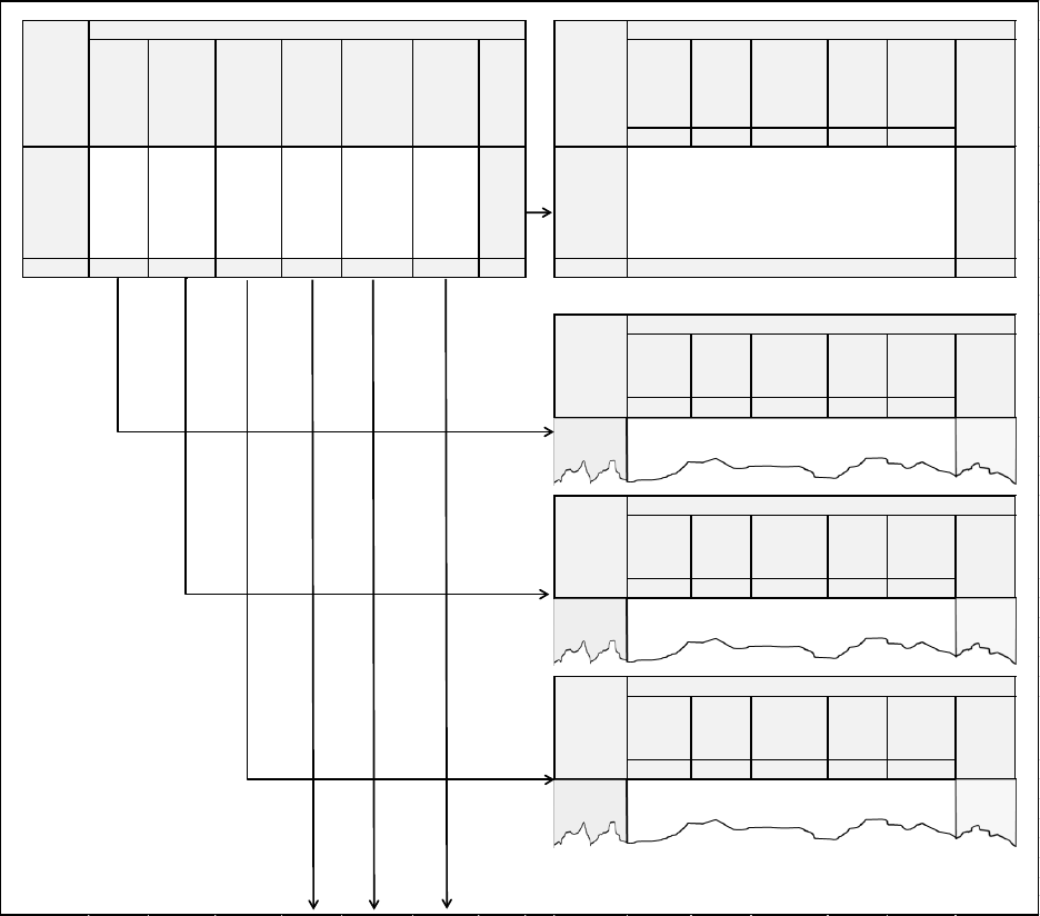
Handbook on Supply and Use Tables and Input-Output Tables with Extensions and Applications
185
Table 6.10 Table linking gross fixed capital formation by industries, assets and products
6.110. In countries where such level of detail data is not available, the product flow approach may
be applied, using assumptions linking the output of a product to the destination of the product in
terms of its purpose. This is a less optimal approach but allows output and demand to be matched.
6.111. It is important to note that gross fixed capital formation – like other product-based variables
in the use table – is valued at purchasers’ prices. It is recorded, however, by including any non-
deductible VAT and excluding any deductible VAT. This will have an impact on those industries
and products to which exemption applies and will be consistent with the valuation of the
intermediate inputs for the corresponding industries.
6.112. In its simplest version, the use table may show gross fixed capital formation as a single
column, and this would also fulfil the requirements for compiling SUTs and some users’ needs.
The single column approach may be preferred if information on gross fixed capital formation is
Gross fixed capital formation by type:
Gross fixed capital formation by industries and type of assets
GFCF
Dwellings
Other
buildings
and
structures
Machinery
and
equipment
Weapon
systems
Cultivated
biological
ressources
Intellectual
property
products
Total
Agriculture
Forestry
and
logging
Fishing and
aquaculture
. . .
Activities of
households
as
employers
Total
PRODUCTS
PRODUCTS ISIC 01 ISIC 02 ISIC 03 . . . ISIC 97
1
1
2
2
.
.
.
.
N N
Total
Total
Agriculture
Forestry
and
logging
Fishing and
aquaculture
. . .
Activities of
households
as
employers
Total
PRODUCTS
ISIC 01 ISIC 02 ISIC 03 . . . ISIC 97
1
2
Agriculture
Forestry
and
logging
Fishing and
aquaculture
. . .
Activities of
households
as
employers
Total
PRODUCTS
ISIC 01 ISIC 02
ISIC 03 . . . ISIC 97
1
2
Agriculture
Forestry
and
logging
Fishing and
aquaculture
. . .
Activities of
households
as
employers
Total
PRODUCTS
ISIC 01 ISIC 02
ISIC 03 . . . ISIC 97
1
2
E.T.C
Gross fixed capital formation
Gross fixed capital formation
GFCF, Dwellings
GFCF, Other buildings and structures
GFCF, Machinery and equipment
Handbook on Supply and Use Tables and Input-Output Tables with Extensions and Applications
186
missing or incomplete. It should, however, be possible to distinguish between broad groups of
assets based on the product classification used in the SUTs framework.
6.113. The quality of the product breakdown is greatly enhanced, however, by the greater level of
detail linking industries, institutional sectors, assets and products. The disaggregation of gross
fixed capital formation by industries and institutional sectors is also needed to calculate the
consumption of fixed capital by industry, and in turn, the value of non-market producers’ output.
The breakdown can be done by columns that correspond fully to the columns for output and
intermediate consumption. It may, however, be feasible to limit the number of columns in such a
breakdown if precise information from source data is lacking.
6.114. If all combinations of gross fixed capital formation by types, industries and institutional
sectors of a detailed matrix were shown as columns in the use table, these columns would
completely dominate the presentation. Furthermore, a disproportionate share of the resources
needed to balance the SUTs might be required to distribute products between the gross fixed capital
formation columns, and finalization of the SUTs might be delayed unnecessarily.
6.115. One practical solution could be to show columns for a few broad categories of industries.
Another could be to show only columns for different types of capital formation within the SUTs
framework. The breakdown by industries could instead take place outside the central SUTs
framework in a subsystem of investment matrices. Here, gross fixed capital formation by product
from the final balanced version of the use table could be allocated to specific industries and
institutional sectors as a separate process.
6.116. Estimates of gross fixed capital formation by industries have, however, an important role
in the preparation of initial column totals for gross fixed capital formation for the use table.
Furthermore, a preliminary version of gross fixed capital formation by products and industries can
provide the starting point for the gross fixed capital formation columns of the use table.
6.117. Table 6.11 illustrates the gross fixed capital formation by industry and product link to the
gross fixed capital formation column in the use table. In essence, this identifies the producers of
capital goods in the rows and the investing industries in the columns.

Handbook on Supply and Use Tables and Input-Output Tables with Extensions and Applications
187
Table 6.11 Gross fixed capital formation by investing industry
Table based on 2011 figures from Austria
Note: the products “Trade”, “Transport” and “Communication” of table 6.1 are presented together in table 6.11
6.118. The gross fixed capital formation matrix has further roles to play. The calculation of capital
stock data and the calculation of a valuation matrix for non-deductible VAT require an assessment
of gross fixed capital formation by product (by producing industry) and investor (by investing
industry). In the investment matrix, the user concept of capital – and not the owner concept of
capital – should be reflected.
6.119. The assessment of consumption of fixed capital as a component of GVA should be based
on empirical capital stock data. The human-made capital stock is derived from cumulative
investment of the past in buildings, machinery and transport equipment, based on the actual
lifetime of a capital good and allowing for retirements and obsolescence by using the perpetual
investor method (see OECD, 2009).
6.120. Consumption of fixed capital is calculated at the current replacement cost of the net capital
stock. The net capital stock is defined as the financial value of the gross capital stock still in use.
Clearly, it will be easier to estimate these types of matrices on the basis of a rectangular SUTs
system with many disaggregated homogeneous products.
(a) Sources for gross fixed capital formation
6.121. For industries that are covered by business statistics, the source data will usually include
information on purchases and sales of capital equipment. It is normally possible to distinguish
between gross fixed capital formation in buildings, structures, vehicles and machinery and
equipment. Investment in intellectual property products is usually also shown but it is not
necessarily classified by categories that can be used for national accounts. For example, these
sources will often include purchased software and may also show a value for larger software
projects but not all projects produced on own account. The measurement process is further
complicated with the inclusion of acquisitions of patents, franchises and goodwill and the fact that
research and development may or may not be wholly or partially capitalized in the source data and
not necessarily recorded in line with the requirements of national accounts.
Agriculture Manuf acturing Construction
Trade,
transport,
communication
Financial
and
business
services
Other
services
PRODUCTS
(1) (2) (3) (4) (5) (6) (7)
Agricultural products
(1) 128 2 0 4 36 10 180
Manuf actured products
(2) 1 223 7 225 664 5 893 9 124 2 626 26 756
Construction
(3) 828 1 752 224 3 822 15 995 2 534 25 155
Trade, transport, communication
(4) 12 1 206 189 2 280 1 672 684 6 043
Financal and business services
(5) 124 4 331 82 1 324 3 065 2 245 11 170
Other services
(6) 0 0 0 0 0 113 113
Total
(7) 2 314 14 516 1 160 13 323 29 892 8 212 69 418
INV ESTING INDUSTRIES
Total at
purchasers'
prices
INDUSTRIES
Handbook on Supply and Use Tables and Input-Output Tables with Extensions and Applications
188
6.122. The distinction between intermediate consumption and gross fixed capital formation in
business statistics sourced from business accounts may be different from that recorded in the
national account. For example, items such as purchased computer software may be recorded as
current expenditure in business accounts but as gross fixed capital formation in the national
accounts, thus an equal and opposite adjustment is required. There are other conceptual differences
between company accounts and national accounts, such as the following:
• Business accounts may not fully show gross fixed capital formation according to economic
ownership. Some financially leased assets may be included in investment by their legal
owners.
• Sales of existing assets should be treated as a negative gross fixed capital formation valued
at the actual prices obtained by the seller. When the sale takes place between two resident
producers, the positive and negative investment will cancel out for the economy as a whole,
except for costs of change of ownership. In business accounts, the figures for disposals of
assets will often be shown at historical cost while the corresponding cumulated depreciation
is shown as a separate item. The difference is the bookkeeping value of the sold asset. If the
actual price obtained differs from this value, the residual is included in secondary income,
and should be reviewed and adjusted for as appropriate. In practice, it can usually be assumed
that the difference between the negative gross fixed capital formation and the bookkeeping
value of the sold asset is insignificant but there may be important exceptions where figures
from company accounts are misleading.
• In business accounts, it is common practice to treat minor or regular purchases of equipment
as current expenses. Such acquisitions may not always be identifiable in the accounts. For
some big corporations, the threshold for classifying purchases as investment can actually be
high, say, $10,000 or more, but practices may vary between countries owing to differences
in legislation and taxation rules.
• Own account production of capital goods may be capitalized in business accounts. Even if
this is not the case, the accounts may contain information on the value of own account
production. The value shown may not, however, be at basic prices as it may only include the
direct cost of raw materials and wages and salaries attributed to its production, in which case
a correction for indirect costs and gross operating surplus may be appropriate.
• Own account production of intellectual property products may not be directly identifiable in
company accounts. Production of software, databases, research and development and
literary, artistic or entertainment originals may sometimes have been capitalized as
intangible assets in company accounts but may be treated as current expenses. For some
intangibles, gross fixed capital formation may be covered by business surveys. In the absence
of further detail, it is recommended that gross fixed capital formation is estimated based on
the wages and salaries paid for this kind of work with an appropriate mark-up for other
Handbook on Supply and Use Tables and Input-Output Tables with Extensions and Applications
189
expenses and typical gross operating surplus. More details on this matter may be found in
the Handbook on Deriving Capital Measures of Intellectual Property Products (OECD,
2010).
6.123. Information on gross fixed capital formation within general government can usually be
found in government accounts. Many of the above issues are also relevant to investment within
general government. Accounts of central and local government will usually include a level of detail
that reveals the distinction between intermediate consumption and gross fixed capital formation.
Extra-budgetary units within general government may, on the other hand, provide less information
on the nature of their costs as may also be the case for NPISHs.
6.124. Special care should be taken when projects are partially or wholly financed by capital
transfers from outside, for instance from international organizations. In such cases, the accounts
may show values that are net of financing from outside. In national accounts, gross fixed capital
formation should record the full value of such projects.
6.125. The value of investment covered by business accounts will often give an incomplete picture
of total gross fixed capital formation because some industries are only partially covered or lack
information on some types of investment. The initial estimates of gross fixed capital formation
may be prepared within an investment matrix framework that shows investment by industries,
institutional sectors, types and products. In the event that uncertain data and so-called
“guestimates” are used in many cells within such a framework, the framework can indicate the
cells that are badly covered by source data but the cells should definitely contain values.
(b) Gross fixed capital formation by products
6.126. It is recommended that regular business surveys should be used as the key source for gross
fixed capital formation by product, in particular since gross fixed capital formation is an erratic
time series and cannot be modelled easily. If possible, these surveys should be linked to those
collecting details on purchases of goods and services for intermediate consumption, in order to
avoid double-counting or missing expenditure. Surveys of the product structure of gross fixed
capital formation may exist but may not cover all industries. As for intermediate consumption, it
may be possible to find detailed information in the annual reports of enterprises.
6.127. Government accounts contain information providing much more detail than a simple
distribution by main types of investment. This information can, including for investment products,
typically appear in an unsystematic form and it will need to be coded by product categories in
SUTs before it can be used.
6.128. For many industries available information on the product dimension of investment is
limited to a few categories or even non-existent. Initial estimates will therefore require some
common-sense decisions.
Handbook on Supply and Use Tables and Input-Output Tables with Extensions and Applications
190
6.129. In the end, the product structure of gross fixed capital formation will to a large extent be
determined by the availability of investment products within the SUTs framework. In the simplest
case, where other information is unavailable, gross fixed capital formation will alone be
determined by the supply of typical investment products that are largely not used for other
purposes.
6.130. Very few products are used exclusively for gross fixed capital formation. In most cases,
the distribution between intermediate consumption, household final consumption expenditure and
gross fixed capital formation that can be estimated using information from business surveys and
company accounts is uncertain, in particular if the rows of the SUTs represent broad categories of
products. The disaggregation of products can reduce this uncertainty, when the necessary source
data are available. For some products, the distribution may be based on other types of information,
as in the following examples:
• If an official register of motor vehicles is accessible, it may be possible to identify the
changes from year to year in the numbers of different types of cars and lorries by age, size
and ownership. Combined with typical prices for the various groups of vehicles, the register
may be used to estimate household final consumption expenditure together with gross fixed
capital formation by industry of new and used vehicles. Registers may also provide
information to help distribute registration taxes by purpose.
• Similarly, it may be possible to use register information to follow the capital stock, and
change in capital stock for other types of transport equipment.
• Official registers of buildings may also include information on type, size, use and owners
and may be used for the distribution of buildings by purpose. For dwellings and private
commercial buildings that are not completely covered by company accounts or business
surveys, register information can be used in the estimation of the value of investment.
• Information on investment in buildings, transport equipment or specific types of machinery
and investment may be collected by business surveys. Some countries carry out quarterly
and annual business surveys covering gross fixed capital formation and underlying details.
On the other hand, some countries occasionally carry out comprehensive industrial censuses
that may contain information on the use of capital equipment for units that are not covered
by other kinds of statistics.
• Household budget surveys can include information on investment in new dwellings and
capital repairs. In countries with a large informal economy, household budget surveys may
be the most important source for the estimation of investment in buildings, machinery and
equipment in small farms (which may also, however, be included in agricultural censuses),
small retail trade and repair workshops.
Handbook on Supply and Use Tables and Input-Output Tables with Extensions and Applications
191
6.131. Furthermore, the product structure of investment tends to be more volatile than the
structure of input cost structures. Nevertheless and despite its uncertainties, an initial version of
investment by products estimated from the uses side is usually preferred to an estimated
distribution based solely on the supply of specific products.
2. Changes in inventories
6.132. In order to define changes in inventories, it is useful to define first what is covered by
inventories. Inventories are produced assets, consisting of goods and services, that came into
existence in the current period or in an earlier period and that are held for sale, use in production
or other use at a later date (2008, SNA, para. 10.12). Changes in inventories are measured by the
value of the entries into inventories less the value of withdrawals and less the value of any recurrent
losses of goods held in inventories during the accounting period. Some of these acquisitions and
disposals are attributable to actual purchases or sales but others reflect transactions that are internal
to the enterprise (2008 SNA, para. 10.118).
6.133. The change in inventories column in the use table should be underpinned with a matrix
linking, as column headings, the classification of industries (for example, ISIC), and, as row
headings, the product grouping (for example, CPC) as appearing in the SUTs for each type of
asset. Changes in inventories can be analysed by industry and by types of assets, which need to be
linked via CPC in the SUTs as illustrated in Table 6.12.

Handbook on Supply and Use Tables and Input-Output Tables with Extensions and Applications
192
Table 6.12 Table linking change in inventories industries, assets and products
6.134. The change in inventories should separately distinguish the following types of assets:
• Materials and supplies, which consist of all products that an enterprise holds in inventory
with the intention of using them as intermediate inputs into production.
• Work-in-progress, which consists of output produced by an enterprise that is not yet
sufficiently processed to be in a state in which it is normally supplied to other institutional
units.
• Finished goods, which consist of goods produced as outputs that their producer does not
intend to process further before supplying them to other institutional units.
Changes in inventories used for correction from sales and purchases to
output and intermediate consumption
Total
PRODUCTS
1
2
Agriculture
Forestry
and logging
Fishing and
aquaculture
. . .
Ac tiv ities of
households
as
employers
Total
PRODUCTS
ISIC 01 ISIC 0 2 ISIC 03 . . .
ISIC 97
1
2
Agriculture
Forestry
and logging
Fishing and
aquaculture
. . .
Ac tiv ities of
households
as
employers
Total
PRODUCTS
ISIC 01 ISIC 0 2
ISIC 03 . . .
ISIC 97
1
2
Agriculture
Forestry
and logging
Fishing and
aquaculture
. . .
Ac tiv ities of
households
as
employers
Total
PRODUCTS
ISIC 01 ISIC 0 2 ISIC 03 . . . ISIC 9 7
1
2
Agriculture
Forestry
and logging
Fishing and
aquaculture
. . .
Ac tiv ities of
households
as
employers
Total
PRODUCTS
ISIC 01 ISIC 0 2
ISIC 03 . . . ISIC 97
1
2
Agriculture
Forestry
and logging
Fishing and
aquaculture
. . .
Ac tiv ities of
households
as
employers
Total
PRODUCTS
ISIC 01 ISIC 0 2
ISIC 03 . . . ISIC 97
1
2
Changes in inventories, Retail trade
Changes in inventories, Materials and supplies
ASSET
TY PE
Changes in inventories
Finished
goods
Work-in-
progress
Goods for
resale,
w holesale
Goods for
resale, retail
Changes in inventories, Finished goods
Changes in inventories, Work in progress
Changes in inventories, Wholesale trade
Materials
and
supplies
Handbook on Supply and Use Tables and Input-Output Tables with Extensions and Applications
193
• Military inventories, which consist of single-use items, such as ammunition, missiles,
rockets, bombs and other items, delivered by weapons or weapons systems. Some single-use
items such as ballistic missiles highly destructive may be classified as fixed assets in the
sense that they provide deterrence services against aggressors.
• Goods for resale, which are goods acquired by enterprises, such as wholesalers or retailers,
for the purpose of reselling them to their customers.
6.135. Although change in inventories for all asset types appear in the final uses part of the use
table, they also play a role across other parts of the supply table and use table:
• For each industry, intermediate consumption can be calculated as purchases of goods and
services less change in inventories of materials, fuels and raw materials.
• For each industry, output can be calculated as sales plus change in inventories of work-in-
progress and finished goods. Producers of services may actually have inventories of work-
in-progress in the form of projects lasting for more than one accounting period, such as films,
advertising campaigns, legal contracts, and so forth.
6.136. The output value in trade can be calculated as sales less purchases less change in
inventories of goods purchased for resale without any further processing. If a distinction between
wholesale and retail trade is made in SUTs, then the calculation of the output value for each of
these industries requires separate values for the change in inventories of goods for resale.
6.137. For estimating output and intermediate consumption, changes in inventories are usually
estimated by industry and institutional sector. These detailed breakdowns are, however, seldom
shown in the use table.
6.138. It must be noted that the changes in inventories reported by the survey respondents should
be adjusted to comply with national accounts definitions: thus the changes in inventories should
not include any holding gains or losses. Source data may be presented as output and intermediate
consumption instead of sales and purchases. In practice, the data collected may nevertheless
contain values of sales and purchases. These data may be replaced by a correction that uses
inventories that appear in the company accounts. If such changes include any holding gains or
losses, the correct treatment is to remove the original correction for inventory changes and replace
it by a correction that uses inventory changes according to national accounts definitions.
6.139. Statistics based on company accounts usually contain information on inventory changes
and also on stocks of inventories. The value shown for change in inventories will usually include
holding gains and losses and will be misleading if significant price changes take place during the
year. A correction for holding gains and losses can usually be based on the nominal values of
opening and closing stocks, or the book value levels. It will require the availability of adequate
information on price changes during the year. The correction can typically be carried out by the
Handbook on Supply and Use Tables and Input-Output Tables with Extensions and Applications
194
inflation or deflation of opening and closing stocks to the average prices of the year before
calculation of the difference. To calculate constant price values of stock of inventories (and
changes in current prices), these prices values should be broken down by products for which price
indices or volume indicators can be found.
6.140. Annual company accounts may not contain information of opening stocks, in which case
it might be necessary to use values of closing stocks from the previous year as a measure of opening
stocks. As coverage changes and establishments are reclassified, the observed differences between
closing stocks and opening stocks may then need some adjustments at the industry level.
6.141. Given the links between sales, purchases and inventories, along with other variables, it is
recommended that the data on inventories are collected via the same survey questionnaires to
ensure coherence across the variables being collected with the same source and at the same point
in time.
6.142. The Eurostat-OECD Compilation Guide on Inventories (Eurostat and OECD, 2017)
provides more detail relating to compilation issues and guidance.
(a) Estimation of changes in inventories by product
6.143. To fill in the columns for changes in inventories, the totals for this item must be broken
down into changes in inventories for the products used in the SUTs and must be completed as part
of generating the estimates of output and intermediate consumption.
6.144. For some products, the values of changes in inventories may be calculated based on
knowledge of physical opening stocks and closing stocks and information on the development in
prices, for example, for crops and livestock in agriculture and for energy products. The calculation
of changes in inventories should be an integral part of subsystems used to provide the complete
product balances for such products.
6.145. The inventories of most industries include a broad selection of products that are usually
not known from statistical sources. The totals of opening stocks and closing stocks used to
calculate changes in inventories need to be distributed by products based on assumptions on the
product structure for each total. The following are typical examples:
• Inventories of finished goods and work-in-progress can be distributed proportionally with
those outputs of each industry that can appear in inventories of goods. Caution will be needed
on service products.
• Inventories of raw materials and fuels can be distributed proportionally with the use of inputs
of each industry that can appear in inventories.
Handbook on Supply and Use Tables and Input-Output Tables with Extensions and Applications
195
• Inventories of goods for resale can be distributed using various proxies for the product
structure, for example, output or input in specific industries, household final consumption
expenditure in specific COICOP groups or gross fixed capital formation of specific types.
• Values of inventories of specific products may already be known from other calculations.
Such values can be retained as predetermined values.
• Some products, for instance electricity, are not likely to appear in inventories. Services
should only appear in inventories as work-in-progress.
6.146. Calculating the distribution of changes in inventories by products in this way is of course
uncertain and it may be adjusted during the balancing of SUTs. There is also a danger that errors
in source data will not be detected if changes in inventories are used as balancing items or not
subjected to adequate quality assurance. The total of changes in inventories should, at least, only
be adjusted in exceptional cases, where this is believed to be the most realistic solution to a
balancing problem.
6.147. It should be noted that any balancing adjustment to the asset composition of changes in
inventories, or to the total changes in inventories, will affect different parts of the supply table and
use table and will have the same total impact on each of the production, income and expenditure
approaches to measuring GDP. This is because the various components of changes in inventories
feed into the estimation of output and intermediate consumption and, in turn, GVA and final uses,
thus the impact of any adjustment will be equal on production, income and expenditure. It is more
likely that quality adjustments will be made to source data, where such changes will, and should,
change the intermediate consumption and output and, in turn, GVA of the corresponding
industries.
3. Acquisitions less disposals of valuables
6.148. Valuables are produced goods of considerable value that are not used primarily for
purposes of production or consumption but are held as stores of value over time (2008 SNA, para.
10.13). Valuables include precious metals and stones, antiques and other art objects and other
valuable items. Acquisitions less disposals of valuables capture these alternative forms of
investments. Capital formation in valuables usually needs to be based on the domestic supply of
specific goods, that is, imports less exports plus the margin. Valuables are by nature difficult to
distribute across industries (based on establishments) as they share certain properties with financial
assets, and the industry breakdown does not reflect those valuables held by, for example,
households.
6.149. Trade data by detailed product provide a good source for identifying such items. Whereas
the margin or fee type data by detailed product may be collected via questionnaires sent, for
example, to auctioneers. For SUTs, the product breakdown is key: thus the relevance of imports
Handbook on Supply and Use Tables and Input-Output Tables with Extensions and Applications
196
less exports by type of product. In terms of the purchaser, this is less important, as the purchaser
could be industry, government or households.
G. Exports
6.150. Exports are shown in the use table by product. Depending on the specific user’s need, an
additional breakdown by column could be provided to show exports by destination. It should be
noted that the treatment, issues and sources of data applied to imports of goods and services are
also applicable to exports of goods and services. More detail on the imports of goods and services
may be found in chapters 4, 5 and 8, including such issues as the new treatment of goods sent
abroad for processing.
6.151. In the use table, exports are valued FOB at the point of exit from the exporter’s economy.
This value includes the cost of transport from the exporter’s premises to the border of the exporting
economy. FOB price includes:
• Value of goods at basic prices
• Trade and transport services to the border
• Taxes minus subsidies on products; there is no VAT on exports
6.152. Since data on exports on goods are collected on a FOB basis, no further transformation is
needed.
1. Data sources
6.153. Most countries have comprehensive foreign trade statistics for goods. Data are generally
collected according to the Harmonized System, valued at FOB and often available with a high
level of detail, say by six-digit or eight-digit Harmonized System codes. Thus the only adjustment
needed to the basic data is the conversion between Harmonized System codes and CPC. It is
usually possible to convert the data from the Harmonized System classification using a
correspondence table from the United Nations website
(http://unstats.un.org/unsd/class/default.asp), supplemented by a conversion table that defines the
SUTs products as aggregates of CPC classifications.
6.154. Various adjustments would be needed to move the foreign trade statistics on to a balance
of payments basis in line with BPM 6, such as the change in economic ownership and the
difference crossing the border.
6.155. Foreign trade statistics will also usually include the distribution of exports of goods by
countries for all products.
6.156. Enterprises with exports below certain threshold values can be allowed to report their
foreign trade without a distribution by products, for example with survey-based external trade
Handbook on Supply and Use Tables and Input-Output Tables with Extensions and Applications
197
statistics. In this case, the values of exports by products will need to be grossed up to cover total
exports. The difference between grossed-up and reported values is uncertain, and may need to be
corrected during the balancing of SUTs. As for inputs, information on the reported values can be
shown together with the grossed-up values in the tables presented to those working on the manual
balancing of SUTs before any automated balancing process.
6.157. The main source for data on exports of services is the balance of payments-based data and
the sources used to produce these data. The classification according to the EBOPS 2010 (United
Nations et al. 2011 and IMF, 2009) will usually provide sufficient detail for conversion into the
classification used in the SUTs. Failing this, access may be available to statistics that show imports
and exports by industries. A conversion into detailed SUTs-based products can be established
based on the coding in balance of payments and the information on the industry classification of
exporting units.
Handbook on Supply and Use Tables and Input-Output Tables with Extensions and Applications
198
Annex A to chapter 6: Sample questionnaire collecting purchases of goods and
services for intermediate consumption
A6.1 The extract shown in Figure A6.1 is from a business survey questionnaire from the
Statistical Office of Serbia. The data are collected for each industry and by product covering the
following:
• Cost of materials
• Closing stocks of materials and fuels
A6.2 Full coverage of goods and services consumed as intermediate consumption to calculate
the industry totals is achieved via further tables collecting data on the costs of industrial and non-
industrial services, an extract from which is shown in figure A6.2. These data make it possible to
calculate the intermediate consumption by product required to populate the intermediate use part
of the use table, as shown in table 6.1.

Handbook on Supply and Use Tables and Input-Output Tables with Extensions and Applications
199
Figure A6.1 Extract from questionnaire covering costs and closing stocks of raw materials
and other material inputs
No.
Code
Product description
Cost of
materials
(group of
account 5.1)
Closing stocks
(group of
accounts 10)
1
2
3 4
5
3000
TOTA L
A GRICULTURA L PRODUCTS, RA W A ND UNPROCESSED PRODUCTS OF PLA NT A ND A NIMAL ORIGIN
3001
01.11.1 - 01.11.4 Cereals, all kinds (except rice), cereal seeds
3002
01.11.6 - 01.11.7 Green leguminous vegetables (beans, peas, lentils and other)
3003
01.11.8
Soya beans, groundnuts (row ) and cotton seed
3004
01.11.9
Other oil seeds - sunflow er, sesame, lin etc.
3005
01.11.12 Rice, not husked
3006
01.13 except 01.13.7
Vegetables, raw
3007
01.13.7
Sugar beet and sugar beet seed
3008
01.13.8 Mushrooms and truff les
3009
01.15 Unmanuf actured tobacco
3010
01.16 Fibre crops (lin, cotton and other f ibre crops, used in textile industry)
3011
01.19.1 Forage crops and vegetative matter for livestock feeding unprocessed form
3012
01.19.2
Flow ers and flow er seeds
3013
01.21
Grapes
3014
01.22 - 01.23
Tropical and subtropical fruits (citrus, figs etc.)
3015
01.24, 01.25 except 01.25.3
Other fruits, tree and bush fruits, except nuts (apples, pears, cherries, berries etc.)
3016
01.25.3 Nuts (almonds, hazelnut, w alnuts etc.)
3017
01.26
Olives, coconuts (row , unprocessed)
3018
01.27
Coff ee beans, tea leaves, cocoa beans, not roasted
3019
01.28 Spices, aromatic, drug and pharmaceutical crops
3020
01.11.5, 01.14, 01.19.3,
01.29, 01.3
Vegetables and fruit seeds, other seeds, grass, unprocessed straw and other residues of cereals, seeds
for trees and seedings, planting materials, sugar cane and other raw , unprocessed and untreated products
of plant origin n.e.c.
3021
01.4. except 01.45.3 &
01.49.3
Live animals and raw animal products (unprocessed milk, eggs, natural honey, except raw skins, shorn
w ool and skins, see line 3022, etc.)
3022
01.45.3, 01.49.3
Raw fur skins, shorn w ool, skins (excluding products of slaughterhouses and industrial meat production,
see 1036)
3023
01.49. part
Other animal products, raw , unprocessed an untreated
3024
01.7
Hunting and trapping products, raw
PRODUCTS OF FORESTRY
3025
02.2
Wood in the rough - logs, f uel w ood and other row products of forestry
3026
02.1, 02.3
Forest trees and seeds, w ild grow ing edible products; natural cork, varnish, balsams and other raw
products of f orestry n.e.c.
FISH A ND OTHER FISHING PRODUCTS, UNPROCESSED A ND UNTREATED
3027
03
Fish and other f ishing products; aquaculture products (raw , unprocessed and untreated)
MINING A ND QUA RRY ING PRODUCTS; UNPROCESSED
3028
05.1, 05.2
Coals, hard coal and lignite
3029
06.1
Crude petroleum, bituminous or oil shale and tar sands. Note petroleum products - fuels are entered in the
row 3118
3030
06.2
Natural gas, processed (Manufactured gas distributed though mains, heating gas and petroleum gases f rom
ref ineries should be reported in row s 3116 and 3119)
3031
07.1
Iron ores
3032
07.2
Other metal ores
3033
08.1 Stone, sand, and clay and other raw materials f or construction, industrial and craft activities
3034
08.9 Other mining and quarrying products n.e.c.
MA NUFA CTURING INDUSTRY PRODUCTS
Food products and other processed products of plant and animal origin; used as reproduced material
3035
10.11 except 10.11.4 &
10.12.5
Meat (red meat, including frozen) except live animals and unprocessed and untreated products of animal
origin (goes to row s 1021 -1024); raw offal and edible fat and oils
:::::::
:::::::
:::::::
:::::::
:::::::
Electricity, ref ined petroleum products for energy purposes, gas (excluding natural gas), steam, hot w ater,
air conditioning (including energy products use for heating)
Account 513
3115
35.11 Electric ity costs
3116
35.22
Manufactured gas for industrial purposes and for heating - gas distributed through mains (excluding natural
gas, see 3030, petroleum gas f rom ref ineries, see 3119 and industrial and medical gases, see 3069)
3117
35.30 Steam and hot w ater, air conditioning supply services
3118
19.2
Refined petroleum products - motor, engine and other fuels
3119
19.2 Petroleum gases - propane, butane etc. (excluding natural gas and industrial and medical gases)

Handbook on Supply and Use Tables and Input-Output Tables with Extensions and Applications
200
Figure A6.2: Extract from questionnaire covering costs of industrial and
non-industrial services
No. CPA code Product description
Costs of
services
Account code
1 2 3 4 5
4000 TOTA L
Support services directly linked w ith the production of goods and services
4001
01.6 part Support agricultural services to crop production
4002
01.6 part Support services to animal production; veterinary services excluded (row 4044)
4003
02.10.2, 02.4 Support services to forestry
4004
09 Mining support services; services to petroleum and natural gas extraction
4005
13.3 Textile finishing services–bleaching, dyeing, printing etc.
4006
16.10.9
Drying, impregnation or chemical treatment services of timber and product of w ood; support services in the
processing of w ood and w ood products n.e.c.
4007
25.5 Forging, pressing, stamping and roll-forming services of metal
4008
25.6 Treatment and coating services of metals, machining
4009
24.5 Casting services of metal and steel
Subcontracted services in industry and construction, trade services and other intermediation commissions.
Note: enter only the value of the services, value of materials of goods excluded
4010
14, part Subcontracted operations in textile industry (excluding value of materials)
4011
15, part Subcontracted operations in footw ear and leather production industry (excluding value of materials)
4012
16, part Subcontracted operations in production of processed w ood and w ood products (excluding value of materials)
4013
25, part
Subcontracted operations as part of machine industry–processing and finishing materials services
(excluding value of materials)
4014
41, 42, 43 Subcontracted operations in construction
4015
–
Other subcontracted operations in production of goods of other enterprises (excluding value of materials),
please specify
4016
46.1 Trade commissions
4017
– Other intermediation commissions,
please specify
Transportation costs, postal and courier services
4018
49
Land transport of freight, taxi operation services including rental services of land transport vehicles w ith
operator
4019
50 Water transport
4020
51 Air transport
4021
52.2
Support services f or transportation (loading, unloading, hauling, tow ing, parking services, etc.,
transportation excluded)
4022
53 Postal services under universal obligation
4023
53 Other postal and courier services
Repair, maintenance, installation services; conversion, reconstruction and fitting out of transport equipment
4024
33.1
Repair and maintenance services of f abricated metal products, machinery and equipment, except motor
vehicles
4025
43 Repair and maintenance services of buildings and electrical, plumbing, heating and similar installations
4026
45.2 Maintenance and repair services of motor vehicles
4027
95.1 Maintenance and repair services of computers and communication equipment
4028
95.2 Repair services of personal and household goods
4029
33.2 Installation services of industrial machinery and equipment
4030
29.20.4, 29.20.5
Reconditioning, assembly, f itting out and bodyw ork services of motor vehicles, except installation,
maintenance and repair services
4031
30.11.9, 30.20.9, 30.30.6
Conversion, reconstruction and fitting out services of other transport equipment, except installation,
maintenance and repair services
Rentals, rents on land, w arehousing and storage services
4032
68.2, part Rental costs on buildings and off ice space ow ned by legal persons (except rents on land)
4033
68.2, part Rental costs on buildings and off ice space ow ned by natural persons (except rents on land)
4034
68.2, part Rents on private land
4035
68.2, part Rents on public or state land
4036
77
Rental and leasing services of motor vehicles, machinery, equipment and tangible goods (excluding real
estate and financial lease)
:::::::
:::::::
:::::::
:::::::
:::::::
Expenditure related to the intellectual property (royalties, licence f ees, rights of usage, publication,
reproduction, transmission, broadcasting and the like), other services n.e.c. Note: services as
expenditures; if not capitalised
4089
58,1 Royalties for the publication of books, magazines, new spapers, etc.
4090
58,2 Royalties and similar payments for usage of softw are
4091
59 Royalties for publishing (music and movies, TV series)
4092
60 Royalties (broadcast rights, etc.) in the production and broadcast of radio and television programs
4093
71,2 Certification of products and processes
4094
77,4 Royalties and fees for the use of intellectual property if it is not capitalised
4095
96,01 Laundry and w ashing of textile and fur
4096
– Other industrial and non-industrial services not elsew here specified
please specify
539 or 559
532
533
530
530, 539
531
Handbook on Supply and Use Tables and Input-Output Tables with Extensions and Applications
201
Annex B to chapter 6: Impact of capitalizing the costs of research and
development in SUTs and IOTs
A. Research and development as fixed capital formation
B6.1 The 2008 SNA introduced changes relating to the treatment of research and development.
Research and development is creative work undertaken on a systematic basis in order to increase
the stock of knowledge, including knowledge of people, culture and society, and to enable this
stock of knowledge to be used to devise new applications. The 2008 SNA does not treat research
and development activity as an ancillary activity and it recommends that a separate establishment
should be distinguished for research and development when possible.
B6.2 The output of research and development should be capitalized as “intellectual property
products” except where it is clear that the activity does not entail any economic benefit to its
producer (and hence owner), in which case it is treated as intermediate consumption.
B6.3 The 2008 SNA now includes expenditures for both bought-in and own-account research
and development as gross fixed capital formation and the depreciation of these assets as
consumption of fixed capital.
B6.4 Table B6.1 shows a summary of the impact of these changes using a simplified hypothetical
example simply to demonstrate the impact of capitalization. The example is simplified in the sense
that it shows only two years and the capitalization of research and development (R&D) is assumed
to be introduced in year 1, when there is no increase in the consumption of fixed capital. In reality,
the capitalization costs will be spread over several successive years and the consumption of fixed
capital will occur in year 1 and throughout the lifetime of the asset.
B6.5 Under 1993 SNA, own-account R&D activity was treated as an ancillary activity and no
separate output was estimated in the system, and expenditures for this purpose were not separately
identified. Only in those cases, usually unimportant, where R&D services were purchased from
outside specialist producers, classified in the research and development activity (ISIC Rev. 4,
division 72) or imported, do R&D services appear in the SUTs as intermediate consumption.
B6.6 With the capitalization of R&D expenditures under the 2008 SNA, the output of own-
account R&D is separately estimated and allocated to GCF or exports. In practice, the introduction
of own-account R&D output in the system has just resulted in additional output with the
intermediate inputs being left unaffected, as the intermediate inputs needed to produce the own-
account R&D were already included. With the 2008 SNA change of treating research and

Handbook on Supply and Use Tables and Input-Output Tables with Extensions and Applications
202
development not as an ancillary activity, the question for the compilation of SUTs and IOTs is
whether the R&D output from own-account R&D activity should be seen as a secondary product
from that particular branch or the principal product of the activity “Scientific research and
development” ISIC Rev. 4, division 72. This issue of reclassification of own-account R&D activity
is considered in the following section.
B6.7 The challenging methodological and practical problems related to the actual estimates of
output of own-account research and development are not being dealt with at this point; reference
is made to the Manual on Measuring Research and Development in ESA 2010 (Eurostat, 2014a),
the Handbook on Deriving Capital Measures of Intellectual Property Products (OECD, 2010) and
specific country documentations. In the following, only some problems of special interest for the
compilation of SUTs and IOTs will be highlighted.
Table B6.1 Summary of the impact of the capitalization of research and development in the
new 2008 SNA
For own account value of production is 1000. For non-market producers, consumption of fixed capital in
Year 2 is 200.
For bought-in, value of intermediate consumption is 500. For non-market producers, consumption of fixed
capital in Year 2 is 100.
Year 1 estimates. Estimates in brackets to relate to consumption of fixed capital to impact in Year 2 for
non-market producers.
B. Implications of valuation of output as sum of costs
B6.8 Output for own final use should be valued at the basic prices at which the goods and
services could be sold if offered for sale on the market. When reliable market prices cannot be
obtained, a second best procedure must be used, in which the value of the output of the goods or
services produced for own final use is deemed to be equal to the sum of their costs of production,
that is, as the sum of: intermediate consumption; compensation of employees; consumption of
fixed capital; a net return to fixed capital; and other taxes (less subsidies) on production. By
Ow n
account
Bought-in
(1) (2)
Intermediate consumption 0 -500 0 -500
Non-market consumption of f ixed capital 0 0 (+200) (+100)
Gross operating surplus +1 000 +500 (+200) (+100)
GVA +1 000 +500 (+200) (+100)
Total output +1 000 0 (+200) -500 (+100)
Output f or ow n fnal use +1 000 0 +1 000 0
General governemnt or NPISHs final
consumtpion expenditures
0 0 -1 000 (+200) -500 (+100)
Gross fixed capital formation +1 000 +500 +1 000 *500
Impact on GDP +1 000 +500 0 (+200) 0 (+100)
(3)
(4)
Indicative impact
Change in the treatment of Research and Development
Market producers
Non-market producers
Ow n account
Bought in
Handbook on Supply and Use Tables and Input-Output Tables with Extensions and Applications
203
convention, no net return to capital is included when own-account production is undertaken by
non-market producers (2008 SNA, para. 6.125).
B6.9 The calculation of the output of own-account R&D from the sum of costs approach means
that the cost structure for this particular type of output will be separately specified; this is a
departure from the usual situation where intermediate and primary inputs used for various types of
outputs will be indistinguishably lumped together. Based on the known cost structure, it would in
principle be possible to create separate establishments for the own-account R&D activity, and if
further on this activity was seen as secondary, to reclassify these establishments from the original
activity to which they are classified, for example, pharmaceuticals, electronics and so forth, to the
specialist activity for scientific research and development (ISIC Rev. 4, division 72).
B6.10 For a number of analytical, methodological and practical reasons, however, such a
reclassification is not recommended. These reasons include, primarily, the following:
• There is an analytical interest in keeping track of those economic activities that actively
involve R&D and this information would be lost through such a reclassification.
• As each R&D output is uniquely defined, the own-account research and development is
usually not suitable for delivery outside the producing unit, and a reclassification would not
reflect the economic reality of the activity.
• Given the lack of any other information, it is assumed that the producing unit is also the
owner of the resulting R&D capital stock and the associated consumption of fixed capital –
this assumption is often not valid.
• The cost structures calculated to derive the estimate of R&D output will not usually have
product details corresponding to the SUTs product requirement, and in general, will only
exist as internal worksheet exercises not intended for a wider audience.
• If all R&D were reclassified to ISIC Rev. 4, division 72, in many developed countries this
division would increase to the same size or even larger than the agricultural sector, and
seriously distort the relative proportions, in particular between manufacturing industries and
service industries. It would also make industries active in R&D (such as the pharmaceutical
industry) rather meaningless truncated residuals compared with the usual perception of the
size and structure of these industries and thus the reclassifications would be
counterproductive from the point of view of users’ needs and a wide-range of analytical
purposes.
C. Own-account research and development as principal or secondary output
B6.11 Research and development services, division 81 of CPC Version 2.1, also existed prior to
the capitalization of R&D, and were mainly made up of the services actually sold in the market by
Handbook on Supply and Use Tables and Input-Output Tables with Extensions and Applications
204
enterprises classified in division 72 of ISIC Rev. 4, “Scientific research and development”. This
was generally small, however, when compared with the total value of own-account R&D estimated
in connection with the capitalization.
B6.12 In division 81 of CPC Version 2.1, the subclasses are organized according to the type of
research (for example, chemistry, biotechnology, and others), and not according to the economic
activities carrying out the R&D, and all R&D services are indicated as characteristic products of
ISIC Rev. 4 subclasses 7210 and 7220. This follows logically from the fact that CPC Version 2.1
was not designed for a situation where the overwhelming share of R&D services comes into
existence as estimated own-account output in ISIC industries other than ISC Rev. 4, division 72.
B6.13 Under the system of estimated own-account output of R&D services, it would be more
appropriate to introduce a CPC structure for R&D similar to the structures for “Maintenance, repair
and installation (except construction) services” (CPC Version 2.1, division 87) and for
“Manufacturing services on physical goods owned by others” (CPC Version 2.1, division 88)
where the subclasses (four digits) are made up industry specific outputs, each corresponding to a
characteristic ISIC class (four digits). This means, in particular, that outputs of these services in
industries which are active in R&D form principal outputs. When this approach is followed for
own-account R&D services, there will be as many subclasses of CPC division 81 as there are
industries with R&D activities, and own-account R&D will formally change from a secondary to
a principal activity of the producing industries. The adoption of this approach will also have
important implications when deriving IOTs from the SUTs, as it will prevent major structural
differences between industry-by-industry IOTs and product-by-product IOTs, and avoid truncating
research and development-intensive product-adjusted industries in the product-by-product IOTs.
B6.14 In practice, specialized R&D departments of enterprises with major own-account R&D
activities may, for various reasons (legal, tax-related, and other), have already been classified in
ISIC Rev. 4, division 72, in the business register, and thus be included in business statistics with
this activity, rather than the principal activity (for example, pharmaceutical, electronic and so
forth) of the parent enterprise.
B6.15 In such cases, the flows between the R&D department classified in ISIC Rev. 4, division
72, and the parent enterprise, and also the applied valuation principles, should be carefully
assessed. In this connection, it is important to realize that business accounting practices will
usually not follow the principle of capitalizing R&D expenditures. Thus the total output (however
estimated) from an R&D department classified in ISIC Rev. 4, division 72, may, in the business
accounts, reappear as intermediate consumption in the accounts of the parent enterprise.
Depending on the circumstances, one solution might be to reclassify the R&D department back to
the activity of the parent enterprise. In national accounts, sometimes legal structures may be
overruled if they are found not to reflect economic realities. Alternatively, the intermediate
consumption of R&D services could simply be removed from the parent enterprise and instead
treated as gross fixed capital formation, but this may leave a truncated enterprise of little analytical
Handbook on Supply and Use Tables and Input-Output Tables with Extensions and Applications
205
interest, as noted above, and it would still be necessary to deal with the valuation of reported output
of the R&D department.
D. Balancing supply and use of research and development services
B6.16 Assuming that the output of R&D services (market, non-market and for own-use) by
industry is available from the current national accounts calculations, allocation by user should, in
principle, be fairly straightforward, as these services under the 2008 SNA treatment of R&D
should be allocated to gross fixed capital formation. There are, however, two problem areas worth
mentioning:
• Some research and development purchases are still to be treated as intermediate
consumption.
• Foreign trade in research and development services must be taken into account when
balancing the R&D services.
B6.17 When market R&D services are purchased by an own-account producer of R&D from a
commercial R&D producer (usually, although not necessarily, classified in ISIC Rev. 4, division
72) or imported, it must be decided whether this is an acquisition of an asset or an intermediate
product used as an input into the own-account production of R&D. As there is usually insufficient
information available on the individual transactions for an informed decision to be made, it is
recommended by the Eurostat Manual that, in the absence of any strong evidence to the contrary,
all purchases by own-account R&D producers from units classified in ISIC Rev. 4, division 72,
(and also purchases by other units in ISIC Rev. 4, division 72) should be treated as intermediate
consumption. This assumption will also ease the distribution in cases where no product statistics
for the output from ISIC Rev. 4, division 72, are available, as some output may be non-research
and development services that would nonetheless usually be allocated to intermediate
consumption.
B6.18 The above-mentioned case involving a specialized R&D department classified in division
72 of ISIC Rev. 4 may, however, interfere with this solution, and it is recommended that the SUTs
compilers coordinate closely with the compilers of the R&D estimates made for the national
accounts.
B6.19 In the 2010 Manual on Statistics of International Trade in Services (United Nations, IMF,
OECD, European Union, UNCTAD, UNWTO and WTO, 2011) and Extended Balance of
Payments Services Classification (EBOPS, 2010), there are special entries on R&D services,
which are explicitly separated from transactions on the results of R&D (for example, royalties and
license fees paid for use of patented entities).
B6.20 It would therefore appear that the balancing of the R&D services, also taking into account
imports and exports, would be straightforward. The transactions registered in the balance of
Handbook on Supply and Use Tables and Input-Output Tables with Extensions and Applications
206
payments are, however, actual economic transactions where the prices may be quite different from
the cost-based valuation of the domestic own-account output of R&D services, and the delimitation
of the R&D concept may also deviate. Further balance of payments transactions in R&D may
include significant elements of transfer pricing and trade with subsidiaries in low-tax jurisdictions.
When the aim is to achieve consistency with existing balance of payments data, the final balancing
of the R&D services may be quite difficult, even though the capitalized R&D services allows trade
in “used” R&D so that gross fixed capital formation may in principle (though no very realistically)
become negative. More detail on these issues may be found in chapter 7 of the guidance on the
impact of globalization on national accounts prepared by the Economic Commission for Europe
(UNECE, 2011).
Handbook on Supply and Use Tables and Input-Output Tables with Extensions and Applications
207
Chapter 7. Compiling the valuation matrices
A. Introduction
7.1. The compilation of valuation matrices is a fundamental step in the process of compiling
SUTs. These matrices are necessary to bridge the different valuation concepts of the product flows.
This chapter covers the main concepts and methods of compiling matrices for trade margins,
transport margins, taxes on products and subsidies on products. In particular, in section B, the
chapter starts with an overview of the valuation concepts in the 2008 SNA and of how the valuation
matrices fit within the SUTs presented in chapters 5 and 6. Sections C–E elaborate on each
component of the valuation matrices and describe the main compilation steps. The annex to this
chapter provides further details on how to compile trade margins for the SUTs from survey data
based on a country practice.
B. Valuation of product flows
7.2. Transactions are valued at the actual prices agreed upon by the purchasers and sellers.
Market prices are thus the main reference for the valuation of transactions in the SUTs system, in
line with 2008 SNA. In the absence of market transactions, the valuation is made according to
costs incurred (for example, for non-market services produced by government) or by reference to
market prices for analogous goods and services (for example, for services of owner-occupied
dwellings).
1. Valuation concepts in the 2008 SNA
7.3. More than one set of prices may be used to value outputs and inputs depending on how
taxes and subsidies on products, trade and transport margins are recorded. The 2008 SNA
distinguishes three main valuation concepts of the flows of goods and services: the two main
recommended valuations being basic prices and purchasers’ prices and the lesser used producers’
prices.
7.4. The basic price is the amount receivable by the producer from the purchaser for a unit of a
good or service produced as output minus any tax payable, and plus any subsidy receivable, by the
producer as a consequence of its production or sale. It excludes any transport charges invoiced
separately by the producer (2008 SNA, para. 6.51).
7.5. The producers’ price is the amount receivable by the producer from the purchaser for a unit
of a good or service produced as output minus any VAT, or similar deductible tax, invoiced to the
Handbook on Supply and Use Tables and Input-Output Tables with Extensions and Applications
208
purchaser. It excludes any transport charges invoiced separately by the producer (2008 SNA, para.
6.51).
7.6. The purchasers’ price is the amount paid by the purchaser, excluding any VAT or similar
tax deductible by the purchaser, in order to take delivery of a unit of a good or service at the time
and place required by the purchaser. The purchasers’ price of a good includes any transport charges
paid separately by the purchaser to take delivery at the required time and place (2008 SNA, para.
6.64).
7.7. The difference between these valuation concepts for a product relates to trade margins,
transport margins and taxes on products and subsidies on products. The relationship between the
three types of prices is as follows:
Basic prices + Taxes on products excluding invoiced VAT
- Subsidies on products
= Producers’ prices
+ Wholesalers’ trade margins
+ Retailers’ trade margins
+ Separately invoiced transport charges
+ VAT not deductible by the purchaser
= Purchasers’ prices
7.8. The basic price measures the amount retained by the producer and, therefore, the price most
relevant for the producers’ decision-making and is often reported in business surveys. For imported
products, taxes on products include import duties. When the relationship between basic prices and
purchasers’ prices is compiled for the total economy, the transport charges and trade margins will
cancel out because they form only a reallocation of value across products.
7.9. The concept of producers’ prices does not form any of the main valuations. The preferred
valuation of output and GVA in the SNA is made at basic prices and for intermediate consumption
at purchasers’ prices. It is worth recognizing that source data from business surveys for sales may
be valued at producers’ prices. In these cases, data should be adjusted to a basic price valuation
before they are entered into the SUTs. If this step is not completed, then a different recording of
taxes on products and subsidies on products must be established, and GVA by economic activity
would be partly at market prices, a practice which is not recommended by the SNA.
7.10. It is important to note that the relationship between basic price and purchasers’ price does
not describe a process over time for an identifiable product. In this case, the difference between
basic prices and purchasers’ prices is likely to contain an element of holding gains and losses while
the product is with the producer and with wholesale and retail traders (2008 SNA, para. 3.148).
The SNA value concepts are consistently defined in such a way that holding gains and losses do
not become part of GVA and GDP. Hence a trade margin is relative to the replace price of the
Handbook on Supply and Use Tables and Input-Output Tables with Extensions and Applications
209
good “at the time it is sold”, and the price of intermediate consumption relates to what the producer
would have to pay to replace it “at the time it is used”.
7.11. The source data used to fill the cells in the SUTs may have different valuations:
• Production and output data are valued at basic prices.
• Intermediate consumption and final uses are valued at purchasers’ prices.
• Imports are valued at CIF prices. This is the valuation of a good delivered at the point
of entry into the importing economy or the price of a service delivered to a resident,
before the payment of any import duties or other taxes on imports or trade and transport
margins within the country. In the SUTs framework, for national SUTs, the CIF value
is taken to be the basic price of imports of goods.
• Exports are valued at FOB prices. This is the valuation of a good at the point of exit
from the exporter’s economy or the price of a service delivered to a non-resident,
including transport charges and trade margins up to the point of the border, and
including any taxes less subsidies on the goods exported. In the SUTs framework, the
FOB value is taken to be the purchasers’ price of exports of goods.
7.12. It is recommended that the different valuation components of the product flows are
separated to ensure that the SUTs framework is balanced in a fully coherent and consistent manner.
One of the purposes of the valuation matrices is to bridge the difference between the valuation at
basic prices and the valuation at purchasers’ prices and to come up with SUTs at basic prices.
Figure 7.1 illustrates how the valuation matrices link the supply table with the use table. They
comprise all flows that are related to the supply and use of trade margins and transport margins
and to taxes and subsidies on products.

Handbook on Supply and Use Tables and Input-Output Tables with Extensions and Applications
210
Figure 7.1 Schematic representation of the valuation matrices in the SUTs
7.13. In the supply table, the valuation matrices consist of columns (the “bridge column” in
Figure 7.1) which transform the supply of each product from basic prices to purchasers’ prices,
and, in turn, match the product values in the use table compiled at purchasers’ prices.
7.14. In the use table, the valuation matrices consist of product-by-industry matrices of trade
margins, transport margins, taxes on products and subsidies on products which allow for the
transformation of the values of the use table from purchasers’ prices into basic prices. The
availability of such matrices makes possible the balancing of SUTs at basic prices and purchasers’
prices and, as recommended in the Handbook, both valuations should be balanced simultaneously.
7.15. Although it is not strictly necessary that a balanced SUTs framework ends up with tables
showing valuation both at purchasers’ and at basic prices, this is recommended for several reasons.
For analytical purposes, the SUTs data must have the same valuation, and usually the basic price
version is the most appropriate. This is also the case for the process of transforming the SUTs into
IOTs and for the volume estimates in a consistent SUTs framework leading to the estimation of
GVA in volume terms, using double deflation.
7.16. For these input-output based analytical purposes, a valuation as uniform as possible of the
cells in a row of the use table is essential. The values at purchasers’ prices in the different uses will
usually be affected by differences in trade and transport margins, and by differences in taxes on
products and subsidies on products, according to the specific user. The uniformity requirement is
therefore best fulfilled by values at basic prices, although the cells valued at basic prices may still
show user specific price variation: this is the most uniform valuation concept that in practice can
be achieved.
Final use
Purchasers' prices
Non-deductible VAT
Other net taxes on products
Trade and transport margins
Use of industries
Basic prices
Total use
Exports
Changes in inventories
Changes in valuables
Purchasers' prices
Gross fixed capital formation
Non-deductible VAT
Final consumption expenditure of government
Other net taxes on products
Final consumption expenditure of NPISH
Trade and transport margins
Final consumption expenditure of households
Industries
Intermediate consumption
Basic prices
Total use
Output
USE
SUPPLY
Products
Total supply
Imports
Bridge
column
for
valuation
Handbook on Supply and Use Tables and Input-Output Tables with Extensions and Applications
211
2. Valuation matrices in the SUTs framework
7.17. The valuation matrices comprise information on trade margins, transport margins, taxes on
products and subsidies on products. Valuation matrices can be established for the supply table
(supply-side valuation matrices) and the use table (use-side valuation matrices). In a balanced
SUTs system, the use-side valuation matrices and the supply-side valuation matrices will add up
to the same totals. In this section, the full set of valuation matrices is described.
(a) Supply-side valuation matrices
7.18. The supply-side valuation matrix consists of a set of columns added to the supply table at
basic prices to derive the supply at purchasers’ prices. These columns comprise trade margins,
transport margins, VAT, taxes on products and subsidies on products. Table 7.1 shows the
structure of the supply table at basic prices, including a transformation into purchasers’ prices. The
table corresponds to table 5.2 of chapter 5 and is reproduced here for ease of reference. The left
part of this table starts with the domestic output of the various industries by products at basic
prices. The inclusion of the imports valued at CIF prices by products generates the total supply by
products at basic prices, as shown in column (9).
7.19. In the supply table, the output at basic prices of trade services (of which trade margins form
the major part) is included in row (4) and that of transport services in row (5). To arrive at
purchasers’ prices for each product, the trade margin and transport margin shares of this output
have to be reallocated from trade margins and transport services to the traded and transported
products. Columns (10) and (11) of Table 7.1 contain the allocation of trade margins and transport
margins respectively, with positive entries (+) in the rows of the traded and transported products
and negative entries (-) in the rows of trade services and transport services. The totals by row of
columns (10) and (11) of trade and transport margins respectively are always zero.
7.20. The columns of taxes less subsidies of products – columns (12)–(14) of Table 7.1 – are
also added to total supply at basic prices in order to arrive at the total supply at purchasers’ prices.
Taxes on products comprise VAT-type taxes, taxes and duties on imports and other taxes on
products. Similarly, subsidies on products comprise import subsidies and other subsidies on
products. Taxes and subsidies on products should be compiled separately although they may be
shown as a single column.
7.21. The addition of columns (10)–(14) to total supply at basic prices of column (9) gives total
supply at purchasers’ prices in column (16). Columns (10) and (14) thus provide the bridge needed
to compare and balance total supply with total use when both sides are valued at purchasers’ prices.
7.22. Both trade margins and transport margins can be produced by any industry outside the trade
and transport industries. The bulk of the output of trade margins, however, is generally produced
by the trade industries and the bulk of transport margins by the transport industries, as illustrated
in rows (4) and (5) of Table 7.1.

Handbook on Supply and Use Tables and Input-Output Tables with Extensions and Applications
212
Table 7.1 Supply table at basic prices, including a transformation into purchasers’ prices
Millions of euros
Table based on 2011 figures from Austria
(b) Use-side valuation matrices
7.23. The use-side valuation matrices consist of a sequence of matrices – mirroring the shape of
the intermediate use and final use parts of the use table – for each component of the valuation,
namely, for trade margins, transport margins, taxes on products and subsidies on products.
7.24. Table 7.2 illustrates the use table at purchasers’ prices. This table corresponds to table 6.1
of chapter 6 and is reproduced here for ease of reference. It shows the structure of the table,
comprising the following three sub-matrices:
Agriculture Manufacturing Construction
Trade,
transport and
communication
Finance and
business
services
Other
services
(1)
(2) (3)
(4)
(5) (6)
(7) (8) (9)
Agriculture
(1) 8 782
0 0 0 0 0 8 782
3 271
12 052
Manufacturing (2) 796 182 982 643 1 808
133
44 186 405 124 590
310 995
Construction (3) 83
961 43 060 734 255 179
45 272 563 45 835
Trade (4) 1 4 773 311 54 204 640 257 60 187
600 60 787
Transport (5) 13 465 66 25 538 128 125 26 335 8 150 34 485
Communication (6) 160 1 781 139 43 912 1 253 982 48 228 6 234 54 463
Finance and business services (7) 29 8 902 698 7 588 106 909 3 381 127 508 7 061 134 569
Other services (8) 3 85 13 1 053 143 74 346 75 643 824 76 467
Total (9) 9 867 199 950 44 931 134 837 109 461 79 314 578 360 151 293 729 653
CIF/FOB adjustments on imports (10) 0
0 0
0
0 0
0 - 97 - 97
Direct purchases abroad by residents (11) 0 0 0 0 0 0 0 6 675 6 675
Total (12)
9 867 199 950 44 931 134 837
109 461 79 314 578 360
157 871 736 230
Total of w hich:
Market output (13) 9 763
195 916 41 462 127 401 88 330 18 116
480 989 0
Output for ow n final use (14)
104 4 029
3 468 2 134 19 890
2 670 32 295
0
Non-market output (15) 0 4 0 5 302
1 241 58 528 65 075
0
Trade margins
Transport
margins
VAT
Taxes on
products
Subsidies
on products
Total
(9) (10) (11)
(12) (13) (14) (15) (16)
Agriculture (1)
12 052 1 926 274 329
57 - 107 2 479
14 532
Manufacturing (2) 310 995 48 838 2 540 13 175
7 866 - 49 72 370 383 364
Construction (3) 45 835
0 0
1 529
13 0 1 542 47 377
Trade (4)
60 787 - 52 341 0
575 11 0
- 51 755 9 032
Transport (5) 34 485
0 - 2 800 558 71 - 448 - 2 620
31 865
Communication
(6) 54 463 1 493 9 3 375 217 - 34 5 059 59 522
Finance and business services (7) 134 569 0 - 22 2 706 2 159 0 4 842 139 411
Other services (8) 76 467 85 0 1 201 576 0 1 861 78 329
Total (9) 729 653 0 0 23 447 10 969 - 638 33 778 763 431
CIF/FOB adjustments on imports (10) - 97
0 0 0 0
0 - 97 - 97
Direct purchases abroad by residents (11) 6 675 0 0 0 0 0 6 675
6 675
Total (12)
736 230 0 0 23 447
10 969 - 638 40 356 770 009
Total of w hich:
Market output (13)
0 0 0
0 0 0
0 0
Output for ow n final use (14) 0 0 0 0 0
0 0 0
Non-market output (15)
0 0 0 0 0 0 0 0
Adjustments
INDUSTRIES
Output
at basic
prices
Imports
Total supply
at basic
prices
PRODUCTS
Total supply
at basic
prices
V A LUA TION MA TRICES
Total supply
at
purchasers'
prices
PRODUCTS
Adjustments

Handbook on Supply and Use Tables and Input-Output Tables with Extensions and Applications
213
• Intermediate consumption matrix showing intermediate consumption for each industry by
product
• Final uses matrix showing final uses by type of final use and by product
• GVA matrix showing the components of GVA for each industry
Table 7.2 Use table at purchasers’ prices
Millions of euros
Table based on 2011 figures from Austria
7.25. The matrices covering intermediate consumption and final uses are valued at purchasers’
prices, thus they include trade margins and transport margins, along with taxes on products less
subsidies on products. Accordingly, the sum of total intermediate consumption at purchasers’
prices (column (7) of Table 7.2) and total final use (column (15) of Table 7.2) gives the total use
by product at purchasers’ prices, which, in a balanced system, is equal to the total supply by
products at purchasers’ prices in column (16) of the supply table in Table 7.1.
7.26. Table 7.3 shows the use-side valuation matrices covering trade margins (split between
wholesale and retail trade margins), transport margin, VAT, taxes on products and subsidies on
products. These matrices have the same structure and dimension as the intermediate consumption
and final uses sub-matrices of the use table at purchasers’ prices. They show the allocation of the
trade margins, transport margins, taxes and subsidies on products to each element of the use table
at purchasers’ prices. They represent the amounts that must be deducted from each element of the
use table at the purchasers’ price in order to arrive at the use table at basic prices.
Households NPISH
General
government
(1) (2)
(3) (4) (5) (6) (7) (8) (9) (10) (11) (12) (13) (14) (15) (16)
Agriculture
(1) 2 583 6 570 16 371 34 49 9 623 3 595 0 0 180 0 - 27 1 161 4 909 14 532
Manufacturing (2) 2 205 107 190 12 441 16 874 6 015 8 797 153 522 71 438 0 3 180 26 756 2 183 3 034 123 252 229 842 383 364
Construction (3) 105 2 440 9 528 2 446 3 907 1 604 20 029 1 667 0 0 25 155 0 - 38 563 27 348 47 377
Trade (4) 33 1 883 119 2 240 259 308 4 842 3 325 0 0 67 45 0 753 4 189 9 032
Transport (5) 14 4 386 267 8 399 822 321 14 208 5 833 0 3 370 0 0 0 8 453 17 656 31 865
Communication (6) 34 2 563 299 9 359 5 919 1 833 20 008 26 444 0 121 5 976 0 67 6 905 39 514 59 522
Finance and business
services
(7) 457 13 578 4 736 20 359 29 166 9 134 77 430 38 838 0 1 006 11 170 0 - 178 11 145 61 981 139 411
Other services (8) 8 382 59 1 171 415 1 794 3 829 14 923 5 416 53 373 113 107 1 567 74 500 78 329
Total at purchasers’ prices
before adjustments
(9)
5 440
138 991 27 466 61 219 46 538 23 839 303 492 166 063 5 416 61 050 69 418 2 335 2 859 152 800 459 939 763 431
CIF/FOB adjustments on
exports
(10)
0
0 0 0 0 0 0 0 0 0 0 0 0 - 97 - 97 - 97
Direct purchases abroad by
residents
(11)
0 0 0 0 0 0 0 6 675 0 0 0 0 0 0 6 675 6 675
Purchases in the domestic
territory by non-residents
(12)
0 0 0 0 0 0 0 - 12 945 0 0 0 0 0 12 945 0 0
Total at purchasers’ prices (13) 5 440 138 991 27 466 61 219 46 538 23 839 303 492 159 792 5 416 61 050 69 418 2 335 2 859 165 648 466 517 770 009
Compensation of employees (14)
551 30 679 10 239 37 906 22 997 41 971 144 343 0 0 0 0 0 0 0 0 0
Other taxes less subsidies
on production
(15) - 1 627 1 077 546 1 755 2 004 1 103 4 858 0 0 0 0 0 0 0 0 0
Consumption of fixed capital (16) 1 845 12 750 1 542 10 917 18 934 7 480 53 469 0 0 0 0 0 0 0 0 0
Net operating surplus/Net
mixed income
(17) 3 658 16 453 5 138 23 040 18 989 4 921 72 198 0 0 0 0 0 0 0 0 0
Gross operating
surplus/gross mixed income
(18) 5 503 29 203 6 680 33 957 37 923 12 401 125 667 0 0 0 0 0 0 0 0 0
GVA (19) 4 427 60 959 17 465 73 618 62 923 55 475 274 868 0 0 0 0 0 0 0 0 0
Total input at basic prices (20) 9 867 199 950 44 931 134 837 109 461 79 314 578 360 0 0 0 0 0 0 0 0 0
PRODUCTS
Adjustments
GVA
Final consumption expenditure
Gross f ixed
capital
formation
Total use at
purchasers’
prices
Agricul-
ture
Manufac-
turing
Construc-
tion
Trade,
transport and
communication
Finance and
business
services
Other
services
Total
Changes in
valuables
Changes in
inventories
Exports
Total
INDUSTRIES
FINA L USE

Handbook on Supply and Use Tables and Input-Output Tables with Extensions and Applications
214
Table 7.3 Use-side valuation matrices
Table based on 2011 figures from Austria
7.27. It should be noted that the use-side valuation matrices in Table 7.3 relate to the supply-side
valuation matrices in Table 7.1 as follows:
Households NPISH
General
government
(1)
(2) (3) (4) (5) (6) (7) (8) (9) (10) (11) (12) (13) (14) (15) (16)
Agriculture (1) 31 440 2 63 4 6 547 326 10 4 165 506 1 052
Manufacturing (2) 164 6 450 1 415 1 879 326 1 049 11 284 5 941 560 2 718 15 265 8 995 18 493 29 777
Construction (3)
Trade (4) - 196 - 6 910 - 1 420 - 1 997 - 367 - 1 082 - 11 972 - 6 464 - 569 - 2 776 - 15 - 273 - 9 232 - 19 329 - 31 301
Transport (5)
Communication (6) 0 20 3 55 37 27 141 197 9 48 4 72 330 472
Finance and business services (7)
Other services (8)
Total (9) 0 0 0 0 0 0 0 0 0 0 0 0 0
Agriculture (1) 3 0 13 0 1 17 856 856 873
Manufacturing (2) 19 56 20 339 38 90 562 16 781 477 1 142 99 18 499 19 061
Construction (3)
Trade (4) - 19 - 86 - 25 - 431 - 104 - 150 - 815 - 18 363 - 511 - 1 168 - 184 - 20 226 - 21 040
Transport (5)
Communication (6) 0 27 5 79 66 59 236 725 34 26 785 1 021
Finance and business services (7)
Other services (8) 85 85 85
Total (9) 0 0 0 0 0 0 0 0 0 0
Agriculture (1) 7 201 1 7 0 1 217 44 2 1 11 57 274
Manufacturing (2) 20 1 125 191 127 30 64 1 557 303 21 144 2 26 486 983 2 540
Construction (3)
Trade (4)
Transport (5) - 27 - 1 321 - 191 - 135 - 31 - 65 - 1 771 - 347 - 21 - 146 - 2 - 27 - 487 - 1 030 - 2 800
Communication (6) 0 0 1 1 0 4 3 0 2 0 1 5 9
Finance and business services (7) 0 - 5 - 1 - 1 0 0 - 7 - 3 0 - 2 0 0 - 10 - 15 - 22
Other services (8)
Total (9) 0 0 0 0 0 0 0 0 0 0 0 0 0 0 0
Agriculture (1) 0 0 0 0 0 3 4 324 1 325 329
Manufacturing (2) 18 71 18 68 200 942 1 317 10 624 368 734 132 11 858 13 175
Construction (3) 0 1 7 4 242 185 439 265 825 1 090 1 529
Trade (4) 3 16 4 20 17 39 100 467 2 7 476 575
Transport (5) 0 1 0 9 8 17 36 487 34 521 558
Communication (6) 0 1 0 16 207 150 374 2 888 10 103 3 001 3 375
Finance and business services (7) 0 3 3 28 561 713 1 308 1 235 163 1 398 2 706
Other services (8) 0 0 0 1 17 44 63 921 209 8 1 138 1 201
Total (9) 22 93 32 147 1 252 2 093 3 639 17 210 621 1 830 147 19 807 23 447
Agriculture (1)
0 50 0 1 0 0 51 5 1 0 0 6 57
Manufacturing (2) 62 834 179 1 068 212 544 2 898 4 272 6 284 5 7 393 4 968 7 866
Construction (3) 0 1 3 1 1 0 5 0 7 8 13
Trade (4) 0 5 0 4 0 0 10 1 0 0 1 11
Transport (5) 0 7 1 8 11 3 30 26 0 14 40 71
Communication (6) 0 6 1 14 47 5 72 130 0 0 0 15 145 217
Finance and business services (7) 9 88 18 142 172 37 467 936 755 1 691 2 159
Other services (8) 0 0 0 0 0 0 1 574 1 0 575 576
Total (9) 71 991 202 1 238 443 590 3 535 5 944 8 1 048 6 7 422 7 434 10 969
Agriculture (1) 0 - 89 0 0 0 0 - 89 - 2 - 5 0 - 11 - 18 - 107
Manufacturing (2) 0 - 16 - 2 - 3 - 1 - 1 - 24 - 9 0 - 2 0 0 - 14 - 25 - 49
Construction (3)
Trade (4)
Transport (5) 0 - 26 - 2 - 33 - 6 - 10 - 77 - 300 - 71 - 1 - 371 - 448
Communication (6) 0 0 - 34 - 34 - 34
Finance and business services (7)
Other services (8)
Total (9) - 1 - 131 - 5 - 36 - 6 - 11 - 190 - 344 - 71 - 7 0 0 - 25 - 448 - 638
Agriculture (1) 38 644 3 83 4 8 781 1 226 12 5 176 1 419 2 200
Manufacturing (2) 203 7 631 1 626 2 345 393 1 204 13 403 23 025 1 058 4 004 117 291 9 481 37 975 51 378
Construction (3)
Trade (4) - 215 - 6 996 - 1 445 - 2 428 - 471 - 1 233 - 12 786 - 24 827 - 1 080 - 3 944 - 199 - 273 - 9 232 - 39 555 - 52 341
Transport (5) - 27 - 1 321 - 191 - 135 - 31 - 65 - 1 771 - 347 - 21 - 146 - 2 - 27 - 487 - 1 030 - 2 800
Communication (6) 1 47 8 136 104 86 381 925 44 75 4 72 1 121 1 501
Finance and business services (7) 0 - 5 - 1 - 1 0 0 - 7 - 3 0 - 2 0 0 - 10 - 15 - 22
Other services (8) 85 85 85
Total (9) 0 0 0 0 0 0 0 0 0 0 0 0 0 0
Agriculture (1) 0 - 38 0 1 0 3 - 34 327 - 3 0 - 10 313 279
Manufacturing (2) 80 888 194 1 133 411 1 485 4 191 14 888 374 1 016 137 7 379 16 800 20 992
Construction (3) 0 1 10 5 243 185 444 265 833 1 098 1 542
Trade (4) 3 21 4 24 17 40 109 468 2 7 477 586
Transport (5) 0 - 18 - 1 - 15 13
10 - 11 214 - 36 14 191 180
Communication (6) 0 6 1 30 253 155 446 2 984 10 104 0 15 3 112 3 558
Finance and business services (7) 9 91 21 171 733 750 1 775 2 171 918 3 090 4 865
Other services (8) 0 0 0 2 17 44 63 1 495 210 8 1 713 1 777
Total (9) 92 952 229 1 349 1 689 2 672 6 984 22 810 557 2 870 152 7 397 26 794 33 778
Transport margins
Value added tax (VAT)
Taxes on products (excl. VAT)
Subsidies
Trade and transport margins
PRODUCTS
Other
services
Finance and
business
services
Total
Trade,
transport and
communication
Construc-
tion
Manufac-
turing
Agr ic ul-
ture
PRODUCTS
PRODUCTS
PRODUCTS
PRODUCTS
PRODUCTS
PRODUCTS
PRODUCTS
Taxes less subsidies on products
Final consumption expenditure
Exports
Changes
in
inventories
Changes
in
valuables
Gross f ixed
capital
formation
Total use at
purchasers’
prices
Total
INDUSTRIES
FINA L USE
Wholesale trade margins
Retail trade margins
Handbook on Supply and Use Tables and Input-Output Tables with Extensions and Applications
215
• The sum of the totals in column (16) in Table 7.3 for “Wholesale trade margins” and “Retail
trade margins” must be equal to “Trade margins” in the supply-side valuation matrix, namely
column (10) of Table 7.1.
• The total in column (16) of Table 7.3 for “Transport margins” must be equal to the
“Transport margins” in the supply-side valuation matrix, namely column (11) of Table 7.1.
• The total in column (16) of Table 7.3 for “Value added tax (VAT)” must be equal to the
“Value added tax” in the supply-side valuation matrix, namely column (12) of Table 7.1.
• The total in column (16) of Table 7.3 for “Taxes on products (excl. VAT)” must be equal to
the “Taxes on products” in the supply-side valuation matrix, namely column (13) of Table
7.1.
• The total in column (16) of Table 7.3 for “Subsidies” must be equal to the “Subsidies on
products” in the supply-side valuation matrix, namely column (14) of Table 7.1.
7.28. In general, the information needed to construct the trade and transport margins matrices of
Table 7.3 is available only to a limited extent, and some balancing between the supply and use of
trade margins and transport margins is necessary. In addition, depending on available data and
whether a benchmark or a current SUT is being compiled, it must be assessed whether it is best to
start from the supply or the use side when estimating total trade margins and transport margins by
products. In the cases when trade and transport margins are estimated first from the supply side,
they will serve as a constraint when allocating the supply of trade margins and transport margins
to the various use categories.
7.29. There is one type of tax on product, namely VAT, for which it is not possible to start with
the supply-side estimates. In the VAT system as set out in the SNA, only non-deductible VAT is
recorded as a tax on product, and there is no means by which the actual VAT payers (VAT
collectors) can obtain information about the final users and their ability to deduct VAT or not. The
structure of VAT by products has therefore to be estimated from the use-side by identifying all
user categories not exempted from the VAT system and the appropriate effective tax rate has to be
applied to all their purchases of products. One increasingly problematic area is the treatment of
digital intermediation platforms in terms both of trade and transport margins and also of the taxes
(in particular, VAT) paid to foreign governments.
7.30. Once all the matrices in Table 7.1 are compiled, the next step is to deduct the trade margins,
transport margins and taxes less subsidies on products from the use table at purchasers’ prices to
arrive at the use table at basic prices as shown in Table 7.4. In addition, it is necessary to reallocate
the deducted trade margins and transport margins to the specific trade and transport service
products distinguished in the product classification applied, and the taxes on products to a separate
row. After these steps, the use table is transformed into a valuation at basic prices as shown in
Table 7.4.

Handbook on Supply and Use Tables and Input-Output Tables with Extensions and Applications
216
7.31. It should be noted that all the entries from rows (1)–(9) in Table 7.4 are at basic prices.
Row (10) of Table 7.4 contains the net taxes on products which bridge the total use at basic prices
with the total use at purchasers’ prices, which is shown in row (11) of Table 7.4. This latter
coincides with row (9) of the use table at purchasers’ prices in Table 7.2.
Table 7.4 Use table at basic prices
Millions of euros
Table based on 2011 figures from Austria
C. Trade margins
7.32. This section deals with the compilation of the valuation matrix for trade margins. The
amounts involved can vary significantly by type of product and can be of great magnitude in total.
In most countries, the trade margins may vary between 10 and 25 per cent of the total domestic
supply of goods and services.
7.33. The data sources needed for compiling the trade margin estimates by product for the SUTs
are special in the sense that they are not necessary when compiling the current national accounts
GVA by industry and, for that reason, may not be readily available on an annual basis.
7.34. Whereas information on trade turnover and purchases of goods for resale by industry is
usually included in the general business statistics or estimated in order to compile the annual GVA
by industry, the situation is different for information on trade turnover and margins by product.
These data are generally not as readily available for a number of reasons: most often they are
collected at intervals of several years, if at all; or information on trade margin ratios may be
available only for a limited number of products and provided by government agencies dealing with
Households NPISH
General
government
(1) (2) (3) (4) (5) (6) (7) (8) (9) (10) (11) (12) (13) (14) (15) (16)
Agriculture (1) 2 545 5 964 13 287 29 38 8 877 2 042 0 0 170 0 - 32 996 3 176 12 052
Manufacturing (2) 1 922 98 670 10 621 13 397 5 211 6 108 135 928 33 525 0 1 749 21 736 1 929 2 737 113 392 175 067 310 995
Construction (3) 105 2 439 9 518 2 441 3 664 1 419 19 585 1 402 0 0 24 323 0 - 38 563 26 250 45 835
Trade (4) 245 8 857 1 560 4 644 712 1 501 17 519 27 684 0 1 080 4 008 238 273 9 985 43 267 60 787
Transport (5) 41 5 724 459 8 549 840 376 15 990 5 967 0 3 427 146 2 27 8 926 18 495 34 485
Communication (6) 33 2 510 290 9 194 5 562 1 592 19 181 22 535 0 68 5 797 0 63 6 818 35 281 54 463
Finance and business services (7) 448 13 492 4 716 20 189 28 433 8 384 75 662 36 669 0 1 006 10 254 0 - 177 11 156 58 907 134 569
Other services (8) 8 381 59 1 169 398 1 750 3 765 13 429 5 416 53 163 113 14 1 567 72 702 76 467
Total at basic prices (9) 5 348 138 038 27 236 59 870 44 849 21 167 296 507 143 252 5 416 60 492 66 548 2 182 2 852 152 403 433 145 729 653
Taxes less subsidies on
products
(10) 92 952 229 1 349 1 689 2 672 6 984 22 810 557 2 870 152 7 397 26 794 33 778
Total at purchasers’ prices
before adjustments
(11) 5 440 138 991 27 466 61 219 46 538 23 839 303 492 166 063 5 416 61 050 69 418 2 335 2 859 152 800 459 939 763 431
CIF/FOB adjustments on
exports
(12) 0 0 0 0 0 0 0 0 0 0 0 0 0 - 97 - 97 - 97
Direct purchases abroad by
residents
(13) 0 0 0 0 0 0 0 6 675 0 0 0 0 0 0 6 675 6 675
Purchases in the domestic
territory by non-residents
(14) 0 0 0 0 0 0 0 - 12 945 0 0 0 0 0 12 945 0 0
Total at purchasers’ prices (15) 5 440 138 991 27 466 61 219 46 538 23 839 303 492 159 792 5 416 61 050 69 418 2 335 2 859 165 648 466 517 770 009
Compensation of employees (16) 551 30 679 10 239 37 906 22 997 41 971 144 343 0 0 0 0 0 0 0 0 0
Other taxes less subsidies on
production
(17) - 1 627 1 077 546 1 755 2 004 1 103 4 858 0 0 0 0 0 0 0 0 0
Consumption of fixed capital (18) 1 845 12 750 1 542 10 917 18 934 7 480 53 469 0 0 0 0 0 0 0 0 0
Net operating surplus/Net
mixed income
(19) 3 658 16 453 5 138 23 040 18 989 4 921 72 198 0 0 0 0 0 0 0 0 0
Gross operating surplus/Gross
mixed income
(20) 5 503 29 203 6 680 33 957 37 923 12 401 125 667 0 0 0 0 0 0 0 0 0
GVA (21) 4 427 60 959 17 465 73 618 62 923 55 475 274 868 0 0 0 0 0 0 0 0 0
Total input at basic prices (22) 9 867 199 950 44 931 134 837 109 461 79 314 578 360 0 0 0 0 0 0 0 0 0
Total use
at basic
prices
Agricul-
ture
Manufac-
turing
Construc-
tion
Trade,
transport and
communication
Finance and
business
services
Other
services
Total
Changes in
valuables
Changes in
inventories
Exports
Total
INDUSTRIES
FINA L USE
PRODUCTS
Adjustments
GVA
Final consumption expenditure
Gross f ixed
capital
formation
Handbook on Supply and Use Tables and Input-Output Tables with Extensions and Applications
217
price control or monopoly surveillance; or they are limited to what can be derived from current
price statistics by, for example, comparing wholesale prices collected for the wholesale price index
(WPI) with the prices collected for the consumer price index (CPI).
7.35. It is recommended that a special survey be conducted, in particular for the purpose of
compiling benchmark SUTs, that covers all trading activity (both as primary and secondary output)
by industry and by product at a level sufficiently detailed to match the level and classification of
products applied in the SUTs. The annex to chapter 7 provides an example of a questionnaire used
for a survey of this kind, along with a template for the optimal use of the collected data in compiling
the SUTs trade margin matrices.
7.36. Even when less than ideal source data are available, it is still necessary to estimate the trade
margin matrices. In these cases, however, the results will become more dependent on the
assumptions made to populate the trade margin columns in the supply table and the trade margin
matrices in the use table. In principle, the same type of trade margin data table (shown in Table
7.5 and in the annex to this chapter) must be generated, irrespective of the coverage or quality of
primary source data on trade and trade margins.
1. Definition of trade margins
7.37. Even though wholesalers and retailers actually buy and sell goods, the goods purchased are
not treated as part of their intermediate consumption as they are resold with only minimal
processing such as grading, cleaning and packaging. Wholesalers and retailers are treated as
supplying services. Their output is measured by the total value of the trade margins realized on the
goods they purchase for resale and some non-margin trade services. This notwithstanding, actual
trade turnover is an important supporting variable when compiling the trade margin matrices in
the SUTs.
7.38. The 2008 SNA provides the following definition of a trade margin:
“A trade margin is defined as the difference between the actual or imputed price realized
on a good purchased for resale and the price that would have to be paid by the distributor
to replace the good at the time it is sold or otherwise disposed of” (2008 SNA, para. 6.146).
7.39. With regard to valuation, the SNA goes on to state as follows:
“Goods purchased for resale should be valued excluding any transport charges invoiced
separately by the suppliers or paid to third parties by wholesalers or retailers: these
transport services form part of the intermediate consumption of the wholesalers or
retailers” (2008 SNA, para. 6.148).
7.40. This valuation principle means that there can be no transport margins linked to purchases
of goods for resale. This follows from the fact that, in the national accounts definition of output
from trade activity, the traded goods are not seen as actually flowing in and out of the trade activity.
Handbook on Supply and Use Tables and Input-Output Tables with Extensions and Applications
218
The trade activity only adds services to the goods that are seen as flowing directly from the
producer or importer to the user. As a result, there is no flow to which a transport margin could be
attached.
7.41. In practice, the output of wholesalers and retailers is derived as the difference between the
trading sales and the costs of goods purchased for resale, adjusted by changes in inventories (see
2008 SNA, para. 6.147):
Value of output = value of sales
+ value of goods purchased for resale but used for intermediate
consumption, compensation of employees, etc.
- value of goods purchased for resale
+ value of additions to inventories of goods for resale
- value of goods withdrawn from inventories of goods for resale
- value of recurrent losses due to normal rates of wastage, theft or
accidental damage
7.42. In order to derive trade margins, either for trading activities of single goods, trading
activities of a statistical unit industries or total economy, data on trading sales (trade turnover),
data on goods purchased for resale without further processing, and data on inventories of goods
for resale at the beginning and at the end of the period must be available. As a rule, business
surveys or specialized trade surveys can collect and provide data at the level of trade industries.
Trading is also an important secondary activity in many non-trade industries, and trading activities
in the system are measured by trade margins, regardless of whether the activity is conducted by
traders as their main activity or by other industries as part of their secondary outputs.
7.43. Even though distributive trade is defined as purchases of goods for resale without any
transformation, certain operations usually associated with distribution are included in the
definition, such as sorting, mixing, breaking bulk and repackaging for distribution into smaller
lots. Other services may also be included, if not separately invoiced, such as installation in situ.
7.44. Trade services should be separated at least into two main categories: wholesale and retail.
Wholesale is the resale (sale without transformation) of new and used goods to retailers, industrial,
commercial, institutional or professional users or to other wholesalers and export. Retailing is the
resale (sale without transformation) of new and used goods, mainly to the general public for
personal or household consumption or non-resident visitors or for a minor part to business
(intermediate consumption and fixed capital formation). This separation is essential for the correct
and transparent estimation of the trade channels and the cumulative trade margins for products
passing through both the wholesale and the retail trade links.
7.45. The services provided by the trade industry include both margin and non-margin services.
Margins services are those related to the trade activity of resale. Non-margin services are other
services provided by such trade establishments as repair and installation services. Some trade
Handbook on Supply and Use Tables and Input-Output Tables with Extensions and Applications
219
margins may, however, best be estimated and treated as non-margin services, in other words,
should not be calculated as a percentage of the basic value of the underlying goods. This is the
case when the underlying goods do not appear in the system, such as used household goods, in
particular cars; or when the value of the underlying goods makes up a very small and fluctuating
share of the total selling price like scrap materials; and when the underlying goods by convention
are not specified by type (as is the case for merchanting, where the goods involved are not covered
by the merchandise trade statistics but only appear as a net item in the balance of payments – with
acquisitions shown as negative exports, as in SNA 14.73 and 26.21).
7.46. It should be noted that merchanting, and thus trading output, also includes the case of so-
called factoryless goods production, where a principal has completely outsourced the
transformation process but does not own the input materials (see para. 5.81 of the Guide to
Measuring Global Production (UNECE, 2015), although, in paragraphs 2.69-113, an alternative
view is explored that treats factoryless goods production units as manufacturers). The treatment as
non-margin services means that this part of trading output will not be shown in the trade margin
matrices. Where the above-mentioned cases are concerned, this will facilitate the use of the trade
margin matrices in volume estimates and analytical uses of the resulting IOTs. With the CIF
valuation of imports, there are no imports of trade margins.
7.47. Trade activity is classified in the industrial classification ISIC Rev. 4 under division 45,
“Wholesale and retail trade and repair of motor vehicles and motorcycles”, division 46,
“Wholesale trade, except of motor vehicles and motorcycles”, and division 47, “Retail trade,
except of motor vehicles and motorcycles”. The following should be noted:
• Division 45 is a mixture of both wholesale and retail trade activities, and also of non-trade
activities. In the context of SUTs and IOTs, division 45 must be subdivided into repair
activities (group 452), and trade activities (groups 451 and 453).
• Group 454 “Sale, maintenance and repair of motorcycles and related parts and accessories”
has to be dealt with appropriately, depending on the significance of this activity in the
country. This is a heterogeneous group and if the GVA contribution is significant, then the
sale, maintenance and repair activities should be separated, as the respective margin ratios
are very different.
• Division 46 also covers wholesale on a fee or contract basis which is not part of the trade
margin activity. It also covers some merchanting activity.
• Division 47 includes the resale (sale without transformation) of new and used goods, mainly
to the general public for personal or household consumption or use, by shops, department
stores, stalls, mail-order houses, hawkers and peddlers, consumer cooperatives and other
outlets.
7.48. Trade services are classified in CPC Version 2.1 in division 61, “Wholesale trade services”,
and division 62, “Retail trade services”. It should be noted that, even though many industries have
Handbook on Supply and Use Tables and Input-Output Tables with Extensions and Applications
220
output of trade services as either principal or secondary products, the product classification used
in the system may distinguish only a few groups such as wholesale and retail trade services.
2. Compilation of trade margin matrices
7.49. The compilation of the trade margin matrices in the SUTs may in principle be started either
from the supply side or from the use side. In general, especially when compiling a benchmark
SUT, the preferred approach is to start with estimating trade margins in the supply side resulting
in data on the total amount of trade margins by products. These estimates will then represent the
restrictions with which the use-side trade margin estimates have to comply.
7.50. Business surveys or special trade surveys usually provide data on the total output of trade
margins by industries (including subdivisions of the trade industries), which then need to be
transformed into margins by products if special surveys do not provide this information.
7.51. Starting the compilation of trade margins from the use-side means that estimates are made
on the share of trade margins included in each element of the use table at purchasers’ prices. The
effective trade margin associated with each cell depends both on the typical trade channels for this
particular use and on the typical product margin ratios for those parts passing through the
wholesale and retail links. Normally, such information cannot be gathered by asking purchasing
enterprises and establishments and other users, as they will only be aware of the last step in the
distribution channel (where they have purchased the product) but clearly not of the previous steps.
Even for the last step, they do not know the margin implicitly invoiced to them. Thus, plausible
assumptions both on distributive channels and margin ratios have to be made and, for this purpose,
it is useful to have the supply-side trade margin estimates at hand.
7.52. In the case of benchmarked estimates, it is necessary to calculate the full range of supply-
side and use-side trade margin matrices by exploiting all available data sources and thus also to
establish a basis for subsequent calculation, where the trade margin ratios of the previous years
can be taken as the point of departure, and depending on available data, it may in this case be best
to start from the use-side, as this represent the most detailed set of trade margin ratios.
7.53. The compilation of trade margins can be organized in three steps. The first two steps can
be seen as dealing with estimating the supply-side trade margins by product, while the third step
deals with the estimation of the use-side trade margin matrix. Box 7.1 gives a general summary of
the three compilation steps for trade margins.

Handbook on Supply and Use Tables and Input-Output Tables with Extensions and Applications
221
Box 7.1 Compilation process for trade margins
Supply-
side
trade
margins
Step 1
Estimation of turnover and output (trade margins) by principal
and secondary trade margin producers.
Absolute constraint for totals by
producing industries
Output estimates entered into the
domestic output part of the supply
table
Step 2
(a) Estimation of trade turnover matrices (dimension: product
by margin producing industry).
(b) Estimation of product specific trade margin ratios.
(c) Calculation of total wholesale and retail margins by
product.
(d) Balance step 2 (c) against step 1.
Relative constraints for margins
by product.
Result entered into the trade
margin columns of the supply
table
Use-
side
trade
margins
Step 3
The starting point is step 2 (d) and the use table, either
balanced or unbalanced, and either at purchasers’ prices or at
basic prices.
Main objective:
If use table at purchasers’ prices: To compile the full matrices
for trade margins to derive basic price values in each cell, and
the corresponding rows for the margin producing industries.
If use table preliminary estimated at basic prices: To compile
the full matrices of trade margins in order to adjust the
preliminary estimates of the rows for margin producing
industries (often the case in an already established SUTs
system)
Estimated trade margin matrices are eventually balanced
against the constraint in step 1 (absolute constraint) and in step
2 (d) (relative constraint)
Common problems:
- Question of distribution
channels.
- No direct information of
trade margin ratios by user
category.
- Extensive use of assumptions
necessary.
(a) Step 1
7.54. Step 1 of the compilation process for trade margins covers the compilation of trade services
by industry that must already be part of the current annual national accounts calculations of GVA
by industry. The national accounts estimates of output usually do not include a distinction between
primary and secondary output. In the case of trade output, however, the situation is different, since
trade output must be derived separately as the difference between sales and purchase of goods for
resale. The data needed to fill in the domestic production part of the supply table should therefore
be readily available, and these calculations are not unique to the SUTs.
7.55. When compiling the SUTs, and in particular benchmark SUTs, there may be a need to take
a closer look at existing calculations and to supplement them with more detail, such as, for
example, through the introduction of the distinction between wholesale and retail output, if it has
not already been done.
Handbook on Supply and Use Tables and Input-Output Tables with Extensions and Applications
222
7.56. Trading services are an important secondary output in many industries other than trade,
such as manufacturing enterprises, barber shops, museums, hotels, recreational and sporting
activities, and so forth. Accordingly, as a first step, it should be assessed if current data fully cover
all secondary output of trade activity, as some data sources such as industrial statistics may exclude
trading, whereas data sources for service industries may not specify trade turnover separately, and
some existing estimates may need adjustments. Thus, for certain industries only total sales may be
known, without any distinction between trade sales and other sales. Estimates based on plausible
assumptions should be made to achieve data on total trade services of the economy.
7.57. Trade turnover should be separated into wholesale trade turnover and retail sale trade
turnover, and wholesale trade margins and retail trade margins recorded as different products in
the domestic output part of the supply table at basic prices. In business statistics, wholesale and
retail trade turnover and margins are often available for the trade industries separately (ISIC Rev.
4, divisions 45, 46 and 47). For industries with trade activity as a secondary activity this breakdown
may not be available and, even in cases where trade turnover has been reported separately for
wholesale and for retail sales, the value of goods purchased for resale may not be thus subdivided.
In this case, wholesale and retail trade margins cannot be derived directly but have to be estimated
on the basis of plausible assumptions.
7.58. If no direct separate information on the type of trade (wholesale or retail) is available from
surveys, the subdivision can be based on the kind of primary economic activity. Thus all ISIC Rev.
4, division 46, may be assumed to carry out wholesale trade, and all ISIC Rev. 4, division 47, retail
trade, whereas ISIC Rev. 4, division 45, must be further broken down, as indicated above. The
subdivision of trade for secondary trade producers into wholesale and retail trade has in this case
to be based on assumptions. For example, it can be assumed that the trade turnover of restaurants
and hotels, hairdressers, cinemas and theatres will probably be retail trade turnover, whereas trade
activities of advertising agents will more likely be wholesale trade. Manufacturing industries will
often trade in products similar to those that they produce or in complementary products and such
sales will usually be of a wholesale type, although some may be sold directly to consumers.
Manufacturing industries may also be trading in similar imported goods, and such trade is again,
likely to be classified as wholesale trade. There may also be industries where a grouping by size
might be relevant for the correct identification of the type of trade activity performed, for example,
the trade activity of small bakeries would normally be retail sale, whereas the trade activities of
the larger ones would probably be wholesale trade.
7.59. For the purpose of the following calculation steps, these estimates should be made also at
the most detailed level of classification of the trade industry available in source statistics. Although
these more detailed estimates would not be shown in the supply table at basic prices, they will be
very useful when estimating trade margins by products in cases where this information is not
available from existing surveys.
Handbook on Supply and Use Tables and Input-Output Tables with Extensions and Applications
223
7.60. In the discussion above, it has been assumed that the secondary output of trade services
remains in the industries of the secondary producers. As explained in chapter 5, however, the SNA
recommends the partitioning of horizontally-integrated enterprises that have production in two or
more sections of the ISIC Rev. 4 (these sections are broad activity groups such as agriculture and
fishing, mining, manufacturing, construction, trade and others) and the creation of new
establishments to be classified together with the primary producers of the secondary product if that
has not already been done in basic statistics. Such reclassification of secondary output is called
“redefinition” and is typically carried out for trade activities in many countries. A redefinition
implies that there will be trade activity and output of trade margins only from divisions 45–47 of
ISIC Rev. 4. This will significantly simplify the calculations and will also facilitate the estimates
of input structures and the calculations of industry-by-industry IOTs. It will not, however, affect
the basic methodology outlined in this section and in the annex to this chapter.
7.61. Step 1 results in an estimate of total output of trade services forming an absolute constraint.
This value is then disaggregated by products in step 2, as described below.
(b) Step 2
7.62. In step 2, the product dimension is in focus, in particular in the allocation of total wholesale
and retail trade margins to the products to which the margins apply.
7.63. The output of both wholesale and retail trade services must be first separated into the output
of margin activities (trade margins) and the output of non-margin activities (non-margin trade
services), such as trade services related to used goods, waste and scrap, and to merchanting. The
output of non-margin trade services do not form part of the valuation matrices (see para. 7.45).
7.64. Table 7.5 illustrates how the trade data needed in the supply table are related to the survey
data (or primary data obtained in other ways, where necessary by relying on plausible estimates).
The yellow shaded cells are data that will feed into the rows for wholesale and retail trade services
in the domestic output part of the supply table. They are obtained as explained under step 1 above.
Step 2 deals with the problem of distributing the values in the yellow shaded cells to the various
products, whereupon the grey shaded column for the total trade margins will form the trade margin
columns of the supply table (column (10) of Table 7.1). It should be noted that the trade turnover
data appear as supporting variables only; they are not moved forward to the supply table.
7.65. In the situation where data on margins by product are already available, either from current
business surveys or from special surveys conducted in connection with the SUTs, the task is limited
to aligning the survey results with the product classification used in the SUTs, and to grossing up
the results to make them consistent with the output data for trade dealt with in step 1 above.
7.66. In the case where no trade data by product are available, it is necessary to subdivide the
margin trade turnover by each industry into turnover and trade margins by the products traded.
This should be done separately for wholesale trade turnover and retail trade turnover.

Handbook on Supply and Use Tables and Input-Output Tables with Extensions and Applications
224
Table 7.5 Trade turnover and trade margins for wholesale and retail trade margins
7.67. The subdivision by products of trade turnover of each trade service-producing industry will
result in the two trade turnover matrices, each of which as the dimensions: “Products (traded) by
producing industry (output)”: one matrix for wholesale trade turnover and one matrix for retail
trade turnover. These matrices are presented together in Table 7.5. The availability of source data
for this subdivision may vary considerably across countries. Even in cases where no direct survey
information is available, scattered information may be available, including from administrative
sources and related and older surveys, although ad hoc information on specific units may not be
representative for the total branch. In this case, it is of particular importance to use data from the
most detailed level of subdivisions of the trade industry, as these will indicate the types of products
traded.
7.68. Even with the availability of data for subdivisions of the trade industries, the estimation of
trade turnover by products is not straightforward. This is the case, for example, with non-
specialized trade divisions such as supermarkets and department stores where a wide range of
goods are traded (even though, in some cases, it may be possible to get access to computerized
cash transactions with detailed information about the goods sold and purchased data from
businesses). It is generally easier to make estimates for specialized retail divisions, as their
turnover by product is known from everyday life and more uniform. Estimating turnover by
product for the wholesale divisions is more difficult because of the range of product mix, although
there are branches with a clear concentration on one or a few product groups such as, for example,
wholesale trade of motor vehicles and energy products.
7.69. For trade as secondary activity, plausible assumptions must be made about the products
traded. For example, for hairdresser trade in cosmetic articles, hotel trade in souvenirs,
newspapers, journals, food and beverages, and museum trade in books, multimedia products, and
so on, the share of each identified product group in turnover must also be determined. In
manufacturing, it can be difficult to estimate trade turnover structures by goods traded without any
specific information, as the level of specialization may be very high. Information could be obtained
on ad hoc basis by asking selected units with significant trade turnovers. Making these estimates
Acti vi ty IS IC
. . . . . .
Trade turn-
over
Trade
margin
Trade turn-
over
Trade
margin
. . .
Trade turn-
over
Trade
margin
Trade turn-
over
Trade
margin
Trade turn-
over
Trade
margin
. . .
Trade turn-
over
Trade
margin
Product CPC
. . . . . .
1
2
:
m
Total wholesale
1
2
:
m
Total retail
SUM
Trade turn-
over
Trade
margin
Indicate W or R
Indicate W or R
Indicate W or R
Wholesale (W)
Retail [R]
Indicate W or R
Ec. activity 1
Ec. activity 2
Trade 45
Trade 46
Trade 47
Ec. activity n
Handbook on Supply and Use Tables and Input-Output Tables with Extensions and Applications
225
on the basis of plausible assumptions at the highest level of detail may provide acceptable results
for the SUTs aggregates, even if only rudimentary information is available.
7.70. Having compiled the two trade turnover matrices in Table 7.5, it is possible to check the
wholesale and retail trade turnover against the supply of the goods (domestic production and
imports) from the supply table. At this stage, the comparison cannot be done at completely
comparable prices, as the supply will be at basic prices and the trade turnover will be inclusive of
either wholesale or retail trade margins, or both, but such checks should ensure that the trade
turnover estimates are plausible in relation to the supply of the goods. For instance, there should
not be much retail trade turnover of intermediate and capital goods; wholesale trade turnover
should normally not be much higher than domestic production plus imports (plus wholesale
margins); retail trade turnover of consumer goods should not be much higher than household
expenditure for these goods. There may, however, be exceptions to these general rules for certain
products, such as those that are traded twice within the same chain of distribution. This arises, for
example, when one wholesaler imports a product or purchases it from many small producers (such
as agriculture) and subsequently resells it to another wholesaler.
7.71. From the two trade turnover matrices, the trade margin matrices of the same dimensions
must be derived. This is formally done by multiplying the trade turnover matrix by the assumed
product margin ratios as described below.
7.72. The margin ratios are defined here as the share of a trade margin relative to the trade
turnover. Margin ratios can be defined at the level of industries, which would show the average
margin obtained by margin producing industry (the necessary information is already available
from the Step 1 calculations), or at the level of products, where information is usually less readily
available, although some countries may conduct regular surveys on percentage trade margins by
products, classified by CPC or COICOP. It must in general be assumed that margin ratios are more
closely connected with the products traded than with the industry carrying out the trading activity
as either primary or secondary production.
7.73. It is obvious that even a single benchmark survey of product-specific trade margins would
contribute greatly to the overall quality of the SUTs.
7.74. It is important to be aware of the basis for the calculation of percentage trade margins.
When reported by enterprises, the trade margins will often appear as a percentage of the total
selling price, including excise taxes and VAT, whereas the compiler of the SUTs will usually need
the trade margin as either a percentage of the basic price (when estimating margins in the supply
table) or a percentage of the purchasers’ price excluding taxes on products (when estimating
margins in the use table). The source data on percentage trade margins must therefore be adjusted
to the appropriate basis before being applied in the system.
7.75. When specific survey information is missing, alternative sources for product-specific
margin ratios must be explored. One possible approach might be to compare the prices observed
Handbook on Supply and Use Tables and Input-Output Tables with Extensions and Applications
226
for the CPI and for the wholesale price index (WPI) for identical products. The same could be
achieved by comparing PPIs with WPIs, which could provide proxies for wholesale margin ratios.
In the case of regulated prices, the price levels in the different distribution channels may be
available, and more generally price information available from the monopoly and price control
agencies could be used. The margin ratios of specialized trade branches may be used as proxies
for the related product margin ratios. Thus the margin ratio of the retail trade branch selling shoes
could be taken as the typical retail margin for shoes. In practice, the usefulness of this approach
would depend on the level of detail in the product classification applied, and the availability of
data by detailed sub-branches of wholesale and retail activity, which would facilitate linking
branches and products.
7.76. Having established a set of product-specific margin ratios, the multiplication of the trade
turnover matrix could then be performed on the assumption that these product-specific margin
ratios are valid in all industries trading in that product (as primary and as secondary). Next the
resulting wholesale and retail trade margins by producing industries must be compared with the
total trade margins by industries determined in step 1. The reasons for any differences could be
inaccuracies in the trade turnover matrices, in the subdivision between wholesale and retail
margins, and in the assumed or derived product margin ratios. These differences must be
eliminated either by proportional adjustments or, if appropriate, by more refined methods.
7.77. It should be noted that difficulties in determining trade margins are attributable not only to
the often weak data sources but also to the continuing changes in the structure of the trade
industries, such as the following:
• Changing forms of supply of trade services
• Concentration in retail trade branches
• Growing size of shops
• Increasing importance of internet trade
7.78. These developments also affect the validity of benchmark estimates that may relatively
quickly become outdated.
(c) Step 3
7.79. Step 3 relates to the calculation of the use-side trade margins matrices. In the previous
steps, the question of trade channels has not been dealt with, as the data sources have been either
survey data for the trading activities or estimates based on administrative or other indirect sources.
When compiling the use table trade margin matrices, however, trade channels become important,
as individual users may purchase their goods from different levels of the distribution system, or
even directly from producers.

Handbook on Supply and Use Tables and Input-Output Tables with Extensions and Applications
227
7.80. Direct data sources are more limited for the use table margins than for the supply table
based margins. This is because buyers of the goods do not know what share the trade margins
constitute in the price that they have paid. Sometimes they do not even know whether they have
purchased the good from a trader or not. In cases where the goods have been purchased in a retail
shop or from a wholesaler, the buyer will only know that the price paid includes some trade margin
but not the full amount of the margin. This is because the distribution channels before the final
seller are usually unknown to the buyer.
7.81. Figure 7.2 illustrates in a schematic way the possible distribution channels for goods from
the producer of market output and imports of goods to the user. The distribution can go directly
from the producer to the user (represented by box A); through wholesale trade (box B) in which
case on wholesale margins are applicable; through wholesale and retail trade (box C) in which case
both on wholesale and retail margins are applicable; or only though retail trade (box D), in which
case only retail margins are applicable.
Figure 7.2 Alternative distribution channels of goods
7.82. The calculation of the use table trade margin matrices must therefore be based on plausible
assumptions and eventually balanced with the estimated total supply of the trade margins by
products. In principle, the following types of information are necessary:
• For each single cell of the use table, the share of total purchases that has been channelled
through trade activities (for all involved steps in the distributive channel)
• The margin ratios to be applied for the products actually traded in the particular intermediate
or final use part of the use table
7.83. Usually specific knowledge about the distributive channels for the goods in the individual
cells is missing. The same holds true for the possible variation of the actual margin ratio across
Channel A: From the producer directly to the user (without margins)
Channel B: From the producer to the user through a wholesale trader (wholesale margins)
Channel C: From the producer to the user through a wholesale trader and a retail trader (wholesale and retail margins)
Channel D: From the producer to the user through a retail trader (retail margins)
Market output and imports of goods
Wholesale trade
Retail trade
A
B
C
D
Handbook on Supply and Use Tables and Input-Output Tables with Extensions and Applications
228
users. For that reason, plausible assumptions have to be made. Concerning the use of wholesale
and retail trade channels, the following assumptions may reasonably be made:
• For intermediate consumption, mostly wholesale trade margins and in very few cases retail
trade margins are relevant. Retail trade margins for intermediate consumption can be
relevant, for example, when stationery and handicrafts materials are being bought by smaller
shops and small-scale enterprises.
• For household final consumption expenditure, retail trade margins are mostly relevant, but
also with some exceptions when consumers have direct access to wholesale channels , thus
generating wholesale trade margins, or are able to buy directly from the producer of the
goods (for example, farmers, bakeries, tailors and so forth), thus not involving trading
services at all.
• Wholesale services are also connected with household final consumption expenditure as
some of the products bought in retail trade may have been delivered from wholesalers, and
thus also include wholesale trade margins.
• For gross fixed capital formation, the wholesale channel is the most important and a very
small measure of importance also attaches to the retail sale channel, for example, valuables
and smaller equipment.
• In changes in inventories, it may reasonably be assumed that only wholesale margins and
not retail trade margins can be involved (although the involvement of the latter is
theoretically possible). Furthermore, wholesale trade margins can only be allocated to input
stocks and trading stocks but not to output stocks, finished products and work-in-progress.
• For exports, it may reasonably be assumed that only wholesale margins may be involved
(allowing for retail trade margins allocated to non-residents expenditure).
7.84. For much intermediate consumption, fixed capital information in equipment and
machinery, and exports it is possible that no trade margins are involved at all, as bigger enterprises
in particular will deal directly with one another. Imported goods are more likely to be bought
through wholesalers than domestically produced goods, again depending on the size of the
enterprises. Small enterprises will be more inclined to buy certain goods through retail traders.
7.85. The allocation of the trade margins to the individual cells of the use table has to be done in
a step-wise manner. VAT and other net taxes on products must first be removed from the use table
at purchasers’ prices. The remaining value of the cells comprises only basic values and trade
margins and is called the “residual” use table at purchasers’ prices. It may be better first to estimate
the retail trade margins for consumption of households and deduct those amounts in order to get
all use data, including household final consumption expenditure, in a more uniform valuation,
including only wholesale trade margins, making the allocation of these wholesale trade margins
easier and of slightly higher quality. That notwithstanding, the retail margins and the wholesale
margins are determined as follows:
Handbook on Supply and Use Tables and Input-Output Tables with Extensions and Applications
229
• Based on the relationship between the total supply of each product and the trade turnover
determined in step 2, it is possible to estimate the average share of the total supply of each
product passing through wholesale and retail trade links.
• At this stage, it is necessary to make assumptions about the distributive pattern for each cell,
on the proviso that the total trade turnover (separately for wholesale and retail trade) is
known from step 2. In this way the absolute amount of each cell passing through either
wholesale or retail trade is determined.
• If no specific information is available, it can be assumed that the average wholesale or
retail trade margin ratio for the specific product (known from Table 7.5 in step 2) should be
applied to the share of the total value passing through this trade link as determined in step
3.
7.86. When the two trade margin matrices have been compiled, they can be deducted from the
“residual” use table at purchasers’ prices to obtain the use table at basic prices.
7.87. The resulting use table and trade margin matrices should be checked for overall
plausibility, regarding both the relationship between allocated wholesale and retail trade margins
and that between the use table data at purchasers’ prices and the allocated trade margins. In this
process, the previously estimated trade margins by products of step 2 may also be reallocated.
7.88. The procedures outlined in this section for estimating the trade margin matrices is one that
typically has to be applied when estimating benchmark SUTs. As mentioned above, the approach
may be somewhat different when compiling annual tables on a current basis, as it may be better in
this case to start from the use table side, taking as the starting point the effective trade margin ratios
(in principle the proportion passing through this trade channel multiplied by the actual trade margin
ratio) of the previous year as this detailed set of trade margin ratios is less prone to aggregation
errors than the application of the average margin ratios by product that can be derived from the
supply table.
7.89. The annex to this chapter provides a numerical example where the principles outlined in
this section are illustrated in a complete template for the derivation of trade margin matrices, and
which clarifies the importance of the distinction between wholesale and retail trade margins in
getting the correct results.
D. Transport margins
7.90. Transport margins are another valuation component relating to the delivery chain of the
products from the producer to the final user. Transport margins represent freight services of
products when invoiced separately by the seller. Transport margins are transport charges paid
separately by the purchaser to take delivery at the required time and place. They are included in
the use of products at purchasers’ prices but not in the basic price of a manufacturer’s output or in
the trade margins of wholesalers or retail traders.
Handbook on Supply and Use Tables and Input-Output Tables with Extensions and Applications
230
7.91. Transport margins include in particular:
• Transport of goods arranged by the manufacturer, the wholesale or the retail trader in such
a way that the purchaser has to pay separately for the transport costs even when the
transport is done by the manufacturers, wholesale or retail traders themselves.
• Transport of goods from the place where they are manufactured or sold to the place where
the purchaser takes delivery of them, in the event that the manufacturer or trader pays a
third party for the transport, if this amount is invoiced separately to the purchaser.
7.92. This definition of transport margins means that the transport has to be arranged by the seller
(producer or trader). This also means that transport arranged directly by the purchaser (and thus,
of course, also directly paid for by the purchaser) is not included in the transport margins.
7.93. The existence of a transport margin is thus related to the way in which the transport costs
are paid. This means that transport margins cannot be derived from the output of the respective
transport services but that information on the payments between the two related parties of the seller
and the buyer is required.
7.94. Since transport margins only occur when transport services are separately invoiced, this
means that no partitioning of transactions is necessary because the transport service is already
treated as a separate product and necessarily known to the purchaser. (see 2008 SNA, para. 14.130)
7.95. Thus, from a statistical point of view, transport margins should therefore be much easier to
deal with and to estimate than the trade margins because they could be surveyed directly, based on
information available in the bookkeeping department of the purchaser and because it is not
necessary to break down the purchasers’ price on the basis of assumptions. In reality, however, it
may not be easy to obtain the data, for example, with large companies that keep their bookkeeping
departments offshore.
7.96. Based on the definition of transport margins, which is logically connected to the definitions
of basic prices, purchasers’ prices and trade margins, Box 7.2 provides examples of transport costs
which are not recorded as transport margins because they do not contribute to the valuation
difference between basic prices and purchasers’ prices.
7.97. The value concepts and the consequent transport margins are defined in the 2008 SNA in
such a manner as to reflect the way in which the transport costs are treated in business accounts
and thus in the source data. When the cost of transport that is arranged by the purchaser is included
in the price of the intermediate consumption or final use in the source data, it should be treated as
transport margins but not when it is recorded as a separate cost item. Hence the recording of
transport costs in the source data will influence the actual delimitation of transport margins, in
particular when source data which are not SNA-compatible are not being adapted (by the compiler
of the national accounts) to bring them into line with the SNA definition. Such general adaptations

Handbook on Supply and Use Tables and Input-Output Tables with Extensions and Applications
231
of existing source data will in general not be feasible, however, and it may even be questioned
whether such adaptation should be attempted at all. Without such adaptation, the concepts of basic
value and transport margins would deviate somewhat from the recommended concepts but the
overall properties of the system would not be compromised.
7.98. Contrary to the treatment of trade margins, imports of transport margins can exist. This
happens when a foreign carrier transports freight into, within, or out of the domestic territory. This
would be the case of road, water (only inland waterways), and air (inland) transport. Pipelines
within the domestic territory are normally run by a resident enterprise.
Box 7.2 Examples of transport costs which do not form transport margins
Transport margins are not the same as actual transport costs. Since these two concepts are often
confused, examples of activities which are not recorded as transport margins because they do not
contribute to the valuation difference between basic prices and purchasers’ prices are listed below:
• If the manufacturers or traders transport the goods themselves and do not invoice the transport
separately, these transport costs will be included in the basic price of the manufacturers’ output
or traders’ output. This transport represents an ancillary activity and the individual costs of
transport will not be identifiable as transport costs.
• If the manufacturer arranges for the goods to be transported by a third party without a separate
invoice for the transport services, the transport costs will be included in the basic prices of the
manufacturers’ output. These transport costs will be identifiable and recorded as part of the
manufacturers’ intermediate consumption.
• If wholesale and retail traders arrange for goods to be moved from the point where they take
delivery of them to that where another purchaser takes delivery, these costs will be included in
the trade margin if no separate charge is made for transport to the purchaser, where these costs
will be part of the intermediate consumption by the wholesale trader and retail trader.
• If a household buys goods for final consumption purposes and arranges for transport by a third
party, these transport costs are recorded as household final consumption expenditure on transport
services and not included in transport margins.
• If a domestic carrier transports goods from country A to country B through the domestic territory
(transit transport), this will also not be considered as a transport margin as it does not relate to
goods that forms part of domestic supply and use. These transport services will be recorded under
exports of services.
• Transport services of domestic carriers outside the domestic territory (merchanting) are not part
of the transport margins but form exports of services.
• Freight of used goods, scrap and waste, earth and similar freight connected with construction
projects are also not part of transport margins as these goods are not considered as products. This
also includes the transport of goods in connection with removals.
7.99. According to the specific modes of transport (such as road, railway, water, air, and
pipeline), several kinds of transport margins need to be distinguished, provided they are classified
as separate products in the system. In addition, the services of forwarding agencies also form part
of the transport margins when paid separately by the buyer. Transport insurance services must also
be considered under the same terms as the general definition of transport margins.
Handbook on Supply and Use Tables and Input-Output Tables with Extensions and Applications
232
7.100. Compared with trade margins, transport margins are of a much lower magnitude in
accordance with the definition in the 2008 SNA, which is more restricted than that used in the
system based on the 1968 SNA. The transport margin is much more complex, however, not only
because of the different kinds of transport margins but also because of the definition itself.
7.101. Furthermore, the data situation gives rise to numerous practical problems. The relationship
between the supply of goods and the transport margins connected with them is looser than in the
case of trade margins. Thus, transport costs are usually not related to the value of the goods
transported; much transport is carried out as an ancillary activity and the manner in which transport
costs are paid might differ from product to product and from transaction to transaction.
7.102. According to the 2008 SNA, total imports and exports of goods are to be valued FOB. For
the purpose of compiling SUTs, however, total imports will be valued CIF and an appropriate
adjustment item should serve for the transition between both valuation concepts. A CIF valuation
means that transport costs up to the border of the importing country are included in the CIF-based
value.
7.103. Transport services between the border of the importing country and the domestic location
of the buyer are thus to be considered as transport margins (if paid for by the buyer and separately
invoiced by the seller). By corollary, transport services between the domestic location of the seller
and the border in the case of exports are also to be considered as transport margins (if paid for by
the buyer and separately invoiced by the seller). Transport services delivered outside the domestic
territory by resident producers will never become transport margins but are exports of trade
services. Non-resident carriers can also provide transport services within the domestic territory for
resident or non-resident buyers.
1. Compilation of transport margin matrices
7.104. Before embarking on the task of estimating transport margins, the compiler should
carefully study the instructions provided in the business questionnaires used to collect data on sales
and purchases and any other sources for these data. The instructions should be studies with a view
to determining the extent to which the collected data meet the conditions for the existence of
transport margins, and, if that is the case, how closely such transport margins correspond to the
SNA definition.
7.105. In particular, the exact way in which the (non-margin) transport costs directly collected in
the business surveys or available from other sources have been defined should be examined, in
order to clarify if such cost items could possibly include those transport costs that, according to
the SNA definition, are to be considered as transport margins. Only after this examination, can a
decision be made on the existence or the exact delimitation of the transport margins to be
estimated.
Handbook on Supply and Use Tables and Input-Output Tables with Extensions and Applications
233
7.106. Trade margins make up the bulk of the total output of trade services (the exceptions being
only the trade services on used goods, waste and scrap, and trade relating to goods in transit and
merchanting), and virtually all trading activity in the economy is covered by the total output of
trade services identified in the system. The situation for transport margin activity is quite different.
A significant part of all transport activity in an economy takes place as ancillary activity in non-
transport industries and is therefore not identified in the system. The intermediate consumption
related to the ancillary activity is lumped together with the intermediate consumption related to
the principal and secondary activities of the industry. Only the transport services carried out by the
transport industries and, if statistically identified, a very minor output of transport services as
secondary output in non-transport industries are shown explicitly in the system.
7.107. If transport margins are estimated, it is therefore not possible to assess their importance
relative to the total transport activity in the economy, and the estimated transport margins should
not be mistakenly perceived to reflect the actual physical freight activities carried out in the
economy, comparable to the activities customarily covered by specialized transport statistics.
Within the SUTs, the only way to assess total freight activity, ancillary and marketed, is by means
of the distribution of those inputs typically used for transport, such as fuel, auto repair, and current
taxes on motor vehicles (other taxes on production). On the other hand, these inputs will often –
and ideally – have been estimated on the basis of a distribution of all motor vehicles by type and
size across industry.
7.108. The size of the transport margins, and even of the total output of freight services, is usually
much smaller, relatively speaking, than that of the trade margins. In some cases, the imbalance
between the supply and use of a product might even be bigger than the transport margins of that
specific product. It is therefore recommended that a careful review be made of those products
where important transport services are involved, such as, for example, agricultural and forestry
products, energy products, iron and steel products and products related to construction. This
situation will vary across countries.
7.109. If no secondary transport activity is shown in the supply table at basic prices, this means
that the transport of goods has been arranged by the manufacturer, the wholesale trader or the retail
trader in such a way that the purchaser has to pay separately for the transport costs even when the
transport is done by the seller .
7.110. As noted above, transport margins could in principle be surveyed directly, on the basis of
the purchasers’ bookkeeping information. In practice, however, this information is not collected,
as coverage of this kind would involve not only the total transport margins paid by the enterprises
being surveyed but also their distribution by product and by kind of transport. In addition, even if
this information does exist, respondents may have to go back to the individual invoices and collate
the data required in order to obtain it. Thus, even though it would be possible to establish such
special surveys, for example related to the compilation of benchmark SUTs, it is generally not
conducted as it would entail such a large burden for the businesses concerned. When such

Handbook on Supply and Use Tables and Input-Output Tables with Extensions and Applications
234
information is available and sufficiently representative, then this is all that is needed to compile
the transport margins of the system.
7.111. Box 7.3 provides four options to consider in the absence of any direct information on
transport margins. The argument is support of option 4 is that the matrix of wholesale trade margins
will in any event be based on inadequate information, and that it is not possible to ascertain whether
the margin associated with a particular cell is the, so to speak, “pure” wholesale trade margin or if
it also includes some transport margin. As trade margins will be much higher (by some 10–25 per
cent) than any contribution from possible transport margins (around 0.5 per cent), the additional
uncertainty introduced by choosing a joint wholesale and transport margin will therefore be rather
limited. The input structure of wholesale trade will, however, be somewhat distorted.
Box 7.3 Options to consider where no data exists on transport margins
In the absence of any direct information on transport margins, there are basically four ways to proceed:
Option 1
: In complete absence of any information on transport margins, decide that transport
margins are insignificant, given the way in which output and intermediate consumption values are
defined, and therefore need not be estimated at all.
Option 2: Concentrate on those products where important transport services are involved – normally
agricultural and forestry products, energy products, iron and steel products and products related to
construction – and collect ad hoc information about transport arrangement from selected enterprises.
Option 3: Decide to establish a full matrix of transport margins based on general assumptions about
total transport margins and their distribution by products and uses.
Option 4: Reroute transport margins by product and by use through wholesale trade. This can be
done by estimating for each type of transport output the share being transport margins. Then record
this as input into wholesale trade. The output of wholesale trade should be increased by the same
amount. This rerouting via wholesale trade recognizes the existence of transport margins but their
actual distribution is hidden in an untraceable way in the wholesale trade margin matrix.
Where options 3 and 4 are concerned, the total transport margins by type of transport output could in
principle be determined residually as the difference between total supply and the identified uses of each
type of transport service. This approach would, however, require a very high degree of confidence in the
preliminary estimates of transport costs entered into the use table. As previously noted, transport margins
are expected to make up only a very minor share of total transport services. This residual would be highly
unreliable, and probably reflect the statistical uncertainty of the estimated output and use data, rather than
the actual level of any transport margins.
7.112. On the basis of the supply table alone, it is not possible to distinguish transport services
paid for by the seller from those invoiced to the purchaser. Starting from the output of transport
services (principal or secondary) in the industries, only total output can be calculated. From this
total output, some non-margin services can be clearly deducted. These are the transport services
related to transit transport and merchanting, and to used goods, waste and scrap. It will also be
possible to deduct some statistically identified transport services paid for by the seller and not
Handbook on Supply and Use Tables and Input-Output Tables with Extensions and Applications
235
invoiced separately or directly paid for by the purchaser. This could still leave a residual, however,
that would be much higher than any reasonable estimate of total transport margins.
7.113. Transport costs are usually surveyed in current business statistics, at least as a cost item.
By definition, these transport costs relate to the goods produced or traded. If the purchaser arranges
the transport, these costs may be incorporated in intermediate consumption. Based on the structure
of the output and the products traded, an estimate can be made, based on the structure of the
products for which the transport costs have been paid. It is implausible to assume, however, that
the transport costs are to some extent proportional to the value of the products produced or traded.
Such assumptions and the subsequent estimates will be of limited use.
7.114. The various estimation steps to be followed in calculating the transport margin matrices
should as far as possible be separated into the different modes of transport (for example, road,
railway, water, air, pipeline, forwarding) and transport insurance; the available data might not be
broken down in this way, however, and different estimation methods would need to be applied.
7.115. Given the limited availability of data, it may be better to concentrate on the products with
large transport margins and to allocate margins to the remaining products according to certain
plausible assumptions. As only a part of all transport services are transport margins, it is difficult
to check the resulting data for plausibility. The supply and use of transport margins should of
course be equal but estimation of the one side is not independent from estimation of the other side.
7.116. For the forwarding agents’ services, the same estimation problem exists as for the transport
itself. The forwarding agents’ services are much more closely related, however, to the transport
costs, and estimates could be based, if available at this stage, on the structure of the transport
margins. That said, not all transport is organized by forwarding agents. Forwarding agents are
usually engaged in cross-border transport rather than in domestic transport. In evaluating the
practical problems connected with the correct estimates of forwarding agents' margin matrices,
consideration could be given to the treatment of these services as not being part of the transport
margins.
7.117. Transport insurance services are usually a very small part of the transport margins. Here
too they may be more important for cross-border transport than for domestic transport. A key
difference is that the insurance premiums depend on the value of the goods transported, rather than
on the actual transport costs of the freight. Similarly to the forwarding agents’ services, and in
view of the practical implementation of such services and their limited scope, it could be decided
to treat them also as ordinary services outside the margin system.
7.118. Once the use table-based transport margin matrices, whenever relevant, have been
estimated, these matrices must be deducted from the use table at purchasers’ prices, and the total
transport margins by intermediate and final uses are then allocated to the transport service products
of the applied product classification.
Handbook on Supply and Use Tables and Input-Output Tables with Extensions and Applications
236
E. Taxes on products and subsidies on products
7.119. Taxes on products and subsidies on products are the other major valuation component in
addition to the trade and transport margins. Compared with the margins matrices, the elaboration
of the matrices of taxes on products and subsidies on products is less complicated because the data
situation is usually more favourable and the delimitation and calculation of taxes and subsidies
forms an integral part of the regular compilation of national accounts and not just an aspect of the
SUTs. Thus the main task arising with regard to taxes on products and subsidies on products when
compiling SUTs is the need to establish the relationship between the different kinds of taxes and
subsidies and the product flows.
7.120. The matrices for taxes on products and subsidies on products are usually derived by
separate calculations for each of those taxes and subsidies and related to the intermediate use and
final use parts of the use table. Contrary to the trade and transport margins, no specific information
on distribution channels or transport deliveries is needed here; only the relations between the
product classification and the individual taxes and subsidies are needed.
7.121. A tax on a product is a tax that is payable per unit of some good or service. The tax may
be a specific amount of money per unit of quantity of a good or service (the quantity units being
measured either in terms of discrete units or in continuous physical variables such as volume,
weight, strength, distance, time, and so forth), or it may be calculated ad valorem as a specified
percentage of the price per unit or value of the goods or services transacted. A tax on a product
usually becomes payable when it is produced, sold or imported, but it may also become payable
in other circumstances, such as when a good is exported, leased, transferred, delivered, or used for
own consumption or own capital formation. An enterprise may or may not itemize the amount of
a tax on a product separately on the invoice or bill that it submits to its customers (2008 SNA,
para. 7.88).
7.122. VAT is a special type of tax on products collected in stages by enterprises but ultimately
charged in full to the final purchasers. It is described as a deductible tax, because producers are
not usually required to pay to the government the full amount of the tax that they invoice to their
customers, being permitted to deduct the amount of tax that they have been invoiced on their own
purchases of goods or services intended for intermediate consumption or fixed capital formation.
VAT is usually calculated on the price of the good or service, including any other tax on the
product. VAT is also payable on imports of goods or services in addition to any import duties or
other taxes on the imports (2008 SNA, para. 7.89). General sales and turnover taxes give rise to
many of the same compilation problems as VAT.
7.123. A subsidy on a product is a subsidy payable per unit of a good or service. The subsidy may
be a specific amount of money per unit of quantity of a good or service, or it may be calculated ad
valorem as a specified percentage of the price per unit. A subsidy may also be calculated as the
difference between a specified target price and the market price actually paid by a buyer. A subsidy
Handbook on Supply and Use Tables and Input-Output Tables with Extensions and Applications
237
on a product usually becomes payable when the good or service is produced, sold or imported, but
it may also be payable in other circumstances, such as when a good is transferred, leased, delivered
or used for own consumption or own capital formation (2008 SNA, para. 7.100).
7.124. Three main categories of taxes on products are distinguished:
• VAT-type taxes
• Taxes and duties on imports excluding VAT
• Taxes on products, except VAT and import taxes
7.125. Similarly, there are three main categories of subsidies on product:
• Import subsidies
• Export subsidies
• Other subsidies on products
7.126. The 2008 SNA gives further definitions and lists typical examples for all these different
types of taxes and subsidies on products. It should be noted that profits of fiscal monopolies which
are transferred to the State are treated as taxes on products, and that losses of government trading
organizations and subsidies to public corporations and quasi-corporations may have to be treated
as subsidies on products.
7.127. Taxes on products should be recorded on an accrual basis in the national accounts, that is,
when the activities, transactions or other events occur that create the liabilities to pay taxes. The
amounts to be recorded in the system are determined by the amounts due for payment only when
evidenced by tax assessments, declarations or other instruments which create liabilities in the form
of clear obligations on the part of taxpayers. The system does not impute missing taxes not
evidenced by tax assessments.
7.128. Subsidies on products are recorded when the transaction or the event (production, sale,
import, and others) which gives rise to the subsidy occurs.
7.129. The recording in the SNA of transactions related to taxes on products and subsidies on
products does not mirror the way in which those involved view them. The system contains no
transactions between economic units that are the actual payers (collectors) of taxes on product or
the actual receivers of the subsidies on products and government. In the SNA, taxes on products
and subsidies on products are recorded only at the level of the total economy and are not payable
out of GVA of domestic producers. They are also not split by institutional sector.
7.130. In the context of SUTs, this has the important implication that it is never necessary to
consider the actual payment flows related to these taxes and subsidies but only to identify the
Handbook on Supply and Use Tables and Input-Output Tables with Extensions and Applications
238
products to which they relate. It is therefore also irrelevant at which stage in the turnover sequence
(producer, wholesaler or retailer) the tax is actually being collected or the subsidy paid out.
1. Compilation of taxes on products and subsidies on products matrices
7.131. Generally, the compilation of the taxes on products and subsidies on products matrices
consists in three main steps. The first compilation step is the allocation of taxes and subsidies on
products by the products of the supply table corresponding to columns (12), (13) and (14) of Table
7.1. The second compilation step is to allocate taxes and subsidies on products to the relevant
entries of the use table, as shown in Table 7.3. The third compilation step covers the specific task
relating to VAT necessary to calculate non-deductible VAT.
7.132. The allocation of the taxes on products and subsidies on products would be easier when
SUTs are compiled at a level of product detail where there is a one-to-one relation between the
product classification item and the specific tax and subsidy. Furthermore, in cases where the tax
or subsidy was linked to the physical quantities, such additional information might be necessary.
7.133. In the first compilation step, the amounts of the different and specific taxes and subsidies
– usually taken directly from the respective government revenue accounts – are allocated to
specific products in the SUTs. If these data are not already on an accrual basis, then they must be
adjusted from a cash basis to an accrual basis, which can often be done by summary time-
adjustments. No further compilation steps would be needed to arrive at the required column of
taxes on products (exclusive of VAT) less subsidies on products for the supply table at purchasers’
prices, as in columns (13) and (14) of Table 7.1. The allocation of non-deductible VAT depends
upon the user and, in general, can only be derived on the basis of the use table, and is covered later
in this section.
7.134. The second compilation step refers to the allocation of taxes and subsidies on products to
the entries of the use table (intermediate use and final uses) at purchasers’ prices and to the
separation between “other taxes on products” and “subsidies on products”, as in Table 7.3. For
those product categories for which the tax or subsidy has been allocated, the share of the tax or
subsidy component in the purchasers’ price must be calculated. This step needs to be based on the
appropriate taxation basis according to tax legislation, and Table 7.3 is the result of the appropriate
calculations for each single kind of taxes on products and subsidies on products.
7.135. In order adequately to allocate the taxes and subsidies to the use table elements, not only
must the appropriate tax rates be explored but also the share of the use flows at which the tax rate
is to be applied. A certain product classification category might include not only flows that are
taxed but also other types of products not taxed, and certain products may be free of taxes for
certain users. Thus, an effective rate may need to be estimated: for example, the mineral oil tax
may not only have different tax rates for the different mineral oil products but some of them might
also have a tax rate of zero (for example, aviation fuel) and some users, such as the agriculture
Handbook on Supply and Use Tables and Input-Output Tables with Extensions and Applications
239
industry, may be exempt from tax. As mentioned, this problem may be alleviated by having a
sufficiently detailed product classification.
7.136. There may be cases where no rates or limited data are available for the allocation of taxes
and subsidies to the use table element. In these cases, a pro rata approach may need to be applied:
for example, the total value of tobacco excise duty received by government may need to be
prorated against all industries’ purchases of tobacco except the principal industry and including
components of final uses. This implicitly assumes that all purchasers of tobacco pay the same
proportion of duty in relation to the value of their purchase. This is clearly a sub-optimal approach
but it achieves an allocation constrained to the corresponding total value in the supply table at
purchasers’ prices.
7.137. Usually the taxes on products and subsidies on products are restricted to only a small
number of products. Furthermore, only a small number of taxes on products cover the bulk of the
total value of taxes on products. This situation is even more prevalent with subsidies on products.
7.138. The third compilation step covers a specific tax on products, VAT, which requires separate
handling. According to the 2008 SNA, VAT is to be recorded net in that:
• The output of goods and services and imports are valued excluding invoiced VAT.
• Purchases of goods and services are recorded inclusive of non-deductible VAT.
7.139. VAT is recorded as being borne by the purchasers, not the sellers, and then, only by those
purchasers who are not able to deduct VAT. This applies to both intermediate consumption and
gross capital formation.
7.140. Accordingly, the overwhelming part of non-deductible VAT will be recorded as being
levied on final uses, mainly on household final consumption expenditures. A small part of VAT,
however, is levied on enterprises and institutions that are exempt from VAT.
7.141. According to the definition of purchasers’ prices, only the non-deductible part of VAT is
included in the purchasers’ prices. Thus, the rows (products) in the use table at purchasers’ prices
include non-deductible VAT. In order to balance supply and use for each product, the non-
deductible VAT by products has to be estimated and either included in column (13) of Table 7.1
or deducted from the use table.
7.142. In general, VAT exemptions are related to products or activities. If an industry has only
exempted activities, this causes no problem. In the case of an industry that has exempted and non-
exempted activities, however, additional assumptions on the estimation of non-deductible VAT
are necessary. In such cases, the ratio of exempted activities and total activities must be applied to
intermediate consumption in the estimation of VAT. The exemptions may differ across countries
and be dependent on the respective countries’ taxation policies. For estimation of VAT by type of
Handbook on Supply and Use Tables and Input-Output Tables with Extensions and Applications
240
product, and by type of use, details should be sought from the relevant tax authorities and should
be reviewed annually.
7.143. In order to calculate non-deductible VAT, it is necessary to identify those industries and
final users that are exempted from VAT, and therefore not permitted to deduct VAT from their
purchases, and to relate the VAT rates (explicit rate or an effective rate depending upon the product
mix) to the product classification used. Both steps need to be based on the actual VAT legislation.
This calculation will be further complicated where there is more than one VAT rate in operation,
as some product items in the product classification applied might be mixed in terms of their VAT
tax rates. In this case, additional breakdowns of those product groups would be desirable or an
effective rate should be calculated, using a weighting of lower level product detail and VAT rates.
7.144. A certain part of an industry might be VAT-exempt, in which case appropriate subdivisions
might be helpful. It could also be the case that certain VAT-exempt industries are normal VAT
payers for their secondary outputs. The VAT legislation may also have specific rules for very small
enterprises that have to be considered, for example, thresholds for being registered in the VAT
system. It is important to note, for VAT exempt industries, that non-deductible VAT must be
calculated both for intermediate consumption and also for gross capital formation.
7.145. Examples of exempt-type industries, dependent upon individual countries’ tax legislation,
tend to cover such industries as postal services, newspapers, housing, banking, insurance, some
business services, education services and health services. In addition, small producers below the
VAT threshold may also be exempt.
7.146. Total calculated non-deductible VAT derived by using the official tax rates and the
purchasers’ values of the relevant cells in the use table will generate a theoretical VAT estimate,
which should exceed VAT revenue (on accrual basis) received by the government. This is because
there will always be some degree of missing VAT due to evasion, cash transactions and fraud
involving products that, based on other statistical sources, are included in SUTs. Using the official
VAT rates may lead to an over-estimation of theoretical VAT; for example, where the tax law
allows reductions for losses on debtors or in countries where there are high thresholds for
registration for VAT. It can also be appropriate to lower the rate if local tax authorities are known
to be inefficient.
7.147. In the balancing process of the VAT vector and matrices, the theoretical VAT must be
adjusted to the revenue received (due to be paid) by government. This adjustment process should
be based on information from the tax authorities, such as industries and products where VAT is or
is not likely to be paid: for example, general government is likely to be fully compliant whereas
households are less so.
7.148. In producing SUTs, it is also important that the rates are reviewed each year to allow for
changes in VAT rates, schemes and legislation. For example, if the effective VAT rate on a product
changes in mid-year, an appropriate weighted estimate for the period will need to be established.

Handbook on Supply and Use Tables and Input-Output Tables with Extensions and Applications
241
Annex A to chapter 7. Example for deriving trade margins in SUTs based on
survey data
A7.1 This annex provides an illustration of how to calculate trade margin matrices using survey
data. The example is based upon the survey data obtained through the questionnaire shown in
figure A7.1, which is used by the Statistical Office of Serbia. Similar information can be obtained
with other forms of questionnaires.
Figure A7.1 Extract of questionnaire
Source: Structure of income and expenditure of economic subjects in the republic of Serbia 2011. Statistical office of the
Republic of Serbia, 2013.
Note: Data were collected for about 250 goods and 50 services according to the Classification of Products by Activity
(CPA) used in the European Union, varying from two-digit to four-digit groups. The CPA is consistent with the CPC.
The same questionnaire was used for all non-financial market enterprises.
A7.2 The objective of the calculation is to populate table A7.1 with available data in order to
obtain the trade margin matrices. If the available data sources are less complete, the results will of
course be more dependent on the assumptions used to populate the trade margin columns (in the
supply table) and the trade margin matrices (underpinning the use table). Irrespective of the
coverage or quality of source data on trade and trade margins, it is important to generate the table
illustrated in table A7.1 below.
No. Code Product description
Sales of
goods
produced by
the
enterprise
(group of
accounts 61)
Closing stock
of products
and work in
progress
(groups of
accounts 10
and 11)
Sales of
merchandise
(group of
account 60)
Trade margin
amount or
rate %
Closing
stocks of
goods for
resale (group
of accounts
13
(1) (2) (3) (4) (5) (6) (7) (8)
1072 14.3 Outerwear, knitted or crocheted; socks, sweaters, vest
1073 15.1
Tanned or dressed leather; luggage, handbags, saddlery and harness;
dressed and dyed fur
1074 15.2 Footwear
Wood and products of wood and cork, articles of straw and plaiting
1075 16.1
Cut and treated wood for further processing
1076 16.2
Wood and products of wood and cork, except furniture (see 1147); articles
of straw and plainting
Paper and paper products
1077 17.1
Pulp, paper and cardboard for further industrial processing and printing
1078 17.2
Articles of paper and paperboard for industrial use–boxes, containers and
packing material
1079 17.2
Articles of paper and paperboard for personal use–paper towels, napkins,
toilet paper, cleaning items and deletion of the pulp and paper
1080 17.2
Paper stationary and articles of paper and paperboards (notebooks,
binders, forms etc..)
Coke and refined petroleum products - manufacturing (columns 4–5;
trade and wholesale (columns 6–8)

Handbook on Supply and Use Tables and Input-Output Tables with Extensions and Applications
242
A7.3 In collecting data from the above questionnaire, the following considerations are followed:
• For all economic activities, trade turnover and either purchase of goods for resale or trade
margins (either absolute or as a percentage of either purchasing or selling price), data are
collected by type of product.
• The product specification is at least as detailed as the product classification applied in the
SUTs, and either uses the same classification or a version that is easily transformed into the
SUTs product classification.
• For each product, data are sought on either opening or closing stocks of merchandise to
facilitate the calculation of changes in inventories of merchandise needed in the event that
the total trade margin is derived from the difference between sales and purchases.
• Surveys usually include total coverage for enterprises above a certain threshold (based on
either turnover or employment) and samples for the smaller enterprises. It is assumed that
the survey results have been grossed up to cover the whole population.
Based on this information it is possible to compile table A7.1.
A7.4 As shown in table A7.1, the vast majority of trade turnover and output of trade margins
(trade services) originates from the three trade activities (ISIC Rev. 4, divisions 45–47), whereas
many other industries generate relatively small amounts of trade output as their secondary
production. In table A7.1, estimates both of grossed-up trade turnover and trade margins are
shown, as this information is needed later in the compilation process.
Table A7.1 Trade data from survey: trade margins identified separately
for wholesale and retail trade margins
A7.5 At this stage, it is important to introduce the distinction between wholesale and retail trade
margins. In this example, it is assumed that this distinction is not made directly in the survey results
(although it can be established from survey returns). It is therefore necessary to make decisions on
the type of margin associated with the various combinations of economic production activities and
products.
A7.6 First, it may be reasonably assumed that ISIC Rev. 4, division 46, wholesale, produces
mainly wholesale trade margins and, similarly, that ISIC Rev. 4, division 47, retail trade, produces
. . . . . .
Trade
turnover
Trade
margin
Trade
turnover
Trade
margin
. . .
Trade
turnover
Trade
margin
Trade
turnover
Trade
margin
Trade
turnover
Trade
margin
. . .
Trade
turnover
Trade
margin
Trade
turnover
Trade
margin
Trade
turnover
Trade
margin
. . . . . .
Product: CPC
1 10 1 15
2 0 0 750 90 950 230
10 3 800 100 1 000 250
2
0 0 10 4 0 0 1 000 100 700 300 20 8 1 100
100 800 400
:
Total W 5 200 1 000
9 000 0 0 11 000
Total R 0 50 2 000 0 13 000 25 17 000
SUM: all W
SUM: all R
Indicate W or R
Indicate W or R
Indicate W or R
Wholesale (W)
Reta il [R]
Indicate W or R
W
R
Ec. activity 1
Ec. activity 2
Trade 45
Trade 46
Trade 47
Ec. activity n
Handbook on Supply and Use Tables and Input-Output Tables with Extensions and Applications
243
mainly retail margins, whereas ISIC Rev. 4, division 45, produces a mix of margins, which must
be decided on the basis of the individual products.
A7.7 For trade carried out as secondary activity, it may be assumed, for example, that trade
turnover of restaurants and hotels is probably retail trade turnover; the same holds for the trade
turnover of such suppliers as hairdressers, cinemas and theatres. On the other hand, trade activities
of advertising agents are more likely to be wholesale trade. Manufacturing industries often trade
in products similar to those that they produce or in complementary products and the majority of
such trade sales are usually of the wholesale type, although some may be sold directly to
consumers. These industries may also be trading in similar imported goods and such trade is again
likely to be classified as wholesale trade.
A7.8 There will be some products where a trade margin may not be applicable and additional
survey detail may be collected that makes it possible to improve the specific nature of these
decisions.
A7.9 Once these decisions have been made, the row and column totals for wholesale margins
and retail trade margins can be calculated and, for the row totals, also the turnover by product
broken down by wholesale and retail turnover. Table A7.1 illustrates how the results of these
decisions are fitted into the system. It should also be noted that, at this stage, only absolute and not
percentage margins are being processed.
A7.10 As explained in chapter 7, the source data for trade activity and trade margins may in
practice be available in a variety of forms and with a varying degree of detail. Different
assumptions may therefore be needed to establish the dataset shown in table A7.1, which is
essential for deriving the trade margins needed in both the supply table and the use table.
A. Supply table
A7.11 The trade activity and the trade margin entries needed in the supply table consist of rows
for output of margin activities by economic activity in the “domestic output at basic prices” part
of the supply table, and of the columns for trade margins needed to transform the values by product
from basic prices to purchasers’ prices.
A7.12 It will become increasingly clear throughout this process, and beyond, that it is essential to
retain the distinction between wholesale trade margins and retail trade margins derived in
connection with table A7.1.
A7.13 Table A7.1 resembles the format (product by industry) of the supply table. All necessary
information on the output of trade services and trade margins from table A7.1 can be transferred
to table A7.2.
A7.14 As explained in chapter 5, many countries may choose to redefine secondary output of
trade services in the supply table so that secondary output is classified together with the output of

Handbook on Supply and Use Tables and Input-Output Tables with Extensions and Applications
244
the primary producers. Such a redefinition would mean that there will be trade activity and output
of trade margins services only from ISIC Rev. 4, divisions 45–47. In this example, it is assumed
that redefinition has taken place. This simplifies all the calculations in this example and facilitates
the estimation of the input structures and the calculations of IOTs. The basic methodology outlined
in this annex will not be affected, however.
A7.15 It should be noted that the output of trade products may also contain some non-margin
items (for example, commissions, fees, margins on second-hand sales, and others), so that total
supply from trade may still be positive after deduction of trade margins in the trade margin columns
– this reflects actual output produced.
Table A7.2 Supply table
A7.16 Before compiling the trade margin matrices associated with the use table, it is useful to
derive a number of ratios from tables A7.1 and A7.2, which are shown in table A7.3.
Table A7.3 Distribution channels and percentage trade margins
A7.17 The question of trade channels (namely, how big a share of the supply of a given product
passes through the wholesale or retail channels or both) is central when compiling the use table
trade margin matrices as shown in Figure 7.2. Fortunately, there is enough combined information
in tables A7.1 and A7.2 to tackle this issue.
Economic
acti vity 1
Economic
acti vity 2
. . .
Trade 45 Trade 46 Trade 47 . . .
Economic
acti vity n
Output at
basic
prices
Imports
Supply at
basic
prices
Wholesale
trade
margins
Retail
trade
margins
VAT
Taxes on
products
Subsidies
on
products
Supply at
purchasers'
price
1 1 000 100 250 150 20 1 520
2 2 000 100 400 200 - 10 2 690
:
Wholesale 5 200 1 000 9 000 0 11 000 - 11 000 0
Retail 0 50 2 000 13 000 25 17 000 - 17 000 0
:
Total 0 0
PRODUCTS
Basic value
plus wholesale
margins
Basic value
plus wholesale
and retail
margins
Trade
turnover
wholesale
Trade
turnover
retail
Wholesale Retail Wholesale Retail Wholesale Retail
1 1 100 1 350 800 1 000 72.7 74.1 100 250 12.5 25.0
2 2 100 2 500 1 100 800 52.4 32.0 100 400 9.1 50.0
:
Wholesale
Retail
:
Total
Average percentage trade
margin for traded goods
out of comparable prices
PRODUCTS
Total supply at purchasers'
prices made comparable to
trade survey turnover
(from Table A7.2)
Survey turnover,
grossed up
(from Table A7.1)
Average percentage of
supply passing through
wholesale and retail trade
channels
Absolute trade margins
(from Table A7.1)
Handbook on Supply and Use Tables and Input-Output Tables with Extensions and Applications
245
A7.18 To calculate these shares, the total supply in the supply table must be made comparable to
the turnover concept used for the survey data (assumed to be turnover exclusive of VAT and net
of taxes on products). The supply table value concept comparable for the wholesale trade turnover
is basic value plus wholesale trade margin (1100 for product 1). For retail trade turnover, the
comparable concept is basic value plus both wholesale and retail trade margins (1350 for product
1).
A7.19 The average percentages of supply passing through each of the wholesale and retail trade
channels can now be calculated as shown in table A7.3. For product 1, the shares are 72.7
(800/1100) and 74.1 (1000/1350), respectively. It is further possible to calculate the average
percentage trade margin for actual traded goods from comparable purchasers’ prices. For product
1, the percentage trade margins are 12.5 (100/800) and 25.0 (250/1000), respectively.
A7.20 It should be noted that the percentage trade margins are calculated as percentage of sales
prices, as required for the estimates in the use table (and not the usually applied survey percentages
from the traders’ buying price). It should be noted that the VAT column does not need to be
completed to calculate these memo items.
B. Use table
A7.21 The use table is initially valued at purchasers’ prices and this table is the starting point for
determining the valuation matrices that will permit the gradual transition of the use table from
purchasers’ prices to basic prices.
A7.22 The first step is to estimate the VAT matrix, and then to deduct it from the use table at
purchasers’ prices. In the next step, the matrix for other taxes on products must be determined and
deducted, and the matrix for subsidies on products determined and added.
A7.23 The elements in the residual use table resulting from these procedures will consist of only
basic values and trade margins, as illustrated in table A7.4, and the task is now to separate each
element into its basic value and the possible wholesale and retail trade margins. In order to
illustrate the restrictions and sum conditions, it is assumed that only those economic activities
specified (1, 2 and n) have intermediate consumption.

Handbook on Supply and Use Tables and Input-Output Tables with Extensions and Applications
246
Table A7.4 Use table after removal of net taxes on products
A7.24 The product-by-product procedure uses the information in table A7.3, as illustrated in
tables A7.5, A7.6 and A7.7. If a product passes through both a wholesale channel and a retail
channel, the retail trade margin comes on the top of the wholesale trade margin, corresponding to
the trade margin percentages calculated in table A7.3. Accordingly, the retail trade margins must
be estimated first, followed by the wholesale trade margins.
Table A7.5 Product 1: retail margins
A7.25 The estimates of the retail trade margins are illustrated for product 1 in table A7.5. From
table A7.3, it is known that 1,000 of the 1,350 passes through the retail trade, and the total retail
trade margin on this product is 250. The knowledge of these totals provides a good starting position
but it is still not known to which of the individual uses (or part thereof) the retail turnover is linked,
and it is therefore necessary to decide on (or to make assumptions regarding) the figures to be
entered in row (2) – based on which specific knowledge may be at hand, and on common sense,
to comply with the restriction that their sum must be 1,000. For example, final consumption
expenditure of households is usually assumed to include a high share of the available retail trade
margins, whereas intermediate consumption and gross capital formation may have very narrow
retail margin, and exports none at all, as non-resident expenditure is a summary adjustment item,
and the related margins will be included in the domestic consumption concept.
A7.26 When row (2) in table A7.5 has been determined, the distribution of the retail trade margin
can be determined either by distributing the 250 proportionally to the values in row (2), or by
applying the percentage retail trade margin of 25 per cent from table A7.3 to the values in row (2).
In row (3), the effective percentage retail trade margins relative to the elements of the use table are
calculated. These are the percentages that will be used to recalculate the retail trade margin table
after changes made to the original data during the balancing.
Economic
activity 1
Economic
activity 2
. . .
Economic
activity n
Total
intermediate
consumption
Final
consumption
expenditure of
households
Final consumption
expenditure of
general government
Gross fixed
capital
formation
Changes in
inventories
Exports
Total use at
purchasers’
prices
1 100 50 150 300 700 50 150 50 100 1 350
2
:
Wholesale
Retail
:
Total
PRODUCTS
Economic
acti vity 1
Economic
acti vity 2
. . .
Economic
acti vity n
Total
intermediate
consumption
Final consumption
expenditure of
households
Final consumption
expenditure of
general
government
Gross fixed
capital
formation
Changes in
inventories
Exports
Total use at
purchasers’
prices
1. Starting row (from Table A7.4)
100 50 150 300 700 50 150 50 100 1 350
2. Selected values with retail margin
50 150 200 700 100 1 000
3. Retail margin distributed
13 0 38 50 175 0 25 0 0 250
4. Average percentage retail margin
12.5 25.0 25.0 0.0 16.7 0.0 0.0 18.5

Handbook on Supply and Use Tables and Input-Output Tables with Extensions and Applications
247
Table A7.6 Product 1: wholesale margins
A7.27 A similar procedure is used to determine the distribution of wholesale trade margins in
table A7.6. The first row in this table is the first row in table A7.5 minus the estimated retail trade
margins. When the estimated wholesale trade margins are deducted from row (1) in table A7.6,
the row at basic prices in table A7.7 below is obtained, and thus the desired use table at basis prices
has been derived. It should be noted that, in the use table at basic prices, the rows for wholesale
and retail products will be made up of the column totals of the two trade margin matrices and, in
addition, that they will include any non-margin trade output.
Table A7.7 Product 1: row in use table at basic prices
A7.28 Following the outline of these procedures, it is clear why it is essential to distinguish
between wholesale and retail trade margins. If this is not done, it will not in practice be possible
to manage the problem of successive trade channels. Thus the cumulative trade margin on
household consumption of (175+62.5)/463 = 51 per cent of the basic value total could not have
been derived directly from the survey results if simply aggregated.
Economic
activi ty 1
Economic
activi ty 2
. . .
Economic
activi ty 2
Total
intermediate
consumption
Final consumption
expenditure of
households
Final consumption
expenditure of
general
government
Gross fixed
capital
formation
Changes in
inventories
Exports
Total use at
purchasers’
prices
Product 1 at basic prices
81.3 50.0 100.0 231.3 462.5 50.0 112.5 50.0 93.8 1 000.0
Handbook on Supply and Use Tables and Input-Output Tables with Extensions and Applications
249
Chapter 8. Compiling the imports use table and domestic use table
A. Introduction
8.1. This chapter describes the disaggregation of the use table into the imports use table and the
domestic use table. The first table, the imports use table, contains information on the use, in the
national economy, of imported products (by product) for intermediate consumption and final uses.
The second table, the domestic use table, provides information on the use of domestically produced
products (by product) for intermediate consumption and final use. The compilation of these two
tables primarily consists in the estimation of the imports use table, since the domestic use table is
obtained by subtracting the imports use table from the use table. This chapter therefore focuses
mainly on the compilation of the imports use table.
8.2. The compilation of an imports use table is embedded in the SNA and it is important to
balance the supply and use of products for the domestic economy, accurately to deflate components
of GDP by linking imported intermediate products with appropriate import price deflators, and to
ascertain the correct distribution of the changes in the volume of GVA by industry and industry
contributions to GDP growth.
8.3. Historically, the compilation of the imports use table was mainly considered as an
intermediate step towards the compilation of IOTs (although not an essential step). The imports
use table is becoming increasingly important in its own right, however, for analytical purposes.
With the globalization of economic activities, exports and imports are growing more rapidly than
GDP and the GVA chains in production are becoming more complex and more international. It is
therefore very important for the national accounts to provide a sectoral disaggregation of
macroeconomic data for both domestic production and imports.
8.4. Over time, many domestic economies have seen significant changes in the import share of
domestic supply that can be attributed to changes in international trade, and in particular, trade in
goods for processing and other intermediate material inputs. In addition, many multinational
enterprises, and previously large domestic businesses, have shifted their production processes
around the world, taking advantage of lower production costs and thereby increasing their
competitiveness and profitability.
8.5. The set of SUTs at basic prices – both in current prices and in volume terms – that should
be compiled includes the following tables:
• Supply and use table at basic prices
Handbook on Supply and Use Tables and Input-Output Tables with Extensions and Applications
250
• Domestic use table at basic prices
• Imports use table at basic prices
8.6. Since direct information for compiling the use table for imported products is generally rare
and available only in exceptional cases, the recommendation is to work on a highly detailed level
of product group (which means rectangular SUTs with a detailed product specification). A detailed
level will help in identifying the likely users of a specific imported product.
8.7. Chapter 5 provides a detailed description of the concepts and definition of imports of goods
and services, where emphasis is placed on the imports by products as part of the total supply of
products. In the supply table, imports are only shown as a vector of products covering goods and
services. In practice, however, it may be desirable to subdivide the import vector by regions so as
separately to identify imports within and outside particular regions. Furthermore, the import vector
could show separate columns, for example, displaying goods and services separately. Further
elaborations that are very useful for the analysis of global value chains and globalization include
splitting residents’ expenditure abroad into individual products; separately identifying the
transport and insurance margins included in CIF estimates of goods; and separately identifying
imports of manufacturing services provided under goods for processing arrangements (ideally, also
with complementary information showing the underlying value of goods processed).
8.8. This chapter focuses on the compilation of the imports use table. In particular, Section B
describes the structure of the imports use table, provides a numerical example and describes how
to obtain the domestic use table. Section C focuses on the compilation of the imports use table and
potential issues that arise during the compilation process.
B. Structure of the imports use table and domestic use table
8.9. Imports consist of purchases of goods and services by residents from non-resident
producers and suppliers. In the SNA, total imports are valued FOB. Data on detailed flows of
imports by product from foreign trade statistics, however, are usually valued on a CIF basis. To
reconcile the different valuations used for total imports and the product components of imports, a
global CIF/FOB adjustment on imports is required, and this needs to be allocated in accordance
with the type of goods involved. More details on the CIF/FOB adjustment may be found in chapter
5.
8.10. The supply of imports shown in the supply table has to be allocated in the imports use table
to the different use categories of intermediate uses and final uses. The general structure of the
imports use table is shown in Table 8.1. The table shows the total use of imported products, goods
and services, by products and by industries and by final use categories. In the columns, the table
has the same format as the use table. It distinguishes two main sub-matrices, one for the
intermediate use and one for the final uses of products. The total use of imports must be equal to
the total supply of imports of the supply table. This equality is given for each of the products

Handbook on Supply and Use Tables and Input-Output Tables with Extensions and Applications
251
distinguished in the SUTs. Table 8.2 shows a numerical example of the imports use table as part
of the SUTs system.
Table 8.1 Structure of the imports use table
Table 8.2 Numerical example of the imports use table
Millions of euros
Table based on 2011 figures from Austria
8.11. Once the imports use table is compiled, the domestic use table is obtained by deducting the
imports use table from the use table. As shown in Table 8.3, the structure and size of the domestic
use table are the same as those of the use table, except for an additional row in the primary inputs
section to reflect the sum of the columns in the imports use table. The body of the domestic use
table does not include direct or indirect imports of goods and services. Some countries compile
and reconcile both the imports use table and domestic use table concurrently, instead of compiling
the use table first, followed by compilation of the imports use table and domestic use table. This
happens, for example, where there are very good quality data on both imports and domestic use,
separately available.
8.12. Table 8.4 provides a numerical example of the domestic use table.
Agriculture Manufacturing
…
Services Total
Final
Consumption
Gross capital
formation
Exports Total
Agriculture
Manuf acturing
…
…
Other services
Total
Intermediate consumption by industry
Total final uses by category
Imported products f or intermediate consumption
at CIF values
Total imported
products for
intermediate
consumption
Imported products f or final uses at CIF values
Total imported
products for
final uses
Total use
at basic
prices
Imported
total use
Industries
Products
Industries
Final uses
Households NPIS H
General
government
(1) (2) (3)
(4) (5) (6) (7) (8) (9) (10) (11) (12) (13) (14) (15) (16)
Agriculture
(1)
191 1 680 5 170 14 17 2 077 1 079 47 9 58 1 194 3 271
Manufacturing (2) 706 55 898 4 365 5 621 1 126 2 985 70 702 20 894 1 422 12 310 807 1 344 17 112 53 888 124 590
Construction (3) 255 197 68 38 5 563 563
Trade (4) 257 0 274 30 39 600 600
Transport (5) 10 1 300 95 2 181 265 75 3 926 139 9 59 1 6 4 011 4 223 8 150
Communication (6) 4 860 65 2 449 1 267 248 4 893 447 17 686 22 169 1 342 6 234
Finance and business service
(7) 8 1 786 106 1 566 2 654 322 6 443 145 473 618 7 061
Other services (8) 14 1 110 23 127 275 384 47 118 549 824
Total (9) 919 62 051 4 834 12 439 5 417 3 819 89 479 23 087 0 1 495 13 575 926 1 381 21 350 61 814 151 293
INDUSTRIES
FINA L USE
PRODUCTS
Total use
at basic
prices
Manufac-
turing
Agricul-
ture
Other
services
Finance and
business
services
Trade,
transport and
communication
Total
Total
Construc-
tion
Gross f ixed
capital
formation
Final consumption expenditure
Exports
Changes in
inventories
Changes
in
valuables

Handbook on Supply and Use Tables and Input-Output Tables with Extensions and Applications
252
Table 8.3 Structure of the domestic use table
Table 8.4 Numerical example of a domestic use table
Millions of euros
Table based on 2011 figures from Austria
Agriculture Manufacturing … Services Total
Final
Consumption
Gross capital
formation
Exports Total
Agriculture
Manuf acturing
…
Other services
Total at basic prices
Use of imported products, CIF
Taxes less subsidies on products
Adjustments
Total at purchasers' prices
Compensation of employees
Other net taxes on production
Consumption of fixed capital
Net operating surplus/net mixed income
Value added at basic prices
Total inputs at basic prices
Empty cells
Total value added by industry
Total input by industry
Industries
Products
Industries
Final uses
Final uses at basic prices
Total imported products for final uses
Intermediate inputs at purchasers' prices
Total use at
basic prices
Total use by
product
Domestic intermediate inputs at basic prices
Domestic products f or intermediate consumption
at basic prices
Total imported products for intermediate consumption
Net taxes on products f or intemediate consumption
Value added by component and by industry
Domestic products f or final uses
at basic prices
Net taxes on products f or final use
Adjustments on final uses
Final uses at purchasers' prices
Households NPIS H
General
government
(1) (2) (3) (4) (5) (6) (7) (8) (9) (10) (11) (12) (13) (14) (15) (16)
Agriculture (1) 2 354 4 284 8 117 15 21 6 800 963 123 - 42 938 1 982 8 782
Manufacturing (2) 1 216 42 772 6 256 7 776 4 085 3 123 65 227 12 631 327 9 426 1 122 1 393 96 280 121 178 186 405
Construction (3) 105 2 184 9 321 2 373 3 625 1 414 19 021 1 402 24 323 - 38 563 26 250 45 272
Trade (4) 245 8 601 1 560 4 370 682 1 462 16 919 27 684 1 080 4 008 238 273 9 985 43 267 60 187
Transport (5) 31 4 424 364 6 368 575 301 12 063 5 828 3 418 87 2 21 4 916 14 271 26 335
Communication (6) 29 1 651 226 6 745 4 295 1 343 14 289 22 088 51 5 111 40 6 649 33 940 48 228
Finance and business services
(7) 439 11 706 4 611 18 623 25 779 8 062 69 219 36 524 1 006 9 781 0 - 177 11 156 58 289 127 508
Other services (8) 8 367 58 1 060 375 1 622 3 490 13 045 5 416 53 116 113 - 105 1 567 72 153 75 643
Total at basic prices (9) 4 429 75 987 22 402 47 431 39 431 17 348 207 028 120 165 5 416 58 997 52 973 1 257 1 471 131 053 371 332 578 360
Imports (10) 919 62 051 4 834 12 439 5 417 3 819 89 479 23 087 1 495 13 575 926 1 381 21 350 61 814 151 293
Taxes less subsidies on
products
(11) 92 952 229 1 349 1 689 2 672 6 984 22 810 557 2 870 152 7 397 26 794 33 778
Total at purchasers’ prices (12) 5 440 138 991 27 466 61 219 46 538 23 839 303 492 166 063 5 416 61 050 69 418 2 335 2 859 152 800 459 939 763 431
CIF/FOB adjustments on
exports
(13)
- 97
- 97 - 97
Direct purchases abroad by
residents
(14) 6 675 6 675 6 675
Purchases on the domestic
territory by non-residents
(15) - 12 945 12 945
Total at purchasers’ prices (16) 5 440 138 991 27 466 61 219 46 538 23 839 303 492 159 792 5 416 61 050 69 418 2 335 2 859 165 648 466 517 770 009
Compensation of employees (17) 551 30 679 10 239 37 906 22 997 41 971 144 343
Other taxes less subsidies on
production
(18) - 1 627 1 077 546 1 755 2 004 1 103 4 858
Consumption of fixed capital
(19) 1 845 12 750 1 542 10 917 18 934 7 480 53 469
Net operating surplus/net
mixed income
(20) 3 658 16 453 5 138 23 040 18 989 4 921 72 198
Gross operating surplus/gross
mixed income
(21)
5 503 29 203 6 680 33 957 37 923 12 401 125 667
GVA (22) 4 427 60 959 17 465 73 618 62 923 55 475 274 868
Total input at basic prices (23) 9 867 199 950 44 931 134 837 109 461 79 314 578 360
Empty c ells
PRODUCTS
Adjustments
GVA
Manufac-
turing
Agricul-
ture
Changes
in
inventories
Exports
Total
Total use
at basic
prices
INDUSTIES
FINA L USE
Other
services
Finance and
business
services
Trade,
transport and
communication
Construc-
tion
Total
Final consumption expenditure
Gross f ixed
capital
formation
Changes
in
valuables

Handbook on Supply and Use Tables and Input-Output Tables with Extensions and Applications
253
1. Input table for imports
8.13. Table 8.5 shows a numerical example of an input table for imports of goods and services
at basic prices. This table is either a product-by-product table or industry-by-industry table but is
not an IOT, as imports form an input and not an output.
8.14. It should be noted that the sub-matrices for final uses and the row totals for products are
the same in the imports use table and the IOT table of imports. An input table for imports, as
already noted, may also be a step in the process of compiling IOTs but not a necessary step. This
is covered in more detail in chapter 12 (see box 12.3) on the transformation of SUTs into IOTs,
where the transformed imports use table can be applied in two different ways.
8.15. The only way in which it differs from the imports use table in Table 8.2 is that Table 8.5
shows the intermediate use of the imports in a product-by-product format (or this could be an
industry-by-industry format). The final use part is unchanged. Chapter 12 provides more details
on how the imports use table, and in turn the input table for imports, can be used to produce IOTs
where, for imports of goods and services, this is only an input table.
Table 8.5 Example of an input table for imports at basic prices
Millions of euros
Table based on 2011 figures from Austria
2. Input-output table for domestic output at basic prices
8.16. If the imports use table is subtracted from the use table at purchasers’ prices, the
corresponding domestic use table can be derived which shows only consumption of domestic
produced output. A further step, however, is to subtract and reallocate the trade and transport
margins and to deduct the taxes less subsidies on products, in order to achieve the SUTs at basic
prices.
8.17. Table 8.6 shows the IOT for domestic output and this forms the basis for input-output
analyses. It should be noted that, in this table, the use of imported goods and services is only shown
in an aggregated form in one row. More detail on the transformation of SUTs into IOTs may be
found in chapter 12.
Households NPISH
General
government
(1) (2) (3) (4) (5) (6) (7) (8) (9) (10) (11) (12) (13) (14) (15) (16)
Agriculture (1) 176 1 722 3 148 14 15 2 077 1 079 47 9 58 1 194 3 271
Manufacturing (2) 618 55 846 4 392 5 506 1 398 2 941 70 702 20 894 1 422 12 310 807 1 344 17 112 53 888 124 590
Construction (3) 265 204 47 44 4 563 563
Trade, transport and communication (4) 9 2 095 150 5 150 1 678 337 9 419 586 26 745 1 28 4 179 5 565 14 984
Finance and business services (5) 7 1 531 97 1 527 2 974 308 6 443 145 473 618 7 061
Other services (6) 10 0 108 29 127 275 384 47 118 549 824
Total (7) 811 61 469 4 846 12 485 6 136 3 731 89 479 23 087 1 495 13 575 926 1 381 21 350 61 814 151 293
PRODUCTS
Agriculture
Manufacturing
Construction
Trade,
transport and
communication
Total
Total use
at basic
prices
Total
Final consumption expenditure
Gross f ixed
capital
formation
Changes
in
valuables
Changes
in
inventories
Exports
PRODUCTS
FINA L USE
Finance and
business
services
Other
services

Handbook on Supply and Use Tables and Input-Output Tables with Extensions and Applications
254
Table 8.6 Input-output table for domestic output at basic prices
Millions of euros
Table based on 2011 figures from Austria
8.18. It should be noted that table 8.6 does not contain any of the adjustment rows shown in table
8.4. The adjustment items are the following:
• CIF/FOB adjustments on exports (recorded as part of imports)
• Direct purchases abroad by residents (recorded as part of exports)
• Purchases in the domestic territory by non-residents (recorded as part of exports)
8.19. In this form, as shown in table 8.6, the IOTs always show the correct GDP; the totals for
household final consumption expenditure, exports and imports in the IOTs differ, however, from
the totals in the SUTs. Given that all the omitted adjustment items relate to final uses, the GDP
calculated from the expenditure side (308,647) is still correct and identical to the results shown in
connection with box 2.10. It is always possible to include the corresponding adjustment items in
the final IOTs to arrive at the correct totals for household final consumption expenditure, exports
and imports, as illustrated in Table 8.7, which is consistent with tables 8.2, 8.4 and 8.6.
8.20. Ideally, the adjustment items should be included in the IOTs for the purpose of consistency
with the national accounts framework and the SUTs, and for complete coverage of the economy
in analytical uses, as illustrated by table 8.7 (which, to illustrate the point, also shows a net export
presentation – this presentation is covered in more detail in chapter 12). Different practices
regarding these adjustment items have, however, been emerged across countries and international
organizations. Thus the Austrian IOTs shown here replicate the tables contained in the Eurostat
database. On the other hand, the IOTs in the OECD input-output database include all adjustment
items, to ensure full consistency with national accounts data.
8.21. The problem of how to deal with the adjustment items necessarily arises when compiling
empirical IOTs adjustment rows. For ease of exposition and in order not to overload the
Households NPISH
General
government
(1) (2) (3) (4) (5) (6) (7) (8) (9) (10) (11) (12) (13) (14) (15) (16)
Agriculture (1) 2 316 4 344 4 101 15 19 6 800 963 123 - 42 938 1 982 8 782
Manufacturing (2) 1 091 42 919 6 362 7 534 4 369 2 951 65 227 12 631 327 9 426 1 122 1 393 96 280 121 178 186 405
Construction (3) 73 1 883 9 927 1 969 3 890 1 279 19 021 1 402 24 323 - 38 563 26 250 45 272
Trade, transport and communication (4) 239 13 805 2 109 18 364 5 909 2 846 43 272 55 600 4 549 9 207 239 334 21 550 91 479 134 750
Finance and business services (5) 370 9 320 4 530 17 653 29 781 7 564 69 219 36 524 1 006 9 781 0 - 177 11 156 58 289 127 508
Other services (6) 6 286 51 1 066 453 1 629 3 490 13 045 5 416 53 116 113 - 105 1 567 72 153 75 643
Total (7) 4 094 72 557 22 984 46 687 44 418 16 288 207 028 120 165 5 416 58 997 52 973 1 257 1 471 131 053 371 332 578 360
Imports (8) 811 61 469 4 846 12 485 6 136 3 731 89 479 23 087 1 495 13 575 926 1 381 21 350 61 814 151 293
Taxes less subsidies on products (9) 78 862 226 1 333 1 839 2 646 6 984 22 810 557 2 870 152 7 397 26 794 33 778
Total at purchasers’ prices (10) 4 983 134 889 28 056 60 506 52 393 22 665 303 492 166 063 5 416 61 050 69 418 2 335 2 859 152 800 459 939 763 431
Compensation of employees (11) 411 25 857 10 216 38 422 28 962 40 475 144 343
Other taxes less subsidies on produ
(12) - 1 446 717 545 1 762 2 267 1 014 4 858
Consumption of fixed capital (13) 1 620 11 519 1 422 10 172 21 759 6 977 53 469
Net operating surplus/net mixed
income
(14) 3 214 13 423 5 032 23 889 22 127 4 512 72 198
Gross operating surplus/gross
mixed income
(15) 4 834 24 942 6 455 34 061 43 886 11 489 125 667
GVA (16) 3 799 51 516 17 216 74 245 75 115 52 978 274 868
Total input at basic prices (17) 8 782 186 405 45 272 134 750 127 508 75 643 578 360
PRODUCTS
GVA
Agricul-
ture
Manufac-
turing
Construc-
tion
Exports
Total
Output at
basic
prices
Other
services
Total
Final consumption expenditure
Gross f ixed
capital
formation
Changes
in
valuables
Changes
in
inventories
PRODUCTS
FINA L USE
Trade,
transport and
communication
Finance and
business
services

Handbook on Supply and Use Tables and Input-Output Tables with Extensions and Applications
255
presentation of the SUTs and IOTs, these additional rows are not included in the numerical
examples in this Handbook. Their absence does not mean that they have been distributed by
products and thus included in the upper part of the SUTs and IOTs, an arrangement which, for
example, some analytical users of IOTs would prefer.
Table 8.7 Input-output table for domestic output at basic prices, net exports with
adjustment items
Millions of euros
Table based on 2011 figures from Austria
C. Compilation of the imports use table
8.22. Compilation of the imports use table may be a difficult process because direct information
for the estimates of imported products by industry and by final use may not be available or only
available in limited cases. As a result, direct information has to be supplemented by reasonable
assumptions and indirect techniques. As noted earlier, in a large rectangular SUTs system, many
homogenous products can be identified which have to be imported from abroad. Thus, the
allocation of goods and services in the use table for domestic output and the use table for imports
is easier if a large rectangular SUTs system is available. The two main approaches to the
compilation of Imports Use tables are presented below: the first is based on the availability of
directly collected data and the second on assumptions regarding the imports.
1. Using directly collected data
8.23. There are two major sources for direct information for the imports use table:
House-
holds
NPISH
General
govern-
ment
(1) (2) (3) (4) (5) (6) (7)
(8) (9) (10) (11) (12) (13) (14) (15) (16) (17)
Agriculture (1) 2 492 6 065 8 248 29 34 8 877 2 042 170 - 32 996 - 3 271 - 95 8 782
Manufacturing (2) 1 708 98 765 10 754 13 040 5 768 5 893 135 928 33 525 1 749 21 736 1 929 2 737 113 392 - 124 590 50 477 186 405
Construction (3) 73 2 148 10 131 2 016 3 934 1 282 19 585 1 402 24 323 - 38 563 - 563 25 687 45 272
Trade, transport and communication (4) 248 15 900 2 258 23 514 7 586 3 183 52 690 56 185 4 575 9 951 240 363 25 729 - 14 984 82 060 134 750
Finance and business services (5) 377 10 851 4 627 19 180 32 755 7 872 75 662 36 669 1 006 10 254 - 177 11 156 - 7 061 51 846 127 508
Other services (6) 6 297 51 1 174 482 1 756 3 765 13 429 5 416 53 163 113 14 1 567 - 824 71 878 75 643
Total at basic prices (7) 4 905 134 027 27 830 59 173 50 554 20 019 296 507 143 252 5 416 60 492 66 548 2 182 2 852 152 403 - 151 293 281 852 578 360
Taxes less subsidies on products (8) 78 862 226 1 333 1 839 2 646 6 984 22 810 557 2 870 152 7 397 26 794 33 778
Total at purchasers' prices (9) 4 983 134 889 28 056 60 506 52 393 22 665 303 492 166 063 5 416 61 050 69 418 2 335 2 859 152 800 - 151 293 308 647 612 138
CIF/FOB adjustments (10) - 97 97
Direct purchases abroad by
residents
(11) 6 675 - 6 675
Purchases on the domestic territory
by non-residents
(12) - 12 945 12 945
Total (13) 4 983 134 889 28 056 60 506 52 393 22 665 303 492 159 792 5 416 61 050 69 418 2 335 2 859 165 648 - 157 871 308 647 612 138
Compensation of employees (14) 411 25 857 10 216 38 422 28 962 40 475 144 343
Other taxes on production (15) - 1 446 717 545 1 762 2 267 1 014 4 858
Consumption of fixed capital (16) 1 620 11 519 1 422 10 172 21 759 6 977 53 469
Net operating surplus (17) 3 214 13 423 5 032 23 889 22 127 4 512 72 198
Gross operating surplus (18) 4 834 24 942 6 455 34 061 43 886 11 489 125 667
GVA (19) 3 799 51 516 17 216 74 245 75 115 52 978 274 868
Total input at basic prices (20) 8 782 186 405 45 272 134 750 127 508 75 643 578 360
INDUSTRIES
FINA L USE
Total
output at
basic
prices
Agricul-
ture
Manu-
facturing
Construc-
tion
Trade,
transport
and commu-
nication
Finance and
business
services
Other
services
Total
Total consumption expenditure
Gross
fixed
capital
formation
Changes
in valu-
ables
Changes
in inven-
tories
Exports
Less
imports
Total
PRODUCTS
ADJUSTMENTS
VALUE ADDED
Handbook on Supply and Use Tables and Input-Output Tables with Extensions and Applications
256
• Business surveys which could be developed further, for example, for each industry, more
product detail of imports of goods and services by type of product and more information on
imports of services
• Trade surveys which provide extensive details of imports of goods. Traditionally, the
customs department collects foreign trade statistics.
8.24. The data linking of units’ data from trade and business registers provides another source,
also ensuring some degree of coherence between the two sources.
8.25. Business surveys (annual or for benchmarked years) generally collect details such as sales
by type of product and purchases by type of product. These surveys could be expanded to include
additional questions useful for the imports use table, such as the value of purchases of imports of
goods and the value of purchases of imports of services.
8.26. For certain industries, it is important to ask specific questions on the imports of goods and
services for certain specific products. For example, for the sugar refining industry it may be
important to have information on the purchases of sugar beet separate from sugar cane. The
economy may have little, or no, domestic production of one or both of these products and would
have to rely on imports, which at the two-digit level would appear in the same product
classification. This approach of asking for specific details may apply also to other products such
as, for example, tobacco and tobacco leaf.
8.27. This use of the business survey data would help to provide an industry total of direct
imports. These values could then be developed and matched with imports of goods from the trade
data suppliers by product, to help develop the body of the imports use table in terms of intermediate
use. This works for direct imports but less so for indirect imports, such as imports sold to
manufacturers via resident distributors such as wholesalers. Imports by retailers could, however,
be assumed in the main for final use categories. Again, this would need scrutiny, for example small
items (not purchased in bulk) like stationery, may be purchased by businesses from retailers. For
imports of services, indirect imports should not be an issue, because by their nature services cannot
be resold – in other words, they are used only once.
8.28. International trade surveys provide much of the detail by product. Further work is often
required, however, to identify the importing industry or industries. For imports of goods, for
example, very detailed international trade data from the Harmonized System can be more easily
used to link imports to specific products that are used by industries as intermediate consumption
and those products that are components of specific categories of final use. These data could be
developed with the data collectors to identify the industry to which the importer is classified and
the value of imports by product.
8.29. In terms of imports of services, a product-by-industry matrix should be generated for each
of the 12 components forming trade in services (applicable to both imports and exports), as

Handbook on Supply and Use Tables and Input-Output Tables with Extensions and Applications
257
illustrated in Box 8.1, which would also highlight various improvements required to imports of
services in the balance of payments. For business services, a separate matrix can be generated
using imports of services data from business surveys providing details for other variables such as
sales and purchases.
8.30. There are various existing sources of data used for imports of services by product, such as
the following:
• International trade in services – which collects data from businesses covering their imports
and exports of services by product. This is a statistical survey which has advantages over
administrative data.
• International passenger survey – which collects expenditure data by product by travellers, at
the point of entering or exiting the resident economy (for example, airports and ports). There
is a need to separate the expenditure by business travellers (recorded as intermediate
consumption) and expenditure by households (recorded as households’ final consumption
expenditures).
• Specific sources capturing imports of services such as shipping, air transport, financial
services, and others.
• Development of non-traditional survey-type sources such as credit card data and
international microdata-sharing, for example between national statistical offices.
8.31. For some of the standard services components, however, there are specific issues which
need careful handling, for example, disbursements, freight costs, royalties, and so forth.
Box 8.1 Standard services components of BPM 6
1 Manufacturing services on physical inputs owned by others
2 Maintenance and repair services not included elsewhere (n.i.e.)
3 Transport
4 Travel
5 Construction
6 Insurance and pension services
7 Financial services
8 Charges for the use of intellectual property not included elsewhere (n.i.e.)
9 Telecommunications, computer, and information services
10 Other business services
11 Personal, cultural, and recreational services
12 Government goods and services n.i.e.
Source: IMF (2009)
Handbook on Supply and Use Tables and Input-Output Tables with Extensions and Applications
258
2. Alternative approach
8.32. As noted, there may be a lack of source data (unless surveys are designed to collect detail
data and flows from the trade industry) to estimate so-called “indirect” import use, that is, the
ultimate destination of the use of imported goods, and not, say, the wholesaler acting as an
intermediary. This situation will often require strong assumptions and indirect techniques to
allocate the use of imports by product for each industry and by category of final use by product.
8.33. A widely used approach in estimating import use by product across using industries and
categories of final uses is the application of the import proportionality or comparability
assumption. This assumes that imports are used in the same proportion across all industry
intermediate inputs and final uses (except exports and allowing for imports for re-export purposes).
This is often a two-step procedure in which the ratio of imports to domestic supply is first
calculated and is then applied to each product that is used by industries as intermediate inputs to
production and by categories of final uses (except exports). For example, if imports of semi-
conductors represent 50 per cent of the domestic supply of semi-conductors, then it is assumed
that each industry that purchases semi-conductors purchases 50 per cent of them from foreign
sources. This procedure results in the same distribution of imported products across a given row
in the use table, thus providing another reason to work at the most detailed level of products
available within the SUTs system, where there are likely to be fewer users of very specific
products. Thus this procedure works much better with large numbers of products (for example,
10,000) as opposed to, say, fewer than 100 products. With foreign trade data, there tends to be
much more data available by products relative to other data sources. The procedure should,
preferably, be applied at basic prices.
8.34. Certain products can be very straightforward to allocate. For example, there are very few
users of imports of crude oil in the domestic economy, whereas imports of food are used by many
industries and households, or refrigerators may be used by households or in gross fixed capital
formation. Nevertheless, the main task remains, namely, to attribute allocation ratios and
percentages for each category of imported products across using industries and categories of final
uses.
8.35. For this procedure, BEC, or a national variant of BEC, can also be used when applying the
import proportionality assumption. BEC allocates imports of goods into categories of intermediate
goods, consumer goods and capital goods. The elements of BEC are the subclasses of SITC, which
are defined in terms of the Harmonized System. Only broad use categories are distinguished,
however, and these are of less help for the intermediate uses by specific industry. Nonetheless,
BEC may be helpful in categorizing the products for the imports use table.
8.36. It is worth noting that it is time and resource-consuming, especially for the first time, to
generate detailed allocation ratios and percentages covering intermediate use and final uses for
each category of imported products.
Handbook on Supply and Use Tables and Input-Output Tables with Extensions and Applications
259
8.37. In defining the allocation percentages, there is a need also to keep in mind that, as a
consequence of secondary output, products are also used in industries where they might not be
typical inputs. This may have already been addressed in the use table.
8.38. It is important that the import proportionality assumption or related ratio procedures be
used only after direct information about import use has been compiled. Lastly, once the
proportionality assumptions have been applied, it is essential to evaluate the generalized results
for reasonableness, and to adjust these percentages in the light of an understanding of how the
specific economy operates with regard to production chains and purchases of products by final
use.
8.39. The product imbalances, and the balancing process, can often be used to correct for
implausible results from an initial allocation based on proportions.
8.40. Although the proportionality approach is not time-consuming, the allocation percentages
can generally also be applied for other years without any large changes. Usually a great share of
total imports will fall under only a few specific product classifications (for example, manufacturing
products purchased by manufacturing industries) and efforts should be concentrated on those as,
to a large extent, they determine the quality of the resulting imports use table and thus the accuracy
of GDP in volume terms and the distribution of GVA by industry.
8.41. A difficult category of final use in respect of the allocation of imports of goods is changes
in inventories. First, it is often assumed that the import share of semi-finished and finished products
is zero. Second, the category of changes in inventories is a balancing item between the inventories
at the end of the period minus the inventories at the beginning of the period without knowing the
inflows and outflows over the period. As a result, the sign of the estimate can be positive or
negative and, in the latter case, this needs to be handled with caution, otherwise it could lead to
implausible values.
8.42. Inventories of finished goods should, however, be treated separately from imports of
finished goods for resale without further processing. The latter are goods likely to be held mainly
by distributors.
8.43. Lastly, in the process of balancing it must be expected that the procedure may need to be
repeated in order to achieve plausible results. As noted, the allocation shares might need to be
corrected on the basis of implausible results, which may include negative use elements. Naturally,
the allocation of imports to a use element with a zero entry is not permissible and may indicate a
wider problem with the level of aggregation.
D. Specific issues in the compilation of the imports use table
8.44. There are specific issues that need careful consideration when compiling the imports use
table. These include the recording of goods sent abroad for processing, investment goods repaired
Handbook on Supply and Use Tables and Input-Output Tables with Extensions and Applications
260
abroad, imports for re-export purposes, and direct expenditures by residents abroad. These specific
issues are briefly discussed in this section.
8.45. Other issues include: arrangements within multinational enterprises including transfer
pricing; contract manufacturing and manufacturers; factoryless goods production and processors;
foreign direct investment relationships; intellectual property products – ownership and
cross-border use; international labour movement and remittances; Internet trading; limitations of
national data collections; merchanting of goods and services; ownership of property abroad;
special-purpose entities; and toll processing and processors. The guide to measuring global
production (UNECE, 2015) provides much more detail on how handle these types of issues.
1. Goods sent abroad for processing
8.46. Sending materials or partly finished goods to another affiliate or non-affiliate enterprise for
processing is an established practice which has become more common with the drop in transport
costs, specialization among enterprises and the emergence of new production sources. The
enterprise processing the items may be resident in the same country as its client or it may be abroad.
8.47. The procedure of sending material for processing is called “goods sent abroad for
processing”. This practice is very common in industries such as wearing apparel (clothing);
chemicals and the manufacture of electronic and metal goods. One variant of particular interest for
the national accounts and balance of payments is goods sent abroad for processing, where the unit
in country A (the principal) makes a contract with the unit in country B (the contractor) under
which B transforms in a substantive way raw materials or semi-processed goods sent by country
A. Throughout the process the principal maintains legal ownership of the raw materials and semi-
processed goods, and also of the processed goods. The principal pays the contractor a fee for the
processing.
8.48. The issue of how to record the goods sent abroad for processing in national accounts,
including SUTs and balance of payments, has been the subject of extensive discussions in
connection with successive versions of the SNA and the BPM. The central question has been
whether to impute a value of the goods when sent abroad for processing and subsequently for the
processed goods when returned to the legal owner and, in this approach, to impute transactions
even though no change of ownership has taken place (the gross principle), or just to record the
processing fee as a separate service delivered from the processor to the principal (the net principle).
8.49. In the following sections, the different implications of applying either the gross or the net
method are illustrated by numerical examples, both for goods sent for domestic processing and for
goods sent for international processing. Against this background, the international
recommendations established by the 2008 SNA and BPM 6 are explained, with the inclusion of
possibilities to deviate from these recommendations to reinforce desirable properties of the SUTs.
The Eurostat Manual on Goods Sent Abroad for Processing (Eurostat, 2014b) provides further

Handbook on Supply and Use Tables and Input-Output Tables with Extensions and Applications
261
details in this regard. Lastly, related measurement problems in current economic statistics are also
considered.
(a) Domestic processing
8.50. In the example in Table 8.8, a principal unit classified in Industry 1 sends semi-processed
goods (Product A) for further processing to a contractor unit classified in Industry 2. The contractor
does not pay for the material received from the principal unit. The value of the goods sent for
processing is 100. The value of the goods after processing, assumed to be finished goods requiring
no further processing (Product B) is estimated at 180. Processing fees in this example are set, for
the sake of simplicity, at 80. In this example, Industry 1 and Industry 2 could also be interpreted
as two units belonging to the same industry but, for maximum clarity of the exposition, a two-
industry case is chosen.
Table 8.8 Processing within the country
8.51. Under the gross treatment, transactions of the values of 100 and 180 are imputed, the 100
being the output of Industry 1, and the 180 being the output of Industry 2. As the 180 is assumed
to consist of finished goods, they are not, as it were, “returned” to the owner industry but enter the
product balance as an output of Product B from Industry 2, even though this industry is not the
legal owner. From the point of view of Industry 1, it would be goods for resale which are therefore
not recorded as a flow from Industry 1 in the system, except if held in inventories at the end of the
period. The processing fees do not appear separately, as they are included in the output of Product
B.
8.52. Under the net treatment, the processing fee of 80 is the only output of Industry 2 and it is
used as intermediate consumption by Industry 1. The processing fee will be classified as a service
and not a good. The output of Industry 1 will be 180. As processing fees can usually be found in
current industrial statistics, there are no imputations associated with implementing the net
treatment.
8.53. It is noted that the GVA in the two industries (30 and 50 respectively) are identical for the
two alternative treatments but the input structures are quite different. For Industry 1, the gross
Gross recording Net recording
Industry 1 Industry 2 Imports Industry 1 Industry 2 Exports Industry 1 Industry 2 Imports Industry 1 Industry 2 Exports
Product A 100 100 Prod A
Product B 180 Prod B 180
Processing fees Processing fees 80 80
Other intermediate
consumption
70 30
Other intermediate
consumption
70 30
GVA 30 50 GVA 30 50
Total output 100 180 0 100 180 0 Total output 180 80 0 180 80 0
Note: Industry 1 is the principal and Industry 2 is the contractor.
Supply Table
Use Table
Supply Table
Use Table

Handbook on Supply and Use Tables and Input-Output Tables with Extensions and Applications
262
treatment results in a much higher GVA share in output than the net treatment, and vice versa for
Industry 2.
(b) International processing
8.54. In Table 8.9, the gross and net treatments are illustrated for goods sent abroad for
processing. The numerical example is essentially identical to that presented for domestic
processing, except that now it is assumed that the principal is a resident of Country I, and the
processor a resident of Country II, and also that the two-country case involves export and import
transactions, either actual or imputed.
Table 8.9 Goods sent abroad for processing
8.55. Under the gross treatment, the 100 output of semi-processed goods (Product A) from
Industry 1 in Country I is the exports of goods from Country I and imports of goods into Country
II, where it is used as intermediate consumption in Industry 2. The output of 180 from Industry 2
(Product B) in Country II is exported to Country I. As the 180 is assumed to consist of finished
goods, they are not returned to the owner industry but enter the balance of Product B in Country I
as imports of goods. As there is no change of ownership related to the 100 and the 180, the values
of these transactions must be imputed, but as later noted these cross-border movements of goods
will usually be included in and valued for the external merchandise trade statistics.
8.56. Under the net treatment the semi-processed goods (Product A) disappear, and the processed
goods (Product B) will appear as produced in Country I, as actual output from Industry 1. Only
processing fees will appear in international trade, under services. As international processing fees
are usually covered both by current industrial statistics and by statistics on international trade in
Gross recording (1993 SNA)
Principal (Country I) Contractor (Country II)
Industry 1 Industry 2 Imports Industry 1 Industry 2 Exports Industry 1 Industry 2 Imports Industry 1 Industry 2 Exports
Product A 100 100 Product A 100 100
Product B 180 Product B 180 180
Processing fees Processing fees
Other intermediate
consumption
70
Other intermediate
consumption
30
GVA 30 GV A 50
Total output 100 0 180 100 0 100 Total output 0 180 100 0 180 180
Net recording (2008 SNA)
Principal (Country I) Contractor (Country II)
Industry 1 Industry 2 Imports Industry 1 Industry 2 Exports Industry 1 Industry 2 Imports Industry 1 Industry 2 Exports
Product A Product A
Product B 180 Product B
Processing fees 80 80 Processing fees 80 80
Other intermediate
consumption
70
Other intermediate
consumption
30
GVA 30 GV A 50
Total output 180 0 80 180 0 0 Total output 0 80 0 0 80 80
Supply Table
Use Table
Supply Table
Use Table
Supply Table
Use Table
Supply Table
Use Table
Handbook on Supply and Use Tables and Input-Output Tables with Extensions and Applications
263
services, there are no imputations associated with the implementation of the net treatment of goods
sent abroad for processing.
8.57. As for domestic processing, the GVA remains the same for the two approaches but the
input structure is significantly different.
8.58. It should be noted that these numerical examples are highly stylized, in order to emphasize
the main characteristics of the gross and net treatments. In practice, the difference between the
value of the finished goods and the semi-processed goods may not be equal to the processing fee
paid, either because the prices have changed over the processing period or because part of the
increase in the value of the finished goods reflects the embodiment of intellectual property or
trademarks owned by the principal. It may also be that the processed goods require further
processing by the principal, in which case an additional entry of intermediate consumption (180 in
the example following the gross treatment) would be necessary, and output increased accordingly.
It should be noted that these issues will only arise under the gross treatment. The net treatment
automatically resolves them.
8.59. In practice, the situation may be much more complicated and prove a significant
measurement challenge. For example, goods are often not really sent abroad; for example, they
may be purchased abroad. On the other hand, goods do not necessarily return after processing;
they can be shipped immediately to a third country for final use.
(c) Treatment in 2008 SNA and BPM 6
8.60. The treatment of goods sent for processing, as laid out by the 1993 SNA and BPM 5, was
quite complex but the main recommendations were that domestic processing should be based on
the net treatment (except when transactions take place between two establishments belonging to
the same enterprise, in which case the gross treatment should be used), and that international
processing should be based on the gross principle. It was indicated in the 1993 SNA that this
treatment of goods for processing was designed to facilitate input-output analysis.
8.61. The question raised leading up to the discussion of 2008 SNA was whether there was still
a valid reason to record goods for international processing on a gross basis or if the advent of
globalization and the growing volumes of goods processed abroad suggest that a change in practice
would be appropriate. In response to this discussion, the recommended treatment of goods for
processing was changed in the 2008 SNA and BPM 6, in that the change in economic ownership
principle was prioritized over the actual movements of goods and physical technology, so that all
goods sent for processing (both domestically and internationally) should be treated according to
the net principle. This much simplified recommendation is, at the same time, more in line with
company accounts and principally avoids imputations but may still require adjustments to ensure
that the domestic activity is consistent with that recorded in the imports and exports data.

Handbook on Supply and Use Tables and Input-Output Tables with Extensions and Applications
264
8.62. The new treatment of goods for processing potentially leads to larger variation in input-
output coefficients and it is important to put this change into perspective. In the 1993 SNA, the net
treatment was already applied if the goods were sent for processing to a non-affiliated domestic
processor. Moreover, input structures change for a number of reasons: for example, because of
changes in product mix, more or less use of semi-finished products, changes in capital and labour
intensities, and outsourcing of services. The change in goods sent abroad for processing merely
adds to the other changes in the 2008 SNA, which in turn change the input-output coefficients.
8.63. The effects on the input structure of the alternative treatments of goods sent for processing
are illustrated in Table 8.10 for Industry 1. The input structures when using the gross or net
treatment are taken from Table 8.8. To get an idea of what the input structure would have looked
like if no goods had been sent for processing, the processing fee has been decomposed into “other
intermediates” and “GVA”, using the input structure of Industry 2, and the components added to
the “net treatment” column to obtain the result in the last column. When looking at the GVA to
output ratios of the three input structures, they are obviously quite different. From the standpoint
of input-output technology, the structure in the last column would be preferred as neither of the
first two columns would be a good approximation. In practice, when following the 2008 SNA, the
input structure of an industry sending goods for processing would probably represent a weighted
average of the structures in the second and the last column, as the industry will probably also have
some primary output that has not been sent for processing. When the share of goods sent for
processing changes, the overall input structure of the industry will change even though no
technological change has taken place.
Table 8.10 Industry 1 – Alternative input structures
8.64. As already emphasized, Table 8.10 provides a stylized example. There are various business
activity models, and mixed models, not just within an industry but within an individual business –
with the impact of globalization, this is becoming more prevalent. For example, the same oil
company can cover the following three activities:
• Extract the crude oil, refine it and then sell the refined petroleum. This activity has the
full input structure as indicated in the final column of Table 8.10.
• Extract the crude oil, sell the crude oil for processing to another company and then
purchase the refined petroleum from that company for resale without any further
Gross
treatment
Net treatment
Processing fee
breakdow n
Structure w hen
no processing
Processing fees
80 -80
Other intermediates 70 70 30 100
GVA 30 30 50 80
Output 100 180 180
GVA/Output 0.30 0.17 0.44
Handbook on Supply and Use Tables and Input-Output Tables with Extensions and Applications
265
processing. Note, in this case, that there is a change in economic ownership and the oil
company undertakes no refining.
• Extract the crude oil, pay another company a processing fee for refining the crude oil
(note, no change of economic ownership), and then sell the refined petroleum. Again,
the oil company undertakes no refining. This activity is indicated in the second column
of Table 8.10.
8.65. If the three activities are separable, then they would reflect different input structures. This
illustrates, however, that an individual company, and an industry, can reflect a mix of activities
and input structures from both the point of view of the outsourcing industry and the point of view
of the processing industry. This makes the data collection, measurement and interpretation of the
industry input structures much harder.
8.66. In paragraphs 28.18 and 28.19, the 2008 SNA outlines two ways to proceed that would
retain the technical interpretation:
• Option 1: split the economic activity into two: one processing on own account, and one for
goods sent for processing.
• Option 2: use the gross recording approach.
8.67. It should be emphasized that option 1 is the recommendation of the 2008 SNA and, for
goods sent abroad for processing, BPM 6. Option 2 is shown as a supplementary presentation that
may be adopted for reasons of continuity with past practices. Option 1 more accurately reflects the
economic processes taking place, while option 2 focuses on the physical transformation process
(2008 SNA, para. 28.20). The idea – when seen in the perspective of a published IOT – is rather
theoretical, however, as only in very exceptional cases would it be realistic to have the tables
include such dual branches, and furthermore this way of reasoning could be extended to cover all
other reasons for differences in input structures and thus lead to an expansion of the number of
economic activities ad infinitum. In these cases, where the individual producer units represent
blends of traditional production and contracting-out, this approach would anyway not be feasible.
8.68. Even in gross recording, the input structures of principals and contractors would probably
be quite different from the input structure when processing on own account. Specific adjustments
may, however, be appropriate in certain cases. If, for example, the share of oil refining made on
contract basis (as a contractor) varies drastically over time, it might be justified to apply the gross
treatment in this case, while on the other hand an increasing trend in goods sent abroad for
processing should not be counteracted. Practical data problems will also limit the options. Whereas
it may be perfectly realistic to implement the gross treatment in the above oil refinery case, it
would require industrial insight and data beyond any realistic possibility to adjust for the latter
general trend.
Handbook on Supply and Use Tables and Input-Output Tables with Extensions and Applications
266
8.69. The increasing activity by businesses involving the sending of goods for processing,
whether domestically or internationally, will in any event affect the input-output coefficients (both
for the principal and the contractor), and imputing sets of data that are completely detached from
the actual economic transactions and their statistical recording is not a viable way of dealing with
the complications arising from the institutional changes taking place in the economy. The growth
of outsourcing under the globalization of markets means that these inherent institutional changes
are more rapid and more significant, and this is a phenomenon with which the input-output
compilers and analytical users will have to accommodate. This will not be done by making an
artificial world of their own that denies these structural changes, rather than exposing them.
(d) Data and balancing issues
8.70. There are three main data sources involved in preparing the industry and product estimates
for goods sent for processing in the SUTs:
• Industrial statistics in which manufacturers provide information on receipts for doing work
to the orders of others (as contractor) and subcontracting expenses (as principal) but in
which manufacturers are not asked to estimate values for the materials received for
processing or for the processed goods when returned to the principal
• Merchandise trade statistics in which estimated values for the goods sent abroad for
processing – and returned from processing abroad – are included as a border crossing
principle, rather than following a change of ownership principle
• Statistics on international trade in services in which in-going and out-going processing fees
are recorded
8.71. If data from all three data sources are just taken at face value and entered into the SUTs,
major imbalances will obviously result.
8.72. Under the net treatment, the merchandise trade related to goods sent abroad for processing
will have no counterpart in the data recorded by domestic industrial statistics and must therefore
be removed from the merchandise trade data. This will often be possible, where these types of
goods have been given a special code in the customs procedure. If, however, they are
indistinguishably included, a more comprehensive approach may be needed, based on specific
information on industrial practices and processes. Under the net approach, the processing fees
recorded in the statistics on international trade in services should be directly applicable, and in
principle consistent with (but not equal to) the processing fees recorded in domestic industrial
statistics, as these also include payments for domestic processing.
8.73. In order to obtain qualitative data on the fees paid and received for international processing,
detailed comparisons of different data sources at the firm level may be required. Survey data on
the import and export of services may provide the basis for the fee paid and received but may be
Handbook on Supply and Use Tables and Input-Output Tables with Extensions and Applications
267
incomplete in terms both of respondents and of product detail. These data must be supplemented,
and reconciled, with data on industrial production and international goods flows under processing.
They must also be consistent with firm data on turnover and costs, ensuring that the domestic
account and rest of the world account are consistent.
8.74. Under the gross treatment, the imbalance between supply and use of goods would be
removed by imputing additional inputs and outputs for domestic industries corresponding to the
merchandise imports and exports related to processing. As the processing fees are in this case
embedded in the value of the processed goods, they should be removed from the statistics on
international trade in services before these data are entered into the SUTs.
8.75. In order to keep track of the conceptual and data-linked complexities of goods sent for
processing, both domestically and internationally, it is recommended that a subsystem be
established in which all the related goods and services balances are separately set out and analysed,
so as to secure full coverage and consistency in the SUTs before the data are entered into the full
system.
2. Investment goods repaired abroad
8.76. Investment goods which are sent abroad for major repair result in substantial amounts of
value being created in the reconstruction. Both the export and the re-import are part of the import
and export flows. In the case of minor repair, maintenance or servicing, however, the flows
concerned are not to be recorded under imports and exports. In the case of major repairs, similar
problems of recording in the SUTs framework occur. Thus, for practical reasons, it may be
assumed that it usually would be only a minor repair. Furthermore, it could be assumed that the
cross-border transport of investment goods for repair is quite rare and thus negligible (with the
exception of products like aircraft and ships, where the activity and values involved are often very
significant).
3. Imports for re-export purposes
8.77. Another challenge in the compilation of the imports use table is posed by re-exports. Re-
exports are transactions of goods which were previously imported with a change in economic
ownership and then exported without any substantial transformation. These re-exports are included
as exports in foreign trade statistics. In the case of products that are not produced domestically,
any exports of these products could easily be identified as re-exports. It should be noted that – with
the exception of transport margins – re-exports of services are, by their very nature, not possible,
thus the identification of re-exports is only a problem for goods.
4. Direct expenditures by residents abroad
8.78. A further problem which may also be of some importance concerning the data involved is
posed by direct purchases abroad by residents in connection with tourism. These direct purchases
Handbook on Supply and Use Tables and Input-Output Tables with Extensions and Applications
268
abroad by residents should cover all purchases of goods and services made by residents while
travelling abroad for business or pleasure. Such purchases are part of the import flows and need to
be estimated on a product basis. As a result, these purchases must be allocated to intermediate use
in the case of business travellers and to household final consumption in the case of private
travellers.
5. Transit trade
8.79. These are goods admitted under special customs procedures that allow the goods to pass
through the territory. They are excluded from the general merchandise of the territory of transit.
The issue of transit trade takes various forms, including quasi-transit trade and others, and poses
challenges in terms both of statistics and of measurement. For some countries, these may be
significant, in particular with large ports. Transit trade, also referred to as “simple transit”, and
quasi-transit trade flows do appear in merchandise trade statistics and should be excluded from
national accounts and balance of payments.
E. Enhancements to the imports use table for analytical uses
8.80. In addition to those enhancements described above, the analytical potential of the imports
use table for users is considerably enhanced if the table also shows supplementary classifications
such as the distinction between “competitive imports” and “complementary imports”, or imports
subdivided by regions, such as country or region of origin.
8.81. Competitive imports are products that are also domestically produced and thus are
consequential in estimating an accurate domestic use table. Complementary imports (also referred
to as “non-competitive imports”) are products that are not domestically produced.
8.82. This distinction is of analytical interest as both types of imports can be expected to have a
different relationship with and importance for the national economy. Competitive imports may be
the subject of economic analysis concerning substitution policies and effects. Complementary
imports, as products not produced in the national economy, are sometimes vital and analyses may
focus on the impact of changes in their prices or volume.
8.83. In theory, the distinction between competitive and complementary imports seems to be
clear. In practice, however, a number of borderline cases need to be solved. For the validity of this
distinction, the product level of disaggregation is of utmost importance. Even at a very detailed
product level, it is sometimes difficult to classify the products as competitive or complementary.
Furthermore, this classification may not be stable over time.
8.84. Compared to the distinction between competitive and complementary imports, a
geographical breakdown of the use table of imports is easier to compile as there may be data
problems but no basic conceptual problems. Where goods are concerned, information on the
Handbook on Supply and Use Tables and Input-Output Tables with Extensions and Applications
269
geographical origin of the imports is usually available in foreign trade statistics. For services, the
data situation concerning the geographical breakdown of imports is less favourable.
8.85. The main problem in compiling use tables on imports with a geographical breakdown is
how to allocate a single product imported from two geographical regions to the respective use
categories: should it be allocated proportionally to the assumed users? Similar questions already
arise when compiling the use table of imports without geographical breakdowns: is the import
share of an imported product the same in all use categories? In consequence, a geographical
breakdown might need such additional assumptions to be made, in order to allocate the imports.
Handbook on Supply and Use Tables and Input-Output Tables with Extensions and Applications
271
Chapter 9. Compiling SUTs in volume terms
A. Introduction
9.1. One of the major objectives of national accounts is to provide comprehensive and coherent
data which can be used for analysing and evaluating the performance of an economy. Data on the
real growth of major economic flows such as production, household consumption, capital
formation and exports serve as inputs for formulating economic policy. Furthermore, the national
accounts data play a key role in helping to investigate the causal mechanisms within an economy.
9.2. Estimation of the parameters for macroeconomic models by applying econometric methods
requires consistent time series of national accounts data with a focus on annual changes. The
decomposition of annual current price changes into price changes and volume changes is therefore
an important aspect of the compilation of national accounts.
9.3. Contrary to data in current prices, much of the data in volume terms cannot be directly
observed. They must be derived from current price data combined with appropriate price and
volume indicators, meaning that estimates in volume terms are derived more through modelling or
based on proxies rather than estimates used when formulating data in current prices. In addition,
the choice of index formulae influences the result of the estimates in volume terms.
9.4. The calculation of price and volume changes for the transactions of goods and services in
the national accounts is ideally supported through the use of the SUTs framework. When
established in an accounting framework, the volume indices and deflators of several variables at
different levels of aggregation are interrelated in a systematic way. By applying an appropriate
combination of price and volume index formulae, all the identities and relationships of SUTs in
current prices are maintained in the SUTs in volume terms.
9.5. When balanced both in current prices and in volume terms, the SUTs ensure coherent and
consistent deflation of the components of the production and expenditure approaches to measuring
GDP, together with coherent and consistent estimates of price and volume indices. Another
advantage of compiling price and volume measures within the SUTs framework is that price and
volume measures can be derived for such important balancing items as GVA and GDP through
applying the so-called “double deflation” approach – this is the recommended SNA approach to
estimating GVA in volume terms.
9.6. This chapter focuses on the compilation of SUTs in volume terms. In section B it is
acknowledged that there are alternative approaches to compiling SUTs in volume terms. Section
Handbook on Supply and Use Tables and Input-Output Tables with Extensions and Applications
272
C describes the compilation of SUTs in volume terms using the H-Approach and sections D and
E present more details on how to deflate the various components of the SUTs. Lastly, section F
presents some considerations for compilation of IOTs in volume terms. The balancing of SUTs in
current prices and in volume terms (and also at basic prices and at purchasers’ prices) is covered
in chapter 11.
B. Recognition of alternative approaches
9.7. Based on issues like the availability of data, resources and time, it is important to note that
there are different ways of deflating SUTs, and also different sequences in so doing. In turn, these
variations will also generate different balancing schemes and, most important, different degrees of
quality for the detail and the aggregates.
9.8. This chapter focuses on a recommended approach, although alternative approaches are
available. One such alternative is the deflation of uses at purchasers’ prices as inputs to generate
the SUTs in volume terms and balance the rest of SUTs, which may be deflated at basic prices (or
producer prices), for example, output. This approach may be easier to implement but has in-built
incoherence and inconsistency reflected through balancing different valuations. Albeit balanced
out, the impact on the quality of the aggregates is implicit (and not explicit), and, in addition, for
some areas like gross fixed capital formation is clearly sub-optimal, as appropriate price indices at
purchasers’ prices are not usually available.
9.9. In addition, SUTs in volume terms for one period can be compiled using SUTs in current
prices for one period and deflators. The recommended approach, however, includes a time-series
dimension.
9.10. Another alternative approach is to remove taxes, subsidies, trade and transport margins and
imports, to deflate domestic output at basic prices (with weighting for exports using export price
indices) and to deflate imports using import price indices. Trade and transport margins and taxes
and subsidies in volume terms are estimates using rates of the previous year and the volume change
at basic prices.
9.11. The underlying principles of this approach form the recommended approach covered in
detail in this chapter (referred to as the H-Approach), an overview of which is given in Figure 9.1.
This is a transparent, coherent and consistent approach compiling SUTs both in current prices and
in previous years’ prices and ensuring the better matching of the valuation of current price values
with appropriate price indices.
9.12. There are many benefits of the H-Approach as, for example, it allows for the data
confrontation to take place in both current prices and in volume terms and also ensures consistent
deflation across the national accounts. In addition, the incorporation of high-quality alternatives
helps to improve the quality of the SUTs in volume terms, for example, by deflating household
final consumption expenditure using CPIs. Using either a dual approach or all the information
Handbook on Supply and Use Tables and Input-Output Tables with Extensions and Applications
273
available, the result is conducive to the production of better quality estimates of household final
consumption expenditure but these will be different from those purely based on the CPIs. There is
a variety of reasons for the use of CPIs but it does have some drawbacks: for example, CPIs may
not allow for discounts or bulk purchases, or fully meet national accounts requirements. Thus, the
implicit household final consumption expenditure deflator from the SUTs would be, and should
be, different from the CPI. For such areas as capital formation, however, it is unlikely that there is
any collection of direct prices at purchasers’ prices which can be used to deflate components like
gross fixed capital formation, thus alternative proxies, such as producer prices, may be used
instead. In these cases, the use of the H-Approach provides a much better basis and results in a
higher quality volume estimate.
9.13. The H-Approach presumes SUTs in current prices for the year t, SUTs in current prices for
the year t-1 and appropriate deflators are available. This is not, however, a necessary precondition,
as SUTs in volume terms can be created with just SUTs in current prices for the year t and
appropriate deflators. At the same time, this approach does not reflect the time series dimension
and the use of margin and tax rates in the previous year.
C. Overview of the steps in the H-Approach with a focus on volumes
9.14. This section provides an overview of the compilation process, where Figure 9.1 shows a
framework for estimating SUTs simultaneously at purchasers’ prices and at basic prices and in
current prices and volume terms. This section supplements the description of the H-Approach
provided in chapters 2 and 3.
9.15. On the left-hand side of the “H”, the current price data are presented, while the right-hand
side of the “H” presents the volume data in previous years’ prices. In the middle, the links between
SUTs in current prices and in volume term (through the process of deflation) are shown, where the
SUTs on both sides are valued at basic prices. The two legs below the middle cover the IOTs in
current prices and in volume terms. The compilation flow can be from left-top to left-middle then
through deflation to the right-middle and then to right-top. As explained in chapter 3, if better final
use-based purchasers’ price deflators exist, such as CPIs, then a compilation flow starting from the
right-top can be incorporated, reversing the process and ensuring a balanced approach at each
stage. The H-Approach allows for the use of such deflators and volume-based indicators. In terms
of system design, however, there are different options of how better quality price deflators can be
used but these need to be clearly set out at the outset. For example, it may be agreed that the
deflation of household final consumption expenditure using CPIs gives a better measure of the
volume of such expenditure in practice than deflation at basic prices, thus these deflators could be
incorporated, with the objective of retaining these results and balancing back to the basic price
valuation of household final consumption expenditure.

Handbook on Supply and Use Tables and Input-Output Tables with Extensions and Applications
274
9.16. This framework is shown as a summary in figures 3.4 and 3.5 covering a simplified version
of the outputs in the compilation schematic layout for SUTs and IOTs in current prices and in
previous years’ prices. Application of this compilation scheme will generate consistent and
coherent estimates of volume and price indices for all entries of the SUTs linking the different
valuations and the valuation matrices, together with the IOTs.
9.17. Figure 9.1 provides an overview that underpins the annexes covering the sequence and the
stage of production processes compiling SUTs in both current prices and in volume terms,
provided in chapter 4.
9.18. As stated in the introduction, many of the above transactions in volume terms cannot be
directly observed. As a result, volume estimates must be derived from current price data combined
with information on price or volume changes. As a consequence, the starting point for volume
estimates are the SUTs in current prices as shown in the top left corner of Figure 9.1.
Figure 9.1 Overview of the compilation schematic layout linking SUTs
in current prices and in volume terms
Compiled by Sanjiv Mahajan June 2009
Handbook on Supply and Use Tables and Input-Output Tables with Extensions and Applications
275
1. Step 1
9.19. Once current price SUTs at purchasers’ prices (i.e. top left-hand side of Figure 9.1) have
been established, the separation of the valuation matrices covering taxes on products, subsidies on
products, trade margins and transport margins, and the separation of the imports use table are used
to derive a domestic use table at basic prices (i.e. middle of the left-hand side of Figure 9.1). The
compilation of each of these matrices and tables is covered in chapters 7 and 8 of this Handbook.
9.20. At this stage (i.e. middle of the left-hand side of Figure 9.1), the tables for imported goods
and services and domestically produced goods and services form the starting point for the
compilation of the IOTs in current prices (i.e. bottom of the left-hand side of Figure 9.1) but also
the first step in the deflation phase for compiling SUTs in volume terms.
2. Step 2
9.21. For intermediate consumption at purchasers’ prices in the use table, appropriate price
indices are mostly not available. The output and import price indices might be used as an
approximation (see below); the optimal process, however, is to compile the use table at basic prices
by deduction of the valuation matrices from the use table at purchasers’ prices, shown on the left-
hand side of Figure 9.1. in order to apply the most appropriate price indices, the use table at basic
prices should be split between the uses of imported goods and services (imports use table), separate
from the uses of domestically produced goods and services (domestic use table) shown in the
middle of the left-hand side of Figure 9.1.
9.22. The domestic use table at basic prices is deflated using appropriate price deflators (or use
of volume indicators) applied across each product in both the supply table and use table, allowing
for the separation of domestically consumed products and exported products, deflated using export
price indices (EPIs). This assumes that the sale price charged by the seller is the same as the
purchase price paid by the purchaser. Implicitly, this may not, for example, allow for bulk
purchases made at a discounted price. If, however, the deflation is carried out at a very detailed
level, then the impact will be insignificant.
9.23. In the ideal case, producer price indices (PPIs) are a correctly weighted average of domestic
sales and exports. In practice, however, often a weighted average has to be constructed by applying
weights of the previous year. The preferred option is to split produced goods and services between
those consumed domestically and those exported, and then to deflate using PPIs and EPIs,
respectively.
9.24. The same approach holds for the imports of goods and services when applying import price
indices (IPIs).
9.25. Within this step, the use of volume indicators, if appropriate, may form better quality than
deflating current prices with inappropriate deflators. Further areas where a different approach for
Handbook on Supply and Use Tables and Input-Output Tables with Extensions and Applications
276
deflation may be considered is handling self-balanced concepts such as FISIM. In current prices,
FISIM is balanced across the production, income and expenditure approaches and can be shown
in the form of SUTs and there is no need for any balancing adjustments. Therefore, if the SUTs in
current prices are balanced at this step, you can remove FISIM as a balanced change leaving the
SUTs in current prices (excluding FISIM) still balanced. FISIM can then be deflated separately
using an alternative, or more appropriate, deflation approach generating a balanced FISIM in
volume terms. Balanced FISIM in volume terms can be added to balanced SUTs in volume terms
(excluding FISIM) to give balanced SUTs in volume terms. This ensures good quality, appropriate,
consistent and coherent deflation of self-balanced concepts. There are several examples that may
be addressed using a self-balanced approach such as insurance, consumption of fixed capital for
non-market units, imputed rental of owner-occupied dwellings, etc.
9.26. The above step results in SUTs at basic prices in previous years’ prices. These data in
volume terms sit in the middle of the right-hand side of Figure 9.1.
9.27. In the case when the SUTs in current prices and at purchasers’ prices are already balanced,
the above step should result in balanced SUTs at basic prices in previous years’ prices, assuming
the requirements on prices mentioned above are fulfilled. In practice, however, some balancing
will be required.
3. Step 3
9.28. Step 3 consists in the deflation of the valuation matrices for taxes, subsidies and margins
(trade and transport) by applying the previous year rates to the volumes at basic prices (or volume
change as appropriate).
9.29. In combination with the SUTs at basic prices, in previous years’ prices, the volume changes
can be calculated, and these form the basis for the volume estimates for all the individual entries
of the valuation matrices. In this compilation step, there are two key issues:
• First, it is important to check the plausibility of the volume estimates, in particular trade and
transport margins for the goods and services which have large changes in quality, as the
quality change forms part of the volume changes in the national accounts. The consequences
for GVA in the trade and transport industries might be unacceptable.
• Second, separate independent PPIs might be available for transport services. Confrontation
with the implicit price indices resulting from the process indicated by Figure 9.1 might lead
to unacceptable differences with the observed price indices. This, in turn, may necessitate a
re-evaluation of earlier estimates.
Handbook on Supply and Use Tables and Input-Output Tables with Extensions and Applications
277
4. Step 4
9.30. Step 4 consists in the compilation of SUTs at purchasers’ prices in previous years’ prices
– as shown in the top-right corner of Figure 9.1 – by adding the SUTs at basic prices and the
valuation matrices in previous years’ prices obtained in the previous steps.
9.31. At this stage, additional plausibility checks are available, and in some cases, essential.
These may include, as described earlier, the use of household final consumption expenditure in
volume terms using CPIs. Confrontation of the resulting implicit price indices from the SUTs at
purchasers’ prices with observed purchasers’ price indices like the CPI may reveal implausible
results, leading to the need to re-evaluate and adjust earlier estimates.
9.32. The reassessment and allocation of adjustments may ultimately mean, in some cases, that
the current price SUTs at purchasers’ prices may need to change or that one or several of the
intermediate steps may need to be altered.
9.33. In the case of starting with balanced SUTs in current prices and at purchasers’ prices, each
transitional step thereafter creates a balanced matrix. As a consequence, the resulting SUTs in
previous years’ prices both at basic prices and at purchasers’ prices will also be balanced. Any
adjustments resulting from the additional plausibility checks will be incorporated in a balanced
manner and improve plausibility and, in turn, quality.
5. Step 5
9.34. Step 5 consists in the compilation of IOTs in previous years’ prices using the same
assumptions as applied for the compilation of IOTs in current prices. This is shown in the bottom
right-hand side of Figure 9.1.
6. Other points to note
9.35. Options on the starting point, in other words, whether to use the current price SUTs at
purchasers’ prices and at basic prices balanced or unbalanced as a starting point, is discussed in
chapter 11 of this Handbook. This choice does not alter the steps or the processes of deflation but
it will have different impacts on the processes, resources, systems and schedules needed to compile
these tables.
9.36. Figure 9.2 shows the links between the table in Figure 9.1 at the current price estimates
and in volume estimates for two successive years. In particular:
• The link between the SUTs of year t-1 in current prices of t-1 and the SUTs year t in prices
of t-1 are the SUTs with the corresponding volume indices
• The connecting link between the SUTs in current prices of year t and the SUTs of year t in
prices of t-1 are the SUTs with the information on price indices

Handbook on Supply and Use Tables and Input-Output Tables with Extensions and Applications
278
From the SUTs in current prices of year t and year t-1, the SUTs with value indices can be derived.
9.37. At the end of this estimation process, a complete picture is available as laid out in Figure
9.2, for every column of the SUTs, not only in current prices but also in previous years’ prices for
outputs, intermediate uses, final uses and imports of goods and services. It should be noted the
SUTs may be unbalanced at this stage.
9.38. This set of data makes it possible to check the consistency of the data, in which process,
even if the results in current prices look plausible, the analysis of volume and price data may reveal
significant problems. Such analysis may include, for example, a comparison of changes in the
volume of output by industry with the corresponding changes in the volume of intermediate
consumption and the volume of GVA.
9.39. The analysis in volume terms is far superior, in particular when prices are changing rapidly.
In several cases, these data can be checked with actual data in volumes, for example, the use of
energy products or the volume of sales by product as in agriculture.
9.40. The value-price-volume analysis can lead to amendments on either of the estimated
variables before the balancing process has commenced.
Figure 9.2 Link between SUTs in current prices and in volume terms
9.41. An empirical example of SUTs reflecting the components of Figure 9.2 (including prices
indices, volume indices and value indices) is shown in Table 9.1 and Table 9.2. From these tables,
information on inflation, real growth and nominal growth can be extracted at a detailed level, along
with nominal GDP, real GDP growth and the GDP deflator. Table 9.3 also shows that the growth
rates for GDP can be directly derived from the SUTs by applying the formulae for the production,
income and expenditure approaches.
9.42. It should be noted that the estimates of “direct purchases abroad by residents” and
“purchases on the domestic territory by non-residents” in row (11) of Table 9.1 and rows (11) and
Supply and use tables
Supply and use tables
Supply and use tables
Supply and use tables
(Real growth)
(Price change)
Supply and use tables
of year t-1
of year t
of year t
in prices of t-1
in prices of t-1
in prices of t
Supply and use tables
Value indice s
(Nominal growth)
Volume indices
Price indices
Handbook on Supply and Use Tables and Input-Output Tables with Extensions and Applications
279
(12) of Table 9.2 are not shown separately in these tables but incorporated in the products of the
table. This is an alternative presentation of direct purchases abroad by residents and domestic
purchases by non-residents: these adjustments form the difference between the national concept
and domestic concept of household final consumption expenditure. The breakdown by product
allows for more appropriate deflation by product, whereas the two aggregates form a
heterogeneous suite of products.

Handbook on Supply and Use Tables and Input-Output Tables with Extensions and Applications
280
Table 9.1 Supply table in current prices and in volume terms
Netherlands 2011
Agriculture
Manufacturing
Constructi o n
Trade, transport
and
communication
Finance and
business
services
Other
services
Output at
basic prices
Trade and
transport
margins
Taxes less
subsidies on
products
Total
(1)
(2) (3)
(4)
(5) (6)
(7) (8)
(9)
(10) (11)
(12) (13)
Agriculture (1) 25 773
153
20 16
25 962 15 384
41 346
10 903 535
11 438 52 784
Manufacturing
(2) 1 262 316 757
1 757 18 741
5 157
11 821 355 495
336 807
692 302 112 979
39 419 152 398
844 700
Constructi o n
(3) 92 1 104
87 896 296
2 062
2 134 93 584
1 564 95 148
8 260
8 260 103 408
Trade (4) 144 9 919
356
116 902 2 893
672 130 886
3 429
134 315 - 109 321
829 - 108 492 25 823
Transport (5) 385 17
69
63 645 1 348
977 66 441
10 671
77 112 - 14 864
- 996 - 15 860 61 252
Communication (6) 4 722 41 679
2 895
585 49 881
6 277
56 158 198 3 160 3 358 59 516
Finance and business services (7) 489
6 992 1 053
13 015
195 536 73 409
290 494 55 242
345 736 9 124 9 124 354 860
Other services
(8) 304
2 512
2 687
3 540
216 628
225 671
16 638 242 309
105 3 008
3 113
245 422
Total
(9) 28 449 342 176
91 131
256 965 213 451
306 242
1 238 414 446 012 1 684 426 63 339 63 339 1 747 765
CIF/FOB adjustments on imports (10) - 3 569 - 3 569 - 3 569
Direct purchases abroad by
residents
(11)
Total (12) 28 449
342 176
91 131 256 965
213 451 306 242
1 238 414
442 443 1 680 857
63 339 63 339 1 744 196
Agriculture (1) 102.0
104.1
100.0
100.0
102.0 106.9 103.8 97.5 107.6 97.9 102.4
Manufacturing
(2) 107.5
108.0
101.3
99.9
100.5
101.3
107.2
108.0
107.6 100.2
101.9 100.7
106.2
Constructi o n (3) 103.4 100.8
100.5 102.1
100.9
99.8 100.5 101.6 100.5 100.1 100.1 100.5
Trade (4) 98.0 100.1
99.2
99.7 99.9
99.9 99.7 100.0 99.7 99.5 102.3 99.5 100.4
Transport (5) 102.4 100.0
101.5
102.0 101.6 101.6 102.0 102.2 102.0 103.5 99.4 103.2 101.7
Communication (6)
97.5
99.6 97.4 98.3 99.2 98.3 99.1 101.5 100.5 100.6 99.2
Finance and business services (7) 102.9
101.0 100.5
100.7 100.2 101.0 100.4 101.0 100.5 93.6 93.6 100.3
Other services (8) 102.4 100.2
102.2 115.9 100.8 101.0
103.4 101.1 99.1 110.2
109.8 101.2
Total
(9) 102.2
107.4 100.5 100.3
100.4
100.8 102.4 106.5 103.4 100.8 100.8 103.3
CIF/FOB adjustments on imports
(10)
108.1 108.1
108.1
Direct purchases abroad by
residents
(11)
Total
(12) 102.2 107.4
100.5 100.3 100.4 100.8 102.4
106.5 103.4
100.8 100.8 103.3
Agriculture (1) 25 274 147 20 16
25 457 14 386 39 843 11 183 497 11 680 51 523
Manufacturing (2) 1 174
293 265 1 734 18 755
5 129
11 673 331 730 311 934
643 664 112 711 38 690
151 401 795 065
Constructi o n
(3) 89 1 095
87 486 290 2 043
2 138 93 141 1 540
94 681 8 253
8 253 102 934
Trade
(4) 147
9 913 359 117 309
2 897 673
131 298 3 428 134 726 - 109 828
810 - 109 018
25 708
Transport (5)
376 17 68 62 377
1 327 962 65 127
10 444 75 571 - 14 367
- 1 002 - 15 369 60 202
Communication (6) 4 845 41 862
2 973 595 50 275
6 385 56 660 195 3 144
3 339 59 999
Finance and business services
(7) 475 6 925 1 048 12 924
195 168 72 709 289 249
54 690 343 939 9 745
9 745 353 684
Other services (8)
297 2 507 2 628 3 055
214 997 223 484 16 094
239 578 106 2 729 2 835 242 413
Total (9)
27 832 318 714 90 695 256 145 212 612 303 763 1 209 761 418 901 1 628 662 62 866 62 866 1 691 528
CIF/FOB adjustments on imports
(10) - 3 303 - 3 303
- 3 303
Direct purchases abroad by
residents
(11)
Total (12)
27 832 318 714 90 695
256 145 212 612 303 763
1 209 761 415 598 1 625 359
62 866 62 866
1 688 225
Agriculture
(1) 99.9 96.1
87.0 88.9
99.9 103.5 101.1 103.6 111.9 103.9
101.8
Manufacturing (2)
95.4 104.5 89.4 98.5 94.4
103.1 103.8 103.3 103.6 103.6 98.7 102.3
103.3
Constructi o n
(3) 127.1
129.4 104.1 117.9
89.3 99.9
103.9
101.2 103.8
98.2
98.2 103.4
Trade
(4) 79.5 94.4 104.1 104.8 99.0 90.5
103.6 101.4 103.6 103.4 98.8 103.5 104.1
Transport (5) 98.9 100.0 82.9 103.2 129.2 101.9 103.6 100.3 103.1 104.9 106.5
105.0 102.7
Communication (6) 109.4
101.6 109.6 97.2 102.7 97.8 102.1 97.0 97.5 97.5 101.9
Finance and business services
(7) 99.6 103.0
97.1 103.3 102.7 100.4
102.1 107.4 102.9
98.2
98.2 102.8
Other services (8)
95.2 99.1
99.4 100.3 100.5
100.5 98.3 100.3
94.6 101.9 101.6 100.4
Total (9) 99.6
104.2 103.6 103.3 102.4
100.6 102.6 103.5
102.8 98.6 98.6 102.7
CIF/FOB adjustments on imports
(10)
100.9 100.9
100.9
Direct purchases abroad by
residents
(11)
Total (12)
99.6 104.2
103.6 103.3
102.4 100.6
102.6 103.5 102.8
98.6
98.6 102.7
Agriculture
(1) 25 299 153 23
18 25 493 13 900
39 393 10 799 444
11 243 50 636
Manufacturing
(2) 1 230 280 614 1 939
19 032 5 431 11 317
319 563 301 843 621 406
108 774 39 201 147 975 769 381
Constructi o n (3) 70
846 84 076 246 2 289
2 141 89 668 1 521
91 189 8 404 8 404 99 593
Trade (4) 185
10 503 345 111 978 2 927 744
126 682 3 381 130 063 - 106 185 820 - 105 365
24 698
Transport (5) 380
17 82 60 429 1 027 944
62 879 10 408 73 287 - 13 701 - 941 - 14 642
58 645
Communication
(6) 4 428
41 199 2 713
612
48 952 6 530 55 482 201
3 224 3 425
58 907
Finance and business services
(7) 477 6 724 1 079 12 509 190 079 72 409 283 277 50 908 334 185 9 925
9 925 344 110
Other services (8) 312 2 531
2 644 3 045 213 878 222 410
16 366 238 776 112 2 678
2 790 241 566
Total (9) 27 953
305 816 87 521 248 037 207 534 302 063 1 178 924 404 857 1 583 781 63 755 63 755 1 647 536
CIF/FOB adjustments on imports (10) - 3 272 - 3 272
- 3 272
Direct purchases abroad by
residents
(11)
Total (12) 27 953 305 816 87 521
248 037 207 534 302 063 1 178 924 401 585 1 580 509 63 755 63 755 1 644 264
Agriculture (1)
101.9 100.0 87.0 88.9 101.8 110.7 105.0 101.0
120.5 101.7 104.2
Manufacturing (2)
102.6 112.9 90.6 98.5 95.0 104.5 111.2 111.6 111.4 103.9 100.6 103.0 109.8
Constructi o n (3) 131.4 130.5 104.5 120.3 90.1 99.7 104.4 102.8 104.3 98.3 98.3 103.8
Trade
(4) 77.8 94.4 103.2 104.4 98.8 90.3
103.3 101.4 103.3 103.0 101.1 103.0 104.6
Transport (5) 101.3 100.0 84.1 105.3
131.3 103.5 105.7 102.5 105.2 108.5 105.8 108.3 104.4
Communication (6) 106.6 101.2 106.7 95.6 101.9
96.1 101.2 98.5 98.0 98.0 101.0
Finance and business services (7) 102.5 104.0 97.6 104.0 102.9 101.4
102.5 108.5 103.5 91.9 91.9 103.1
Other services (8) 97.4 99.2 101.6 116.3 101.3 101.5 101.7 101.5
93.8 112.3 111.6 101.6
Total (9) 101.8 111.9 104.1 103.6 102.9
101.4 105.0 110.2 106.4 99.3 99.3 106.1
CIF/FOB adjustments on imports (10) 109.1 109.1 109.1
Direct purchases abroad by
residents
(11)
Total (12) 101.8 111.9
104.1 103.6 102.9 101.4 105.0 110.2 106.3 99.3 99.3 106.1
OUTPUT OF INDUSTRIES
Imports
VALUATION
Total supply
at
purchasers’
prices
Total supply
at basic
prices
Supply table at current prices in year
t
PRODUCTS
PRODUCTS
Value index (t -1 = 100)
PRODUCTS
Price index (t
-1 = 100)
PRODUCTS
PRODUCTS
Volume index (t -1 = 100)
Supply table of year t
at previous years' prices
Supply table of t -1 at current prices
Adjustme
Adjustme
Adjustme
Adjustme
Adjustme
Adjustme
PRODUCTS

Handbook on Supply and Use Tables and Input-Output Tables with Extensions and Applications
281
Table 9.2 Use table in current prices and in volume terms
Households NPISH
General
government
(1) (2) (3) (4) (5) (6) (7) (8) (9)
(10)
(11) (12)
(13)
(14) (15) (16)
Agriculture
(1) 5 514 17 236
114 205 248 1 091
24 408 5 937
143
- 91 22 387 28 376 52 784
Manufacturi ng
(2) 10 133 175 862 26 285 26 880 7 573 30 984 277 717 122 814 9 119
51 545
1 409 382 096 566 983 844 700
Constructio n
(3) 298 1 718 24 504 1 608 2 212 15 934 46 274 453 566
54 015
2 100 57 134 103 408
Trade
(4) 107
2 975
336
7 421 2 115
576 13 530
4 750
7 543 12 293 25 823
Transport
(5) 291
3 230 162 23 566 2 738 1 903
31 890 5 679
492
23 191 29 362 61 252
Communication
(6) 170
3 027 1 068 13 842 7 911 6 089 32 107 10 794 868 6 717
2 9 028 27 409 59 516
Finance and business services
(7) 2 067 36 341 7 131 46 730 61 900 52 851 207 020 77 968 5 3 585 16 820 49 462 147 840 354 860
Other services
(8) 172
2 306 1 236
4 214
4 569 13 381
25 878 55 061
4 610
153 396 1 162
206 5 109 219 544 245 422
Total
(9) 18 752 242 695
60 836 124 466 89 266
122 809 658 824
283 456 5 483
167 158
130 402 1 526
500 916 1 088 941 1 747 765
CIF/FOB adjustments on exports
(10)
- 3 569 - 3 569 - 3 569
Direct purchases abroad by
residents
(11)
Purchases in the domestic
territory by non-residents
(12)
Total
(13) 18 752 242 695
60 836 124 466 89 266 122 809 658 824 283 456 5 483 167 158 130 402 1 526 497 347 1 085 372 1 744 196
Compensation of employees
(14) 2 677 42 141
18 786 71 831 70 666 111 939 318 040
318 040
Other taxes less subsidies on
production
(15)
- 722
176 5 18
- 930 1 190
- 263 - 263
Consumption of fixed capital
(16) 3 683 18 241 2 234 18 024 13 259 51 627 107 068 107 068
Net operating surplus
(17) 4 059 38 923 9 270 42 626 41 190 18 677 154 745 154 745
GVA
(18) 9 697 99 481
30 295 132 499 124 185 183 433 579 590
579 590
Total input at basic prices
(19) 28 449 342 176 91 131 256 965 213 451 306 242 1 238 414 283 456 5 483 167 158 130 402 1 526 497 347 1 085 372
Agriculture
(1)
105.8
109.9 102.7
108.5
102.5 96.2
108.2 100.4
94.7
568.8
97.7
98.0 102.4
Manufacturi ng
(2) 114.1 111.5
103.3 107.0 103.9 103.5
109.2
102.1
99.5 99.6
85.7 106.8 104.9 106.2
Constructio n
(3) 101.4 103.1 100.3 102.4 101.1 101.8 101.0 97.4
97.1 100.0
102.0 100.0 100.5
Trade
(4) 100.0 101.2
101.2 101.7 102.4 101.8 101.7 102.2
97.3 99.1 100.4
Transport
(5)
101.7
101.4 101.9 102.4
100.4 102.1
102.1
101.8
103.1
101.3 101.4 101.7
Communication
(6) 100.0
98.3 97.9 98.7
99.6 99.2
99.0
102.4 100.9
96.7
100.0 98.1 99.5 99.2
Finance and business services
(7) 101.4 100.8 100.4 100.7 101.7 98.7 100.5 101.7
100.0 101.8
95.7
99.0 100.1 100.3
Other services
(8) 102.4 101.4 102.1 102.5 102.4 105.6 103.9 102.7 103.8 100.2
101.7
99.5 101.8
100.9 101.2
Total
(9) 109.3
109.0 101.6 102.2
101.7 101.1
104.5
102.1 103.3
100.2
99.1
83.0 104.9
102.6 103.3
CIF/FOB adjustments on exports
(10)
108.1
108.1 108.1
Direct purchases abroad by
residents
(11)
Purchases in the domestic
territory by non-residents
(12)
Total
(13) 109.3
109.0 101.6 102.2
101.7 101.1
104.5 102.1 103.3 100.2
99.1 83.0
104.8 102.6 103.3
Compensation of employees
(14) 102.7 102.1 101.3 101.8 101.5
101.4 101.6
101.6
Other taxes less subsidies on
production
(15)
98.0
193.4
- 500.0 - 1 800.0 98.8
113.9 48.3
48.3
Consumption of fixed capital
(16) 99.1 100.7 99.4 99.9 98.8 97.7 98.8
98.8
Net operating surplus
(17) 79.8 106.1 92.4 93.1 96.3 103.8 97.7
97.7
GVA
(18) 90.8 103.5 98.3 98.6 99.5 100.6 100.1
100.1
Total input at basic prices
(19) 102.2 107.4 100.5 100.3 100.4
100.8 102.4 102.1 103.3
100.2 99.1
83.0 104.8 102.6
Agriculture
(1) 5 212 15 677 111 189 242 1 134 22 565 5 912 151
- 16
22 911 28 958 51 523
Manufacturi ng
(2)
8 882 157 696 25 450
25 123 7 291 29 932
254 374 120 255 9 167
51 739 1 645 357 885
540 691 795 065
Constructio n
(3) 294
1 667 24 422
1 570 2 188
15 654
45 795 465
583 54 033 2 058
57 139
102 934
Trade
(4) 107 2 940
332 7 299 2 065 566 13 309 4 646 7 753
12 399 25 708
Transport
(5) 286
3 186 159
23 022 2 728
1 863
31 244 5 579
477 22 902
28 958
60 202
Communication
(6)
170 3 079 1 091 14 028 7 939
6 139 32 446 10 538 860 6 947 2
9 206 27 553 59 999
Finance and business services
(7)
2 039 36 056
7 102 46 387
60 856
53 536 205 976
76 632 5
3 523 17 570
49 978 147 708
353 684
Other services
(8) 168 2 274 1 210 4 112 4 461
12 675 24 900 53 632 4 443 153 068 1 143
207 5 020 217 513
242 413
Total
(9) 17 158
222 575
59 877 121 730 87 770
121 499
630 609 277 659
5 308
166 818 131 583 1 838 477 713
1 060 919 1 691 528
CIF/FOB adjustments on exports
(10) - 3 303 - 3 303 - 3 303
Direct purchases abroad by
residents
(11)
Purchases in the domestic
territory by non-residents
(12)
Total
(13) 17 158
222 575
59 877 121 730
87 770 121 499
630 609
277 659 5 308
166 818 131 583
1 838 474 410 1 057 616
1 688 225
Compensation of employees
(14) 2 606 41 261 18 537 70 563 69 589 110 413 312 969 312 969
Other taxes less subsidies on
production
(15)
- 737 91
- 1 - 1 - 941 1 045 - 544
- 544
Consumption of fixed capital
(16) 3 718 18 116
2 247 18 045 13 424 52 821 108 371 108 371
Net operating surplus
(17) 5 087 36 671 10 035 45 808 42 770 17 985 158 356 158 356
GVA
(18) 10 674 96 139 30 818 134 415 124 842 182 264 579 152 579 152
Total input at basic prices
(19)
27 832 318 714 90 695
256 145 212 612
303 763 1 209 761 277 659 5 308
166 818 131 583 1 838 474 410
1 057 616
Agriculture
(1)
102.0
103.3 119.4 71.3 103.4 101.1 102.6 101.5
84.8 - 9.1 102.0 101.1 101.8
Manufacturi ng
(2)
99.5 106.3 101.6 99.3 99.9
97.5 103.6 99.4 102.8
112.5 43.1 104.0
103.2 103.3
Constructio n
(3) 100.7 126.0 109.8 102.3 101.2
99.8 105.9 103.3 96.0 101.9 91.6
101.4 103.4
Trade
(4) 97.3 99.0 108.1 99.3 99.2 95.0 99.2 99.2 117.4 109.9 104.1
Transport
(5) 100.0 97.7 100.0 101.7 108.4 96.4 101.5 100.8
97.3 104.9 103.9
102.7
Communication
(6) 98.8 102.5 100.6 104.7 101.3 95.3 101.6 97.5 100.0 102.9 7.4 107.9 102.2 101.9
Finance and business services
(7) 98.9 104.9 104.0 104.8 104.7
99.1 103.2 100.5 100.0
96.2 100.2 106.2 102.2 102.8
Other services
(8) 99.4 103.6 98.5 107.8 102.7 99.1 101.5 101.8 99.8 99.7 98.2 72.6 103.1 100.2 100.4
Total
(9) 100.2
105.7 105.1 102.7 103.8 98.6 103.2
100.2 99.8 99.8 105.6 42.7 104.4
102.4 102.7
CIF/FOB adjustments on exports
(10)
100.9 100.9 100.9
Direct purchases abroad by
residents
(11)
Purchases in the domestic
territory by non-residents
(12)
Total
(13) 100.2 105.7 105.1 102.7 103.8 98.6 103.2 100.2 99.8 99.8 105.6 42.7 104.4 102.4 102.7
Compensation of employees
(14) 100.1 100.5
98.8 101.4 101.6 100.4 100.8
100.8
Other taxes less subsidies on
production
(15)
137.2
- 104.6 5.3 .9 94.4 136.4 55.5
55.5
Consumption of fixed capital
(16) 101.6 100.8
101.5 100.3 100.4 102.0 101.3
101.3
Net operating surplus
(17) 99.7 101.2
104.8 109.0 101.5 110.7 104.7
104.7
GVA
(18) 98.6 101.0
100.9 103.8 101.5 101.9 102.0
102.0
Total input at basic prices
(19) 99.6 104.2
103.6 103.3 102.4
100.6 102.6 100.2 99.8 99.8
105.6 42.7 104.4
102.4
Use table at previous years' prices
PRODUCTS
Adjustmen
ts
GVA
Volume index (t -1 = 100)
PRODUCTS
Adjustmen
ts
GVA
PRODUCTS
Adjustmen
ts
GVA
PRODUCTS
Adjustmen
ts
GVA
Total
Agriculture
Manufacturi ng
Constructio n
Trade, transport
and
communication
Finance and
business
services
Other
services
Total
Final consumption expenditure
Exports
Chang es i n
inventories
Changes
in
valuables
Gross fixed
capital
formation
Total use at
purchasers’
prices
INPUT OF INDUSTRIES
FINAL USE
Use table at current in year
t
Price index (t -1 = 100)

Handbook on Supply and Use Tables and Input-Output Tables with Extensions and Applications
282
Netherlands 2011
Households
NPIS H
General
government
(1) (2)
(3) (4)
(5) (6)
(7) (8) (9) (10) (11) (12) (13) (14) (15) (16)
Agriculture
(1) 5 108 15 176
93 265 234 1 122 21 998 5 823 178 176 22 461 28 638 50 636
Manuf acturing
(2) 8 926 148 356
25 043 25 305
7 297 30 707
245 634 120 960
8 919
45 974 3 820
344 074 523 747
769 381
Construc tion
(3) 292
1 323 22 247
1 534 2 161
15 686 43 243
450
607 53 047
2 246 56 350
99 593
Trade
(4) 110 2 970 307 7 347 2 082 596 13 412 4 683 6 603
11 286 24 698
Transport
(5)
286 3 260
159 22 630 2 517 1 933 30 785 5 535
490 21 835
27 860 58 645
Communication
(6)
172 3 004 1 084 13 401 7 835 6 439 31 935 10 806 860 6 748
27 8 531
26 972
58 907
Finance and business s ervices
(7) 2 062 34 384 6 828 44 243 58 107 53 998 199 622 76 231 5 3 664
17 538 47 050
144 488
344 110
Other services
(8)
169 2 194 1 229
3 815
4 345 12 786
24 538 52 706 4 451 153 552
1 164
285 4 870
217 028 241 566
Total
(9)
17 125 210 667 56 990
118 540 84 578 123 267 611 167 277 194 5 316
167 232
124 649 4 308
457 670 1 036 369
1 647 536
CIF/FOB adjustments on
exports
(10)
- 3 272 - 3 272
- 3 272
Direct purchases abroad by
residents
(11)
Purchases in the domestic
territory by non-residents
(12)
Total
(13)
17 125
210 667
56 990 118 540 84 578 123 267 611 167 277 194 5 316
167 232 124 649
4 308 454 398
1 033 097
1 644 264
Compensation of employees
(14) 2 603 41 042 18 765 69 595 68 466 110 000 310 471 310 471
Other taxes less subsidies on
production
(15)
- 537 - 87 - 19 - 106 - 997 766 - 980
- 980
Consumption of f ixed capital
(16)
3 660
17 973 2 213 17 989
13 366 51 781 106 982
106 982
Net operating surplus
(17)
5 102 36 221 9 572 42 019 42 121 16 249 151 284
151 284
GVA
(18) 10 828 95 149 30 531 129 497 122 956 178 796 567 757 567 757
Total input at basic prices
(19)
27 953 305 816 87 521 248 037 207 534 302 063 1 178 924 277 194 5 316
167 232
124 649 4 308
454 398 1 033 097
Agriculture
(1) 107.9 113.6
122.6 77.4 106.0 97.2 111.0 102.0
80.3
- 51.7
99.7
99.1 104.2
Manuf acturing
(2)
113.5
118.5 105.0 106.2
103.8 100.9
113.1 101.5
102.2 112.1
36.9
111.1
108.3 109.8
Construc tion
(3) 102.1
129.9 110.1
104.8 102.4 101.6 107.0 100.7 93.2
101.8
93.5 101.4 103.8
Trade
(4) 97.3
100.2
109.4 101.0 101.6 96.6 100.9 101.4
114.2
108.9
104.6
Transport
(5) 101.7 99.1
101.9
104.1 108.8
98.4
103.6 102.6
100.4
106.2 105.4
104.4
Communication
(6) 98.8 100.8 98.5 103.3 101.0 94.6 100.5 99.9 100.9
99.5
7.4
105.8 101.6
101.0
Finance and business s ervices
(7) 100.2 105.7
104.4 105.6 106.5 97.9 103.7 102.3 100.0
97.8 95.9
105.1
102.3 103.1
Other services
(8) 101.8 105.1
100.6 110.5 105.2 104.7 105.5 104.5 103.6
99.9
99.8
72.3 104.9
101.2
101.6
Total
(9)
109.5
115.2 106.7
105.0 105.5
99.6 107.8 102.3
103.1 100.0
104.6
35.4
109.4 105.1
106.1
CIF/FOB adjustments on
exports
(10)
109.1 109.1 109.1
Direct purchases abroad by
residents
(11)
Purchases in the domestic
territory by non-residents
(12)
Total
(13)
109.5 115.2
106.7 105.0
105.5 99.6 107.8
102.3 103.1
100.0 104.6
35.4
109.5 105.1
106.1
Compensation of employees
(14) 102.8 102.7 100.1
103.2 103.2 101.8 102.4
102.4
Other taxes less subsidies on
production
(15)
134.5
- 202.3 - 26.3
- 17.0 93.3 155.4 26.8
26.8
Consumption of f ixed capital
(16)
100.6 101.5
100.9
100.2 99.2 99.7
100.1
100.1
Net operating surplus
(17)
79.6 107.5 96.8
101.4 97.8
114.9 102.3
102.3
GVA
(18)
89.6 104.6
99.2 102.3
101.0 102.6
102.1
102.1
Total input at basic prices
(19)
101.8 111.9
104.1 103.6
102.9 101.4
105.0 102.3 103.1
100.0
104.6
35.4 109.5
105.1
Exports
Total
FINAL USE
INPUT OF INDUSTRIES
Total use at
purchasers’
prices
Agriculture
Manuf acturing
Construc tion
Trade, transport
and
communication
Finance and
business
services
Other
services
Total
Final cons umption expenditure
Gross f ixed
capital
formation
Changes
in
valuables
Changes in
inventories
Adjustments
GVA
Va lue index (T-1 = 100)
Use Table of T-1 at current prices
PRODUCTS
Adjustments
GVA
PRODUCTS

Handbook on Supply and Use Tables and Input-Output Tables with Extensions and Applications
283
Table 9.3 Gross domestic product in current prices and in volume terms
Netherlands 2011
Production approach Income approach Expenditure approach
t at current prices
Total output at basic prices
1 238 414 Compensation of employees 318 040 Household final consumption expenditure 283 456
- Intermediate consumption
- 658 824 + Other net taxes on production - 263 + NPISH final consumption expenditure
5 483
+ Capital consumption 107 068 + Government consumption expenditure 167 158
+ Net operating surplus 154 745
+ Gross fixed capital formation
130 402
+ Acquisitions less disposals of valuables
= Value added at basic prices
579 590 = Value added at basic prices 579 590 + Changes in inventories 1 526
+ Exports of goods and services
497 347
+ Taxes less subsidies on products 63 339 + Taxes less subsidies on products 63 339 - Imports of goods and services - 442 443
= Gross domestic product
642 929 = Gross domestic product 642 929 = Gross domestic product
642 929
Annual change of prices in percent
Total output at basic prices
2.4
Compensation of employees 1.6
Household final consumption expenditure
2.1
- Intermediate consumption
4.5 + Other net taxes on production -51.7 + NPISH final consumption expenditure 3.3
+ Capital consumption -1.2
+ Government consumption expenditure
0.2
+ Net operating surplus -2.3 + Gross fixed capital formation -0.9
+ Acquisitions less disposals of valuables 0.0
= Value added at basic prices
0.1 = Value added at basic prices 0.1
+ Changes in inventories -17.0
+ Exports of goods and services
4.8
+ Taxes less subsidies on products 0.8 + Taxes less subsidies on products 0.8 - Imports of goods and services 6.5
= Gross domestic product
0.1 = Gross domestic product
0.1 = Gross domestic product
0.1
t at prices of previous year
Total output at basic prices 1 209 761 Compensation of employees 312 969
Household final consumption expenditure 277 659
- Intermediate consumption - 630 609
+ Other net taxes on production - 544 + NPISH final consumption expenditure 5 308
+ Capital consumption
108 371 + Government consumption expenditure
166 818
+ Net operating surplus 158 356 + Gross fixed capital formation 131 583
+ Acquisitions less disposals of valuables
= Value added at basic prices 579 152
= Value added at basic prices 579 152 + Changes in inventories 1 838
+ Exports of goods and services 474 410
+ Taxes less subsidies on products 62 866
+ Taxes less subsidies on products 62 866 - Imports of goods and services
- 415 598
= Gross domestic product 642 018 = Gross domestic product
642 018 = Gross domestic product 642 018
Annual real growth rates in percent
Total output at basic prices 2.6 Compensation of employees 0.8
Household final consumption expenditure 0.2
- Intermediate consumption 3.2 + Other net taxes on production -44.5 + NPISH final consumption expenditure -0.2
+ Capital consumption 1.3 + Government consumption expenditure
-0.2
+ Net operating surplus 4.7 + Gross fixed capital formation 5.6
+ Acquisitions less disposals of valuables 0.0
= Value added at basic prices 2.0
= Value added at basic prices 2.0 + Changes in inventories
-57.3
+ Exports of goods and services
4.4
+ Taxes less subsidies on products -1.4
+ Taxes less subsidies on products -1.4
- Imports of goods and services
3.5
= Gross domestic product
1.7 = Gross domestic product 1.7 = Gross domestic product 1.7
t-1 at current prices
Total output at basic prices 1 178 924 Compensation of employees 310 471
Household final consumption expenditure 277 194
- Intermediate consumption
- 611 167 + Other net taxes on production - 980 + NPISH final consumption expenditure 5 316
+ Capital consumption
106 982 + Government consumption expenditure 167 232
+ Net operating surplus 151 284 + Gross fixed capital formation 124 649
+ Acquisitions less disposals of valuables
= Value added at basic prices 567 757 = Value added at basic prices 567 757 + Changes in inventories 4 308
+ Exports of goods and services 454 398
+ Taxes less subsidies on products 63 755 + Taxes less subsidies on products 63 755 - Imports of goods and services
- 401 585
= Gross domestic product 631 512 = Gross domestic product
631 512 = Gross domestic product 631 512
Annual nominal growth rates in percent
Total output at basic prices 5.0
Compensation of employees 2.4 Household final consumption expenditure 2.3
- Intermediate consumption 7.8 + Other net taxes on production -73.2 + NPISH final consumption expenditure
3.1
+ Capital consumption 0.1 + Government consumption expenditure 0.0
+ Net operating surplus
2.3 + Gross fixed capital formation 4.6
+ Acquisitions less disposals of valuables 0.0
= Value added at basic prices 2.1
= Value added at basic prices 2.1 + Changes in inventories -64.6
+ Exports of goods and services 9.5
+ Taxes less subsidies on products -0.7 + Taxes less subsidies on products -0.7 - Imports of goods and services 10.2
= Gross domestic product 1.8 = Gross domestic product 1.8 = Gross domestic product 1.8
NOMINAL GROWTH
GROSS DOMESTIC PRODUCT
GROSS DOMESTIC PRODUCT
GROSS DOMESTIC PRODUCT
INFLATION
REAL GROWTH
Handbook on Supply and Use Tables and Input-Output Tables with Extensions and Applications
284
D. Price and volume indicators in theory
9.43. The price and volume changes for aggregates are derived from price and volume changes
of separate products, preferably at a low level of aggregation. Ideally, price changes on the product
level should refer to specific products; for example, every year the prices of exactly the same
product can change (in accordance with brand type, weight, quality, and other properties) and
should be observed. Generally speaking, in terms of quality, the greater the number of products in
the SUTs, the better the required matching of appropriate values and prices.
9.44. The price and volume indicators must meet a number of requirements in order to be
appropriate for the estimation of price and volume indices within the SUTs framework. These
requirements are discussed in relation to the concept of output. They also apply, however, to all
other transactions in goods and services. Examples of the requirements include:
• The prices and quantities should relate directly to output. This means that they should refer
to complete end-products and not to contributory activities or to contributory intermediate
or primary inputs. In the case of prices, they must also refer to the right valuation, for
example, output at basic prices.
• The prices and quantities should have sufficient stratification, meaning that different prices
and quantities should be available for all different product groups making up the output.
• The product classification of prices and quantities should have sufficient and detailed
matching. This requirement will be fully met, for example, if there is only one product in a
product group. If there is more than one product within a product group, an additional
requirement is that the composition of the product group does not change over time, which
is a weak assumption and not very likely.
• The prices and quantities should be representative for the product group. Usually, prices and
quantities available do not cover all products of the product group or are based on a sample
survey. Changes in the prices and quantities that are observed should be representative of
changes in the prices and quantities that are not observed.
• If prices differ among users for the same products, then separate price indices should be
collected and used; this is very important when, for example, distinguishing price changes
between domestic users and for export.
• The changes in values resulting from changes of quality should be excluded from the price
index and included in the volume index.
9.45. The requirement of matching for volume estimation means that the compilation of SUTs
in volume terms will require much more detail in terms of products and prices than is necessary
Handbook on Supply and Use Tables and Input-Output Tables with Extensions and Applications
285
for the compilation of SUTs in current prices. It is preferable, however, that the classification of
the SUTs in volume terms should be similar to the level of detail of the SUTs in current prices.
9.46. Considerations relating to the compilation of SUTs in volume terms constitute one of the
many criteria to be borne in mind when determining the size of the SUTs – this covered in more
detail in chapter 4. The balance between, on the one hand, the assumptions to be made in order to
obtain sufficient detail to ensure homogeneity of price and values and, on the other, the gain in
quality must be taken into account when determining the classifications in the SUTs.
9.47. For the most part, comprehensive information is not available, either on prices or on
quantities. Accordingly, estimates will be based on limited information. It is recognized that
limited price data and limited quantity data do not provide the same possibilities. Price information
from a sample with a certain size may well be more representative than quantity information from
a sample of the same size. This observation is based on the consideration that, if there is a
competitive market for a specific product grouping, there will be a tendency to use one price for
the total supply of that product. In that case, a relatively small sample will be sufficient for
observing the price and price changes of the total supply of that product.
9.48. For their part, however, changes in quantities are less liable to such equalizing tendencies.
Thus it is true that, in an expanding market, all producers will try to increase their supply but the
realization will depend on restrictive factors, such as production capacity and financing facilities.
Alongside fast-growing producers, there will be slow-growing producers and possibly even
shrinking producers. This means that, in order to obtain reliable estimates for quantities, the
samples will have to be larger – even much larger. As a consequence, it is common practice to
derive price indices from price samples and, afterwards, to compile data in volume terms by
combining current price data and price indices. In many cases, this approach is efficient and cost-
saving.
9.49. Although the standard price method can be applied for many goods and services, there are
still a number of transactions for which observation of prices has not been realized or is even not
possible. The latter condition applies to certain cases in which, owing to the nature of the definition
and measurement of output in current prices, the direct observation of appropriate prices is not
possible, such as with non-market services, FISIM and insurance services.
E. Price and volume indicators in practice
9.50. This section briefly covers a range of price and volume indicators that may be available as
the building blocks for the preparation of SUTs in volume terms and are not meant to be
exhaustive. These indicators should be considered applicable, as appropriate, to the various parts
of the H-Approach, for example, in ensuring consistency as far as possible between the supply
table components and the use tables components. The section covers:
• Supply table at basic prices
Handbook on Supply and Use Tables and Input-Output Tables with Extensions and Applications
286
• Use table at basic prices
• GVA by industry
• Valuation matrices
9.51. More information on the choice of index formulae may be found in chapter 15 of the 2008
SNA and the Handbook on Price and Volume Measures in National Accounts (Eurostat, 2016).
1. Supply table at basic prices
9.52. Under this heading, the domestic production of goods and services and imports of goods
and services are separately considered.
(a) Domestic production: producers’ price indices
9.53. The PPIs usually fulfil the general requirements for price indicators, such as valuation,
adjustment for quality change and level of detail, and separate prices should preferably be available
for domestic sales and for exports. For total output, a weighted average should be used. For this
reason, PPIs are the best indicators for the deflation of output of goods and services (either by
product as required or by industry).
9.54. Most PPIs are collected as producers’ prices, and these will suffice for many industries.
Industries paying large amounts of excise duties, however, such as oil, alcohol and tobacco, will
require adjustments when, for example, rates have changed. One disadvantage of PPIs is that they
are mostly Laspeyres-type indices and might use fixed weighting schemes, generally updated only
once every five years. This militates in favour of applying PPIs at the lowest possible level of
detail when deflating the domestic supply of products for domestic consumption.
9.55. It is not always possible to observe prices directly because the products of concern are not
the same over time, as is the case, for example, with unique goods and services and goods that
change rapidly in quality, such as computers, mobile phones, tablets, and so forth.
9.56. If the products in the domestic output part of the supply table which are sold for domestic
consumption are deflated using PPIs (or adjusted to form basic price indices), then the same indices
need to be used for the corresponding products in the domestic use table on the right-hand side of
the H-Approach, thereby ensuring consistency together with balance. The domestic output part of
the supply table that is sold for export should be deflated using export price indices for consistency.
Export price indices are covered later in this chapter.
9.57. For some products, price indicators other than direct observation may need to be
considered. These include tariff indices, model pricing, hedonic price indices, unit value indices,
consumer price indices, extrapolation by quantity indicators, input methods, and non-market
production.
Handbook on Supply and Use Tables and Input-Output Tables with Extensions and Applications
287
(i) Tariff indices
9.58. Certain types of services (for example, commercial services and services of general
medical practitioners) are paid for on a tariff basis, for example, with a fee per time unit. One
problem arising with indices of these types is that, in this approach, no account is taken of changes
in the quality of the services provided and of changes in the productivity per time unit. Thus, tariff-
based price indices are only appropriate deflators if adjustments can be made for changes of quality
and productivity or when it is known for sure that such changes are within acceptable limits.
(ii) Model pricing
9.59. In the model pricing approach, the producers are asked to provide price estimates for
typical products. Model price indices are candidate approximate deflators when there are
significant changes in product specification from one year to the next and, in particular, in areas
where products are unique. An important advantage of these indices is that, since the same product
or project is priced, the quality is unchanged. They do have some disadvantages, however, in such
areas as rapid product change and the degree of representation of the observed price change for
total supply is questionable.
(iii) Hedonic price indices
9.60. Hedonic price indices are candidate deflators when product specification and quality
change significantly. This method is based on an assessment of certain measurable characteristics
of products. For example, in personal computers, memory and processing speed are two such
characteristics. The main advantage is that quality changes are explicitly captured, enabling
productivity changes also to be taken into account. A serious drawback is the complexity of the
method. Furthermore, the resulting quality adjustment factor seems to be highly dependent on the
choice of the characteristics and the choice of the regression model.
(iv) Unit value indices
9.61. Unit value indices of a product may be derived when, for both the current year and the base
year, information on value and quantity is available for domestic supply (for example, from
production surveys). Dividing the values by the corresponding quantities gives the so-called “unit
values”. Under certain conditions, a unit value index can be applied as a price index, for example,
when a PPI is not available. Unit value indices often cover a heterogeneous set of products, and,
therefore, their usefulness is generally limited when they are applied to homogeneous products
where the quality does not change rapidly over time.
9.62. Unit values are quantity weighted as opposed to the regular price indices, which will be
time weighted (such as the annual average of monthly indices). In some cases, where quantities do
not move smoothly over the year and prices vary considerably, unit values may be the only
approach to get the correct relationship between current price value and volume. Thus we may
Handbook on Supply and Use Tables and Input-Output Tables with Extensions and Applications
288
often choose to rely on unit values for energy products and some agricultural products, with
changes in inventories in current prices adjusted accordingly.
(v) Consumer price indices
9.63. For some products, CPIs may be used as approximate deflators for domestic supply. This
is only possible, however, in cases where private households buy a considerable part, or all, of the
supply of a product, and trade and transport margins and taxes and subsidies play a very small part
in the value at purchasers’ prices. Special attention must be given to changes in tax rates, in
particular such taxes as VAT. As only non-deductible VAT should be taken into account, any
modification in the legal entitlements to VAT deduction must be treated in the same way as a
modification of the rates of invoiced VAT and therefore as a variation of the price of the tax. This
effect would not be fully detected if CPI were used to deflate taxes because only the products of
final consumption are considered in CPI, and not, for example, those of intermediate consumption
of exempt industries.
9.64. The CPIs are serious candidate deflators for service products mainly provided to private
households. An advantage of CPIs is that they take due account of changes in quality. On the other
hand, most CPIs are of the Laspeyres type and might use fixed weighting schemes, generally
updated only once every five years, and this is a disadvantage. This argues in favour of applying
CPIs at the lowest possible level of detail when deflating the domestic supply of products for
domestic consumption.
(vi) Extrapolation by quantity indicators
9.65. Although the standard price method can be applied for many goods and services, there are
still some transactions for which observation of prices has not been realized or is even not possible.
The latter category includes those cases where, owing to the nature of the definition and
measurement of output in current prices, direct observation of appropriate prices is not possible:
for example, non-market services, FISIM and insurance companies. If price observation is not
possible, then the use of quantity information is an alternative.
9.66. As mentioned above, for some products, it is impossible to collect price data and, in order
to decompose a value change in a price change and a volume change, quantity indicators must be
used. For some industries, mostly the object of government involvement (for example, public
transport, medical services and cultural services) or government supervision (for example, banking
and insurance), a considerable volume of detailed quantity data are already collected by the
national statistical offices or government agencies. Examples may be found in the medical sector
(for example, number of inpatients of short-stay hospitals classified by diagnosis-related groups),
the cultural sector (for example, the number of visitors attending theatrical performances), and the
banking sector (for example, the number of saving accounts, number of credits granted to
commercial and private customers, number of payments on bank accounts). Of course, quantity
indicators must fulfil the general requirements concerning quality adjustment.
Handbook on Supply and Use Tables and Input-Output Tables with Extensions and Applications
289
(vii) Input methods
9.67. Input methods use the weighted price or volume changes of intermediate and primary
inputs as a proxy for the price or volume change of the output of an industry. The advantage of
input methods for deflation within a SUTs framework is that the necessary data are readily
available, as all inputs exist in the SUTs in current prices and can be deflated on the use table side
in a manner consistent with the supply table side. It should be noted that the input method is
recommended for capitalized research and development, although it is not the total production of
an industry. On the other hand, a considerable disadvantage is that the price and volume indicators
are not directly related to output. As a result, the change in GVA in volume terms, and also
productivity changes of an industry, cannot be properly calculated. For that reason, input methods
must be avoided as far as possible. Another disadvantage is that input methods can only be applied
for the total production of an industry and a separate deflation of the different products of an
industry is impossible. It should be noted that, although the output method is recommended by the
SNA, it should only be used when the method and the results have been tested carefully for an
appropriate number of years.
(viii) Non-market production
9.68. Special attention must be paid to non-market production by general government and
NPISHs. By definition, the output of non-market producers in current prices equals the sum of the
costs of inputs. As the SUTs accounting rules are valid both in current prices and in volume terms,
it can be argued that the output of non-market producers in volume terms equals the sum of inputs
in volume terms. This means that, in fact, an input method is applied. This approach, however,
places a considerable restraint on the estimation of volume and price indices for the non-market
services. Independent estimates of GVA in volume terms and productivity changes are not possible
if the input method is used. If non-market services contribute a significant amount in an economy,
estimates of the volume growth of such macroeconomic variables as GDP are liable to be biased
if input methods are applied. Applying quantity methods can improve the estimates of output and
GVA in volume terms. The quantity indicators should preferably be adjusted for changes in
quality.
(b) Imports of goods and services
(i) Import price indices
9.69. Import price indices usually meet the general requirements for price indicators, such as
valuation, adjustment for quality change and detail. Accordingly, import prices are the best
indicators for the deflation of import of goods and services. One disadvantage of most import price
indices are that they tend to be Laspeyres-type indices and may use fixed weighting schemes,
generally updated only once every five years. This militates in favour of the application of import
price indices at the lowest possible level of detail when deflating the imports of goods and services.
Handbook on Supply and Use Tables and Input-Output Tables with Extensions and Applications
290
One problem here is that import price data covering services are of limited availability,
necessitating the search for alternatives.
(ii) Unit value indices
9.70. Foreign trade statistics often provide the value of imports along with the corresponding
quantities at a detailed level. Using this information, unit value indices can be derived. One
problem arising with unit value indices when used for deflation purposes is that they often cover
a heterogeneous set of product groups. Sometimes the unit of measurement is the kilogram or the
unit is simply the number of items. This means that, in many cases, unit value indices have
heterogeneity problems, limiting the scope for their use as deflators. If, however, no appropriate
information from price statistics is available, and the unit values refer to similar mass products for
which the quality does not change rapidly over time, they may be applied as useful proxy deflators.
(iii) Other proxies
9.71. Generally, directly observed deflators for services are limited in terms of availability,
which means that the deflation of services within SUTs may need to use proxies based on rough
assumptions – nonetheless, deflation through SUTs ensures consistency. A good assumption may
be that, for every product, the price generating conditions at the domestic market tend to bring
about one price, which may hold for both domestic supply and imported services. In terms of the
strength of this assumption, the price index of the domestic supply of a service is an acceptable
proxy for the price index of the imports of that service. The validity of the assumption depends on
whether imports are a large part of the domestic market and on whether imported services are of
same quality as domestically produced services.
2. Use table at basic prices
9.72. In the ideal scenario, the use table at basic prices can be derived as the sum of the domestic
use table at basic prices and the imports use table at basic prices both in volume terms.
(a) Domestic use table at basic prices
9.73. Assuming a competitive economy, for the deflation of the use table with goods and services
from domestic production, PPIs are appropriate price indices, as (in the main, except in such areas
as duty-related industries) they are valued at basic prices. In cases where volume indicators are
used for the compilation of the volume estimates in the supply table, the residually derived price
indices (in other words, the implied price index derived from the difference between the value
index and the volume index) can be used. If available, it is better to apply dedicated volume or
price indices for specific transactions.
Handbook on Supply and Use Tables and Input-Output Tables with Extensions and Applications
291
(b) Imports use table at basic prices
9.74. Assuming a competitive economy, for the deflation of the imports use table, import prices
are appropriate price indices. In cases where volume indicators are used for the compilation of the
volume estimates in the supply table, the residually derived price indices can be used. If available,
again, dedicated volume or price indices should preferably be applied for specific transactions.
3. GVA by industry
9.75. Although GVA is not deflated directly, this section covers how GVA is established in
volume terms and its constituents.
(a) Double deflation approach
9.76. Total GVA in current prices by industry is compiled as the difference between output and
the intermediate consumption of goods and services. For the estimates in volume terms, the same
method is applied. As a result, the following condition holds:
GVA in volume terms equals deflated output
less deflated intermediate consumption
9.77. The corresponding price and volume indices are derived afterwards. This approach is also
known as the “double deflation” approach.
9.78. From a theoretical perspective, this approach is superior to the so-called “single deflation”
methods, since it takes into account changes in both the composition of outputs and composition
of inputs in order to derive GVA as a residual. With a double deflation approach, the volume index
of GVA is the result of independent estimates of the volume indices of output and intermediate
consumption, and the results are pre-eminently appropriate for productivity analysis. It is
important to note that additional quality assurance checks are often needed when establishing
plausible volume growth rates, in particular, where intermediate consumption forms a large
proportion of output. There are three variations of the double deflation approach.
9.79. Double deflation: As described, “double deflation” covers the deflation of current price
estimates for output and of intermediate consumption separately using appropriate price indices.
The volume estimate of GVA is derived by subtracting the volume of intermediate consumption
from the volume of output.
9.80. Double extrapolation: In double extrapolation, the previous year values of output and
intermediate consumption are extrapolated using appropriate volume indices, and then the volume
estimate of GVA is derived by subtracting the volume of intermediate consumption from the
volume of output.
Handbook on Supply and Use Tables and Input-Output Tables with Extensions and Applications
292
9.81. Extrapolation and deflation: This is a combination of the extrapolation of output of the
previous year by a volume index and the deflation of intermediate consumption of the current year
by a price index; then the volume estimate of GVA is derived by subtracting the volume of
intermediate consumption from the volume of output.
(b) Compensation of employees
9.82. The compensation of employees is part of total GVA and it is useful to estimate it in volume
terms as it increases the range of options for economic analysis using SUTs: for example, the
results can be used in the analysis of labour productivity. Another application is in price analysis,
where, for example, the price change of the output of an industry is linked to, and explained by,
the price changes of the inputs, including compensation of employees.
9.83. The compensation of employees consists of two parts, wages and salaries, both in cash and
in kind, and employers’ social contributions. The deflation of both parts should be closely
connected, since both relate to the same labour input. Thus, both volume indices must be the same,
rendering it unnecessary to estimate price and volume indices for both parts separately.
9.84. Since employers’ social contributions are liable to complex legislation, it is difficult to
observe their price index. This means that, in practice, wages and salaries will be deflated, and the
resulting volume index will also be applied in the calculation employers’ social contributions in
volume terms.
9.85. An important question relates to the appropriate unit of the volume of labour. Many
candidate units suffer from heterogeneity; for example, the numbers of employed persons do not
give an indication of the number of hours worked per person. Even full-time equivalent jobs are
not really an adequate unit since they do not carry information about reductions in working hours
and differences in the education level, skill and other attributes of the employees. For this reason,
for the purpose of measuring the volume of the input of labour in an industry, the most appropriate
quantity unit may be the actual number of hours worked, classified by education level, skill, and
other properties. The corresponding price is the value of this unit.
(c) Other taxes and subsidies on production
9.86. The payment of other taxes on production is related to the use of certain inputs in the
production process or to socially unwelcome results of production processes. Examples of the
former include taxes on real estate property, taxes on motor vehicles owned by producers. Levies
on pollution caused by production processes represent an example of the latter.
9.87. Taxes can be based on values (for example, the value of a building) or quantities (for
example, tons of pollutants), which means that the deflation of other taxes on production is in
principle comparable with the deflation of taxes on products, and that the same formulae are
Handbook on Supply and Use Tables and Input-Output Tables with Extensions and Applications
293
applicable. In practice, however, the deflation of other taxes on production is more difficult to
achieve because of a serious lack of appropriate indicators for price and volume.
9.88. In principle, price or quantity indicators can be used to derive other taxes on production in
volume terms. Because of the complexity of the tariff structure of most taxes and the lack of
appropriate data, quantity methods will prevail. The use of quantity indicators requires a direct
link between them and the tax. For instance, the indicator for the tax on real estate property needs
a direct relation to the amount of real estate property owned by producers. A candidate proxy
indicator is the volume index of the total stock real estate property. The index of the total tons of
emitted pollutants per kind of pollution tax could serve as an appropriate indicator for taxes on
pollution. The price indices are derived afterwards from the combination of the value index and
the volume index, and they can be applied for the deflation of the tax payments by industry.
9.89. The practical elaboration of the volume estimation of taxes on production presented above
can be similarly applied to subsidies on production.
(d) Gross operating surplus
9.90. Gross operating surplus in volume terms is a residual item calculated as GVA minus
compensation of employees and minus other taxes on production plus subsidies on production.
Direct deflation of gross operating surplus is not possible because no appropriate price or volume
indices are available. Furthermore, the economic interpretation of gross operating surplus in
volume terms is questionable, and many view it as a meaningless concept.
4. Valuation matrices
(a) Trade margins
9.91. Trade margins are the remuneration for the services mainly provided by the trade industry
to producers, consumers and exports in the distribution of goods. Trade margins can also be
generated by industries other than the trade industry. As with other services, the appropriate
deflation of trade services requires price or volume indicators directly related to the service
provided. Alongside the difficulty of defining the services provided by the trade industry precisely,
numerous aspects influence the quality of the services of the trade industry, such as the amount of
information given to the customers, after-sales services, delivery time, assortment, competence of
shop assistants and availability of parking lots. As a result, methods to observe or derive price and
volume indices based on direct price and quantity indicators are not available.
9.92. As trade margins in current prices are defined as the difference between the value of goods
sold and the value of the same goods purchased for resale by trade industry, double deflation would
offer an alternative, and theoretically sound solution. This would comprise the independent
deflation of sales and purchases for resale, and the subsequent calculation of trade margins in
volume terms as the difference. This approach requires high quality price indices for both
Handbook on Supply and Use Tables and Input-Output Tables with Extensions and Applications
294
purchases for resale and sales of products by the trade industry (and other industries as
appropriate).
9.93. A third option is to apply a proxy for the estimation of the volume index of the trade margin
on a product, based on the assumption that the volume change of trade margins equals the volume
change of the underlying product flow. An alternative means of formulating this proxy is to take
as the percentage of trade margins in volume terms to be applied on the product flow in volume
terms, the percentage of the current prices of period t-1. The percentages of trade margins are
defined as the ratio of trade margins and the relevant product flow valued at basic prices. In this
option, the price change is a residual item derived from the current price trade margins and the
trade margins in volume terms. This method provides better quality results when applied at a
detailed product and industry level. Application of the margin rate in the previous year assumes
no change in quality on the margin. Some countries do this by taking the mid-point rate between
the two years, but other approaches can also be applied.
9.94. For every entry of the use table, if applicable, the trade margins in volume terms can be
estimated as:
/
=
/
×
where
/
= trade margins of in prices of 1
/
= trade margins of 1 in prices of 1
= volume change of the underlying product
9.95. The underlying assumption is more valid, if the degree to which trade involved in the
concerning transactions does not change from one year to another. The position of trade in a
market, however, is reflected in what might be termed the “involvement rate”, which can be
defined as the ratio between turnover of trade and the relevant product flow which can differ from
year to year. These changes influence the estimates in volume terms.
9.96. The relation of the flow and the turnover of trade can be written as:
= ×
where
= volume index of turnover trade
F = rate of trade in the product flow
Trade margins in volume terms can be written as:
Handbook on Supply and Use Tables and Input-Output Tables with Extensions and Applications
295
/
=
/
×
9.97. If = 1, then the involvement rate of trade in the product flow has not been changed from
period 1 to period , and the volume index of the turnover of trade equals the product flow.
9.98. If 1, then the product flow assumption is not valid. In order to refine the estimates,
data must be collected on involvement rates by product (and preferably industry).
9.99. A further major improvement can be achieved by collecting a detailed breakdown of trade
margins, by type of product, and by type of outlet, assuming that different outlets provide different
qualities of services. In this way, the quality changes due to turnover shifts between outlets can be
addressed.
(b) Transport margins
9.100. For transport margins, there is more than one way of estimating the volume estimates.
9.101. The first approach is similar to the method for compiling trade margins in volume terms –
that is using the rates of the previous year. This implicitly assumes that transport costs are
proportional to the value of the product, something which may not be universally true.
9.102. An alternative option for the deflation of transport margins is the use of price indices for
the output of transport industries. A necessary condition is the existence of a matrix of transport
margins, by type of transport (column) and by type of product (row). By column, the price index
of the relevant type of transport can be applied. The resulting volume change of the transport
margins can be checked for plausibility with the volume changes resulting from the so-called
“margin method”. Generally, it is expected that these two volume changes should be similar.
9.103. A further approach is first to derive volume estimates, by applying the volume changes of
the transported products on the previous years’ results, and, second, to inflate these with the
appropriate price indices in order to arrive at current price estimates. Consequently, the initial
current price estimates will then be overruled.
(c) Taxes on products
9.104. Taxes on products are taxes that are payable per unit of a certain good or service purchased.
The tax may be a specific amount of money per unit of quantity of a good or service, or it may be
calculated as a specified percentage of the price per unit or value of the goods and services
purchased.
9.105. Taxes on products affect the price of a product and not the volume. This means that, for
deflation, for a specific product, it is a requirement that the volume index including any taxes on
products equals the volume index excluding any taxes on products. As a result, the volume index
of the tax must also equal the volume index at basic prices of the product on which the tax is
Handbook on Supply and Use Tables and Input-Output Tables with Extensions and Applications
296
applied. It should be noted, however, that the volume index of GVA for the whole economy will
not necessarily move in line with the volume index of GDP as there is no direct link between the
volume of taxes on products (or subsidies on products) and the volume of GVA. The taxes on
products are directly linked to the sales of goods and services and therefore relate to the volume
of output and not to GVA. The volume change of GVA is not necessarily the same as the volume
change of output, because the volume change of intermediate consumption might – or will – be
different as a consequence of more efficient production, outsourcing and other effects.
9.106. In the case of taxes on products on “quantities”, for every entry of the use table, if
applicable, taxes on products in volume terms can be estimated as:
/
=
/
×
where
/
=tax on products in prices of 1
/
=tax on products 1 in prices of 1
9.107. Examples of this application cover excise duties on tobacco, alcoholic drinks and fuel.
9.108. In the case of taxes on products on “values”, for every entry of the use table, if applicable,
taxes on products in volume terms can be estimated as:
/
=
/
×
where
/
=tax on products in prices of 1
/
=tax on products 1 in prices of 1
9.109. An example of taxes levied on prices is VAT.
9.110. In the case of taxes on products on “value”, the price index of the tax is usually different
for different transactions. The reason is that they depend on the price index of the value at basic
prices of the transactions. Furthermore, different tariffs exist for different products.
9.111. This approach to the calculation of taxes on products can lead to odd-looking results when
a new tax appears or an existing tax disappears, as shown in Box 9.1.
(d) Subsidies on products
9.112. The practical elaboration of the estimation in volume terms of the taxes on products
presented above also applies in the same way to subsidies on products – thus the equations in that
section also apply to subsidies on products (with the replacement of T by S).

Handbook on Supply and Use Tables and Input-Output Tables with Extensions and Applications
297
9.113. It must be recognized that the assumption that the volume change of trade (and transport)
margins and taxes and subsidies on products equals the volume change of the transactions at
purchasers’ prices can lead to unacceptable results – the focus is the volume change at basic prices.
For products with a rapid increase of quality (for example, computers, mobile phones, and so forth)
and also the volume changes of the relevant valuation layers, this change in quality should be
included. This may lead to unacceptable growth rates of GVA and labour productivity for specific
branches in wholesale and retail, necessitating ad hoc adjustments.
9.114. Similar to taxes, new subsidies can appear or an existing subsidy disappears, and this is
covered in Box 9.1.
Box 9.1 Treatment of newly introduced and disappearing taxes and subsidies
Newly introduced and disappearing taxes and subsidies
When using Laspeyres volume indices and Paasche price indices, taxes on products and subsidies on products
affect the price of a product and not the volume, implying that the volume index of the value including tax (or
subsidy) of a product equals the volume index of the value excluding tax (or subsidy).
Therefore the volume index of the value including tax (or subsidy) also equals the volume index of the tax (or
subsidy) value. In the case of newly introduced or disappearing taxes (or subsidies), these conditions give rise
to remarkable results. In the example used to demonstrate the impact, trade and transport margins are omitted
for convenience. However, these results are in conformity with the registration of changes in taxes on products
as a price change.
Newly introduced taxes on products
Applying the guidelines, the volume change at purchasers’ prices equals the volume change at basic prices,
which means that taxes on products in volume terms equal zero, while the current price amount is not zero, as
shown in the table below.
As expected, the introduction of a tax on products results in an increase in the purchasers’ prices.
Disappearing taxes on products
Applying the guidelines, the volume change at purchasers’ prices equals the volume change at basic prices,
which means that taxes on products in volume terms are not zero, while in current prices the amount equals zero,
as shown in the table below.
As expected, the disappearance of a tax on products results in a decrease in the purchasers’ prices.
Year Pr ic e Year t
Volume Year t-1
Current prices index Volume terms index Current prices
Output at basic prices 1 000 100 1 000 100 1 000
Taxes on products 100 0 0 0 0
Output at purchasers' prices 1 100 110 1 000 100 1 000
Year Pr ic e Year t Volume Year t-1
Current prices index Volume terms index Current prices
Output at basic prices 1 000 100 1 000 100 1 000
Taxes on products 0 0 100 100 100
Output at purchasers' prices 1 000 91 1 100 100 1 100
Handbook on Supply and Use Tables and Input-Output Tables with Extensions and Applications
298
5. Use table at purchasers’ prices
9.115. The use table at purchasers’ prices can be derived from the use table at basic prices and the
valuation matrices. In order to ensure consistency in the system, the bridge columns between the
supply table at basic prices and the use table at purchasers’ prices are derived from the valuation
matrices (row totals).
9.116. For the use table at purchasers’ prices, alternative options for price and volume estimation
are available using indicators appropriate for this valuation. This option entails additional
plausibility checks on volumes and prices, in particular for the valuation matrices.
(a) Intermediate consumption by industries
9.117. Intermediate consumption price indices (ICPIs) usually meet the general requirements such
as valuation, adjustment for quality change and detail. For that reason, ICPIs are the best indicators
for the deflation of intermediate consumption of goods and services. A key problem, however, is
that ICPIs are very rarely collected by national statistics offices and, if available, do not cover
intermediate consumption of services. Thus, in a sense, the H-Approach removes this problem by
deflating at basic prices (or producers’ prices) and at a very disaggregated level by product, in
which process a single price can be used for both output and intermediate consumption by product,
thereby matching the price paid by the purchaser with the price received by the seller.
9.118. In some cases, where ICPIs are not available, CPIs can be used as proxy deflators for
intermediate consumption of products. An important requirement is that market conditions for
intermediate use and such areas as household final consumption expenditure are comparable. This
means, for example, that the share of wholesale and retail margins in the purchasers’ price should
be the same. One example of goods where intermediate use and household final consumption
expenditure often show comparable price changes is fuel for motor-vehicles.
9.119. In a number of cases, the error in the estimation of total GDP due to the use of less
appropriate price indices will be limited. When intermediate consumption accounts for the bulk of
the turnover of a domestically produced product, the under-estimation of intermediate
consumption and, thus, over-estimation of GVA in one industry will be counter-balanced by an
under-estimation of output (product, trade or transport margins), thus an under-estimation of GVA
in another industry.
(b) Exports of goods and services
9.120. Export price indices usually fulfil the general requirements such as valuation, adjustment
for quality change and detail. For that reason, export price indices are the best indicators for the
deflation of exports of goods and services. One problem here is that the availability of export price
statistics covering services tends to be limited. In addition, they often have the added disadvantage
Handbook on Supply and Use Tables and Input-Output Tables with Extensions and Applications
299
of being Laspeyres-type indices and use fixed weighting schemes generally updated only once
every five years. This militates in favour of their application at the lowest possible level of detail.
9.121. Where deflation by unit value indices is concerned, foreign trade statistics often provide
the value of exports along with the corresponding quantities at a detailed level. From this
information, unit value indices can be derived. A problem with unit value indices when used for
deflation purposes is that they often refer to heterogeneous product groups. The unit of
measurement can be kilos or simply the number of products. That means that, in many cases, unit
value indices suffer from heterogeneity issues, limiting the possibilities for their use as deflators.
If, however, no appropriate information from producer’s price statistics is available and the unit
values refer to similar mass products where the quality does not change rapidly over time, then
they can be applied as useful proxies of deflators.
9.122. Currently, deflation using exports price data and unit value indices is only possible for the
export of goods. Direct deflators for services are limited in availability. A general problem consists
in the exact observation of the exports by product group according to the classification in the SUTs.
The second, and for deflation most important, problem is that the price observation of exported
services is not well developed in many countries. For that reason, in the national accounts, there is
a tendency for the deflation of the exports of services to resort to proxies based on rough
assumptions.
9.123. A simple but rough assumption is that, for every product, the price index for exports equals
the price index of domestic production. Another possibility would be to collect information on the
price changes of that service in the customer countries (see imports of services).
(c) Household final consumption expenditure
9.124. CPIs usually fulfil the general requirements such as valuation, adjustment for quality
change and detail. For this reason, CPIs are the best indicators for the deflation of household final
consumption expenditure (for both goods and services). Most CPIs are Laspeyres-type, which
militates in favour of the application of CPIs at the lowest possible level of detail. Balancing the
SUTs at basic prices is complicated when CPIs are used, owing to the differences in valuation.
Thus household final consumption expenditure deflated using CPIs should be used to validate the
household final consumption expenditure deflated at basic prices and transformed into household
final consumption expenditure at purchasers’ prices, which is the right-hand side of the H-
Approach.
(d) Government consumption
9.125. Collective and individual government consumption equals government production minus
sale of market production by government and own account fixed capital formation. Estimates in
volume terms can be derived following the same approach. For social benefits in kind, similar
indicators may be used as for consumption of households.
Handbook on Supply and Use Tables and Input-Output Tables with Extensions and Applications
300
(e) Gross fixed capital formation
9.126. Specific price indices for fixed capital goods usually fulfil the general requirements such
as valuation, adjustment for quality change and detail. For that reason, directly collected specific
price indices for capital goods form the best indicators for deflation of gross fixed capital formation
in goods. A major problem is that price indices for capital goods are hardly ever collected as part
of the collection of prices by national statistics offices, and proxy producer price-type indices are
used instead. Again, the disadvantages are that price indices for capital goods are often Laspeyres-
type and that they use fixed weighting schemes generally updated only once every five years. This
militates in favour of the application of price indices for capital goods at the lowest possible level
of detail when deflating the domestic supply of products. For gross fixed capital formation, more
weight will be given to deflation through the basic price valuation to purchasers’ price valuation
on the right-hand side of the H-Approach, when compared with the results using proxy price
indices for capital goods.
(f) Changes in inventories
9.127. The calculations of changes in inventories in current prices and in volume terms are often
closely interlinked. If high quality current price estimates can be made because reliable and
appropriate data are available, then it is often possible to make high quality estimates in volume
terms as well, since the same data are used.
9.128. In the ideal case, information is available on the exact times and quantities of additions to
and withdrawals from the inventory and the price of the product at those times. It is then in
principle straightforward to calculate the changes in inventories in current prices and in volume
terms. Additions and withdrawals have to be valued at the prices prevailing at the times at which
they take place. The changes in inventories in volume terms can be calculated by valuing the
quantities of additions and withdrawals at the average prices of the previous year.
9.129. In practice, the data available for the calculation of changes in inventories are not sufficient
for a perfect estimation. Assumptions and approximations have to be made. The estimation
methodology for changes in inventories (both in current prices and in volume terms) is highly
dependent on the kind of information on inventories that is available. In general, enterprises will
not provide data on quantities but only on the value of their inventories at the beginning and end
of the year according to their own bookkeeping system. This makes it difficult to calculate the
current price value from the volume change, as the adjustment for holding gains and losses is
incorrect or missing.
9.130. These bookkeeping systems also do not generally value inventories according to SNA rules
but follow other systems, such as historic cost systems, the LIFO system, and others. In
consequence, these values cannot be used directly in the national accounts. In order to calculate
correctly the change in volume of inventories, information is needed on the bookkeeping system
Handbook on Supply and Use Tables and Input-Output Tables with Extensions and Applications
301
used in the enterprise. The first step is to estimate the change in volume, and the result should then
be multiplied with an appropriate price index to arrive at changes in inventories in current prices.
As a result, the quality of this process, and the quality of the subsequent estimates, provides some
scope for adjusting the current price changes in inventories in the balancing process.
F. Input-output tables in volume terms
9.131. As with SUTs, IOTs can be compiled in volume terms. The reference year can in particular
be a problem for IOTs, however, because they are often compiled at irregular, non-annual intervals,
such as once every five years. This does not line up with other national accounts data which are
required by international standards to make use of the previous year as base year in the calculation
of volume measures and the chaining of annual data at prices of a fixed reference year.
9.132. The SUTs in volume terms will generally be compiled at prices of the previous year. This
makes possible the calculation of growth rates by comparing the volume measures with the current
price values of the previous year. Results of the chaining of complete SUTs will not be additive:
that is to say, in the resulting SUTs the elements of a given row will not add up to the row total,
and the same will be true for the columns. The resulting tables can only be used to analyse the time
path of one particular element at a time. They cannot be used to any real effect for such purposes
as the analysis of the time path of the total input structure of an industry or the market shares for a
product.
9.133. As for IOTs, if they are only compiled once every five years, it is of course possible to use
the previous years’ prices as well but the results cannot be used to calculate growth rates, and this
clearly limits the usefulness of such tables.
9.134. The alternative would be to compile IOTs in prices of the year five years prior to the current
year, for example, the year 2010 in prices of 2005. This could be done by performing the same
transformation process as for the current price IOTs, but it would require the availability of
coherent SUTs in the same valuation, which is a problem when chaining is used, as already
mentioned.
9.135. Another possibility for the derivation of such IOTs is to deflate directly the IOTs in current
prices by finding appropriate price or volume indices for the products. These should be indices of
the price or volume change in the five years between the base year and the current year. This
procedure will entail the use of a different base year than for the SUTs in volume terms, introducing
the risk of inconsistencies.
9.136. The recommended approach would be to compile IOTs annually, and to apply the same
price and volume methodology as used for SUTs.
Handbook on Supply and Use Tables and Input-Output Tables with Extensions and Applications
303
Chapter 10. Linking the supply and use tables to the institutional sector
accounts
A. Introduction
10.1. When compiling SUTs, it is important to ensure that they are linked to, and consistent with,
the institutional sector accounts of the SNA. This is fundamental to ensuring a full integration of
the accounts and also a full integration of the SUTs with the regular annual compilation of the
national accounts. In this way data in the SUTs, such as GVA and GDP, are made to be consistent
and coherent with the institutional sector accounts, and vice versa. This is achieved through the
compilation and balancing process of SUTs incorporating a table that cross-classifies data by
industry, by type of factor incomes and by institutional sector.
10.2. Linking SUTs to the institutional sector accounts extends the role of SUTs, enabling them
to increase the quality, consistency and coherence of the national accounts, where the SUTs have
specific links bringing together parts of the national accounts. Figure 10.1 shows the links between
the industry accounts (for example, the SUTs system) and the institutional sector accounts as part
of the balancing framework within the national accounts. Figure 10.1 provides a different
perspective from that illustrated in figure 1.1 but contains a more detailed diagram linking the two
parts of the national accounts framework.
10.3. This chapter describes the links between the SUTs and the institutional sector accounts.
Section B provides a description of the institutional sectors in the national accounts and the
differences in perspective between the institutional accounts and SUTs. Section C provides a
description of how the SUTs are linked to the institutional sector accounts and gives the layout of
the table linking these accounts. Section C also provides a numerical example of the linking table
and how the SUTs are linked to the goods and services accounts, production accounts and
generation of income accounts. Section D presents various approaches to establishing the link
between the SUTs and the institutional accounts and describes some issues that may arise in the
compilation of the linking table.

Handbook on Supply and Use Tables and Input-Output Tables with Extensions and Applications
304
Figure 10.1 Links between the industry accounts and the institutional sector accounts
B. Institutional sectors and subsectors
10.4. The institutional sectors of the 2008 SNA group together institutional units on the basis of
their principal functions, behaviour and objectives. The following institutional sectors are
distinguished in the 2008 SNA:
• Non-financial corporations: these are institutional units that are principally engaged in the
production of market goods and non-financial services (2008 SNA, para. 4.94).
NPISH
Balancing
Input-output approach
Institutional approach
Domestic
output at basic
prices
Use table at
purchasers'
prices
Imports use
table at basic
prices (CIF)
Valuation
matrices
Production
approach
Income
approach
Expenditure
approach
Supply table at
basic prices
with transforma-
tion into
purchasers'
prices
Use table at
basic prices
Total economy
Non-financial corporations
Financial corporations
General government
Households
Institutional sector accounts
Supply and use tables system
GDP
Domestic
output at basic
prices
unbalanced
Use table at
purchasers'
prices
unbalanced
Imports use
table at basic
prices (CIF)
unbalanced
Valuation
matrices
unbalanced
Production
approach
unbalanced
Income
approach
unbalanced
Expenditure
approach
unbalanced
Rest of the
world
Goods and
services
account
Production
account
Distribution and
use of income
accounts
Accumu-
lation
accounts
Table linking institutional sector
accounts to the SUTs
Handbook on Supply and Use Tables and Input-Output Tables with Extensions and Applications
305
• Financial corporations: these consist of all resident corporations that are principally
engaged in providing financial services, including insurance and pension funding services,
to other institutional units (2008 SNA, para. 4.98).
• General government: this consists of the following groups of resident institutional units:
first, all units of central, state or local government; second, all non-market non-profit
institutions that are controlled by government units (2008 SNA, para. 4.127). It consists of
institutional units that, in addition to fulfilling their political responsibilities and their role
of economic regulation, produce services (and possibly goods) for individual or collective
consumption mainly on a non-market basis and redistribute income and wealth.
• Households: these consist of all resident households (2008 SNA, para. 4.158). Households
are institutional units consisting of one individual or a group of individuals. All physical
persons in the economy must belong to one and only one household. The principal
functions of households are to supply labour, to undertake final consumption and, as
entrepreneurs, to produce market goods and non-financial (and possibly financial) services.
The entrepreneurial activities of a household consist of unincorporated enterprises that
remain within the household except under certain specific conditions.
• NPISHs: these consist of all resident non-profit institutions, except those controlled by
government, that provide non-market goods or services to households or to the community
at large (2008 SNA, para. 4.31).
10.5. Table 10.1 provides a summary of institutional sectors and subsectors with a link to the
concepts of market and non-market producers. Often there is a misconception that the distinction
between market and non-market producers corresponds to the distinction between the private and
public sectors. This is not the case in the national accounts. The public sector includes all resident
institutional units controlled directly or indirectly by resident government units. In other words,
the public sector consists of all units of the general government sector plus all resident public
corporations (2008 SNA, para. 22.164). Accordingly, the public sector includes both market and
non-market producers so long as they are controlled directly or indirectly by resident government
units.
10.6. It should be noted that the SUTs and the institutional sector accounts reflect different ways
of looking at and measuring the economy. In the SUTs, the analysis by products and industries
emphasizes the production processes, the flows of goods and services, and the use of primary
inputs (for example capital, labour, and others). In this way the units are chosen to reflect technical-
economic relations, for example, in units of production such as establishments. As a result,
economic activities are studied from the viewpoint of the specific units that carry out the
production. The balance between supply (resources) and uses of products constitutes the central
element of this type of functional analysis.

Handbook on Supply and Use Tables and Input-Output Tables with Extensions and Applications
306
10.7. In the institutional approach, the analysis focuses on the generation and distribution of
income, and the investment and financing of capital by institutional sectors. In this case, the units
that are chosen reflect the general economic behaviour of so-called “institutional units” according
to their economic objectives, functions and behaviour.
Table 10.1 Summary of institutional sectors and subsectors
Social security funds may also be grouped at the various government levels.
10.8. Table 10.2 provides a summary of the key features of the SUTs approach and institutional
approach. The two types of approaches are linked and should be integrated via the linking table
10.9. Ideally, if a single common unit could meet the needs of both SUTs and the institutional
sector accounts, this would further improve the coherence, consistency and compilation of the two
areas of the national accounts framework (see also section D on the compilation methods). In the
2008 SNA, however, the recommended unit for the SUTs is the establishment, while for the
institutional sector account it is the institutional unit. Information on the legal status and ownership
of the establishments is important for the cross-classification of establishments into institutional
sectors.
Market / non-
market
producers
Institutional sectors
Sub-sectors (summary)
Central Bank
Deposit-taking corporations except the Central Bank
Money market funds (MMF)
Non-MMF investment funds
Other financial intermediaries except insurance corporations and pension funds
Financial auxiliaries
Captive financial institutions and money lenders
Insurance corporations
Pension funds
Central government
State government
Local government
Social security funds
*
Market Households
Non-market
Non-profit institutions serving
households
n/a Rest of the world
Non-market
General government
Market
Non-financial corporations
Market
Financial corporations

Handbook on Supply and Use Tables and Input-Output Tables with Extensions and Applications
307
Table 10.2 Main features of the SUT approach and the institutional sector approach
10.10. As an establishment always belongs to an institutional unit, it is possible to link the
production activities of industries and institutional sectors. The output of an institutional unit is
equal to the sum of the outputs of the individual establishments of which the institutional unit is
composed, thus including deliveries between establishments within the institutional unit.
10.11. To clarify relationships and contents of industries and institutional sectors, the 2008 SNA
proposes the cross-classification of GVA and its components (and if possible, also for output and
intermediate consumption) by both industry and by institutional sector. This is essentially the GVA
part of the use table broken down also by sectors, in addition, to become the table linking SUTs to
institutional sectors.
10.12. In order to implement the table linking SUTs and institutional sector accounts, it would be
a great advantage to have clear links between units and institutional sectors on the business register,
and as a feature of business survey results. The split by institutional sector of units classified by
industry would meet the compilation requirements. This would also facilitate similar cross-
classifications for output, intermediate consumption and variables such as gross fixed capital
formation and the compensation of employees.
C. Table linking SUTs and institutional sector accounts
10.13. Figure 10.2 shows how the SUTs are linked to the sequence of accounts by institutional
sector through a linking table. The rows of the linking table contain information by institutional
sector on the following:
• Transaction of production accounts: total output and intermediate consumption
• Transactions on the generation of income account: GVA, compensation of employees,
other taxes less subsidies on production and imports
• Transaction of the accumulation accounts: gross fixed capital formation
10.14. The linking table thus records complete data of three specific sector accounts of the system
as a whole: the production account, the generation of income account and the accumulation
SUT approach
Institutional sector approach
Production relationship
Goods and services flows
(equilibrium of resources and uses)
Goods and services account
Production account
Generation of income account
(integrated in the SUT framework)
Types of units:
Elementary Production units (establishments, etc.)
Institutional units (households, corporations, etc.)
Aggregates Industries (type of economic activity)
Institutional sectors
Objectives
To record the economic data of institutional units
grouped in terms of their economic objectives,
functions and behaviour
Accounts
A complete system of accounts:
goods and services account; production account;
distribution and use of income account;
accumulation accounts, balance sheets
Handbook on Supply and Use Tables and Input-Output Tables with Extensions and Applications
308
accounts, broken down simultaneously by industries (by column) and by institutional sector (by
row). In this way, the interrelations between the systems become clear and their coherence is
ensured in both the institutional sector accounts and the SUTs.
10.15. The starting point for linking the SUTs to the institutional sector accounts is the supply
table at basic prices, including a transformation at purchasers’ prices and the use table at
purchasers’ prices. Table 10.3 shows a numerical example of the linking table linking the SUTs in
table 5.2 of chapter 5 and table 6.1 of chapter 6 to the institutional sector accounts.

Handbook on Supply and Use Tables and Input-Output Tables with Extensions and Applications
309
Figure 10.2 Link between the SUTs and institutional sector accounts
Domestic supply
Supply
at basic prices
Trade and transport
margins
Taxes less subsidies
on products
1 2 n
Non-financial corporations
Total output
Market output
Output for own fi nal use
Non-market output
Intermediate consumption
GVA at basic prices
Compensation of employees
Other net taxes on production and imports
Consumption of fixed capital
Operating surplus, net
Gross fixed capital formation
Financial corporations
General government
Households
NPISHs
Total Economy
Production
accounts
Income
accounts
GVA at basic
prices
Imports CIF
Products
Domestic supply
Taxes and
subsidies
Imports
Table linking the institutional sector accounts and the supply and use tables
Industries
Supply table
Industries
Industries
Use table
Use at purchasers’
prices
Final use
Supply purchasers’
prices
Intermediate consumption at
purchasers' prices
Final use at purchasers'
prices
Output by product at basic
prices
GVA at basic prices
Components
Supply at basic
prices
3 …………………...………………...………
Total
Supply and use tables framework
Total
Output at basic prices
Total
Products
Margins
Supply
purchasers’
prices
Output at basic prices
Use at
purchasers’
prices
Final uses at purchasers’
prices
Uses Resources
Financial corporations
…
Institutional Sector Accounts
Households
Uses Resources
Total economy
…
…
…
…
Non-financial
corporations
NPISHs
Uses Resources
Uses Resources
…
…
…
…
…
…
----
---
---
----
----
…
General
government
Uses Resources
Uses Resources

Handbook on Supply and Use Tables and Input-Output Tables with Extensions and Applications
310
Table 10.3 Numerical example showing the table linking
the SUTs and institutional sector accounts
Millions of euros
Table based on 2011 figures from Austria
Agriculture Manufacturing Construction
Trade, transport and
communication
Finance and
business services
Other services
(1) (2)
(3) (4) (5) (6)
1 837 196 180 37 517 112 204 53 204 8 809 409 751
Market output
1 828
192 193 37 244 110 468 52 633 8 685 403 050
Output for own final use
9 3 988 273 1 736 571 124 6 701
Other non-market output
972 136 868 24 907 52 394 24 513 3 129 242 784
864 59 313 12 611
59 810 28 691 5 679 166 967
Compensation of employees 349 29 839
9 247 32 573 13 008 4 912 89 928
Other net taxes on production and imports
- 133 1 017 479 1 360 955 - 340 3 337
Consumption of fixed capital 165 12 533 1 370 8 598 9 208 526 32 401
Operating surplus, net 482 15 923 1 515 17 279 5 519 582 41 300
277 14 376 1 058
10 419
14 605 931 41 665
25 058 25 058
Market output
24 802 24 802
Output for own final use 256 256
Other non-market output
12 351
12 351
12 706
12 706
Compensation of employees 8 125 8 125
Other net taxes on production and imports 926 926
Consumption of fixed capital 1 810 1 810
Operating surplus, net 1 846
1 846
1 923 1 923
18
225
5 753 3 045
53 382 62 423
Market output 18
221 151 1 489 578 2 457
Output for own final use 300 314 2 223 2 837
Other non-market output 4 5 302
1 241
50 581 57 129
13 149 2 555 1 366 15 609 19 692
5 77 3 198
1 678
37 773 42 731
Compensation of employees 3
12 1 494 782 30 725 33 017
Other net taxes on production and imports 1 1
127 34
1 260 1 423
Consumption of fixed capital 1 20
1 582 625 5 890 8 118
Operating surplus, net
0 44
- 5 237 - 103 173
2 11
2 318 1 251 5 661 9 243
8 012
3 544 7 413
16 880 28 141 9 096 73 086
Market output 7 918 3 503
4 218 16 782 9 391 8 847 50 659
Output for own final use 95 41 3 195
98 18 749
249 22 428
Other non-market output
4 455 1 975 2 559
6 270 8 307
2 746 26 311
3 558 1 569 4 854 10 610
19 834
6 350 46 775
Compensation of employees 198 828 992 3 839
1 081 1 390 8 329
Other net taxes on production and imports - 1 495 60 67 267 89 - 70 - 1 081
Consumption of fixed capital 1 622 249 183 777 7 264 580 10 675
Operating surplus, net 3 233 432
3 612 5 726 11 399 4 450 28 852
2 036 129 101 586 12 114 887 15 853
8 029 8 029
Market output 7 7
Output for own final use 74 74
Other non-market output 7 948 7 948
2 356 2 356
5 672 5 672
Compensation of employees 4 944 4 944
Other net taxes on production and imports 253 253
Consumption of fixed capital 475 475
Operating surplus, net 0 0
734
734
9 867 199 950 44 931 134 837 109 447 79 315 578 347
Market output 9 763 195 916
41 462 127 401 88 315 18 116 480 975
Output for own final use 104 4 029 3 468 2 134 19 890 2 670
32 295
Other non-market output 4 5 302 1 241
58 529 65 077
5 440 138 991 27 466 61 219 46 538 23 841 303 495
4 428 60 958 17 465 73 618 62 909 55 475 274 852
Compensation of employees 551 30 679 10 239 37 906 22 997 41 971 144 343
Other net taxes on production and imports - 1 627 1 077 546 1 755 2 004 1 103 4 858
Consumption of fixed capital 1 788 12 803 1 553 10 958 18 908 7 472 53 480
Operating surplus, net 3 715 16 400 5 128 22 999 19 001 4 929 72 171
Gross fixed capital formation 2 314 14 516 1 160 13 323 29 892 8 212 69 418
Gross fixed capital formation
6. Total
Total output
Intermediate consumption
Gross value added at basic prices
Intermediate consumption
INSTITUTIONAL SECTORS
INDUSTRIES
Total
1. Non-financial corporations
Total output
Gross fixed capital formation
Gross value added at basic prices
Gross fixed capital formation
2. Financial corporations
Total output
Intermediate consumption
Gross value added at basic prices
Gross fixed capital formation
3. General government
Total output
Intermediate consumption
Gross value added at basic prices
Total output
Intermediate consumption
Gross value added at basic prices
4. Households
Total output
Intermediate consumption
Gross value added at basic prices
Gross fixed capital formation
5. Non-profit institutions serving households
Handbook on Supply and Use Tables and Input-Output Tables with Extensions and Applications
311
10.16. Among the institutional sector accounts as a whole, it is the goods and services accounts,
the production accounts and the generation of income accounts that are important for balancing
the SUTs and the institutional sector accounts.
10.17. If the goods and services accounts, production accounts, and generation of income accounts
are compiled and balanced in an integrated manner as part of the SUTs compilation and balancing
process, then all the components of the first three accounts of the national accounts framework
become available from the balanced SUTs. This ensures a high degree of consistency and
coherence between the SUTs and the institutional sector accounts. In addition, there is a powerful
data quality feedback loop from the institutional sector accounts affecting SUTs, and vice versa.
10.18. Furthermore, when the data for gross fixed capital formation is compiled by industry, by
product and by institutional sector and as an integrated input to the use table, this also provides a
key link between the SUTs and part of the accumulation accounts. Although these could be
compiled as a satellite system, they should be integrated as an input to the SUTs process and are
available on a consistent basis after the SUTs are balanced.
10.19. Although this type of approach is recommended, in many countries the SUTs are compiled
separately from the institutional sector accounts. See also section D on compilation methods.
1. Goods and services accounts
10.20. The goods and services accounts show the total supply of a product for the whole economy,
together with how it has been used. The main components for the whole economy balance are:
Output + imports + taxes on products – subsidies on products (Total resources)
equals
Intermediate consumption + final consumption + gross capital formation + exports (Total uses)
10.21. The goods and services are traced through the economy from their original producers
(either resident producers or producers abroad) to their users (either resident users or users abroad).
With output being valued at basic prices and uses at purchasers’ prices, then taxes on products less
subsidies on products must be included in the resources part to ensure that a purchasers’ prices
balance can be struck.
10.22. It is important to note that the goods and services account is by definition in balance and
therefore has no balancing item, and all the components are available from the SUTs. In essence,
all these are totals of variables available in the SUTs. Table 10.4 shows a numerical example
covering goods and services.

Handbook on Supply and Use Tables and Input-Output Tables with Extensions and Applications
312
Table 10.4 Goods and services for the whole economy
Millions of euros
Table based on 2011 figures from Austria
2. Production account
10.23. The production account shows the transactions relating to the production process and is
drawn up for institutional sectors and for industries. For the whole economy, and for each
institutional sector, the resources include output and the uses include intermediate consumption.
10.24. The production account generates one of the most important balancing items in the system,
namely, GVA, the value generated by any unit engaged in production activity and in turn, the link
to the major aggregate, GDP. GVA is economically significant for both the institutional sectors
and the industries.
10.25. As with balancing items for all the accounts, value added may be calculated before or after
allowance is made for consumption of fixed capital, and is therefore available on a gross or net
basis. Given that output is valued at basic prices and intermediate consumption at purchasers’
prices, GVA will not include taxes on products and will include subsidies on products.
10.26. The production account at the whole economy level includes among resources, in addition
to the output of goods and services, the taxes on products less subsidies on products. This enables
GDP at market prices to be obtained as a balancing item.
10.27. Again, all the components are available from the SUTs and are totals for the variables
available in the SUTs. Table 10.5 shows a numerical example covering the production account for
the whole economy. The same variables underpin the whole economy by the institutional sectors,
except that GVA is shown instead of GDP as the balancing item on the uses side.
Uses Total Resources Total
Intermediate consumption 303 492 Output 578 360
Final consumption expenditure 226 258 Imports of goods and services 157 871
Final consumption by households
159 792 Taxes less subsidies on products 33 778
Final consumption by non-profit organisations
5 416 Taxes on products 34 416
Final consumption by government
61 050 Subsidies on products (-) - 638
GCF 74 612
GFCF 69 418
Changes in inventories 2 335
Acquisition less disposal of valuables 2 859
Exports of goods and services 165 648
Total 770 009 Total 770 009

Handbook on Supply and Use Tables and Input-Output Tables with Extensions and Applications
313
Table 10.5 Production account for the whole economy
Millions of euros
Table based on 2011 figures from Austria
10.28. All the estimates for the production account for the whole economy in Table 10.5 can be
derived from the SUTs in order to derive GDP. Alongside this, GVA by industry can also be linked
and similarly derived from the same SUTs, as shown in Table 10.6.
Table 10.6 Link between GDP and industry GVA
Millions of euros
Table based on 2011 figures from Austria
3. Generation of income account
10.29. The generation of income account analyses the extent to which GVA can cover
compensation of employees and other taxes less subsidies on production. It measures the gross
operating surplus, which is the surplus (or deficit) on production activities before account has been
taken of the interest, rents or charges which the production unit must pay on financial assets or on
tangible non-produced assets which it has borrowed or rented and must receive on financial assets
or on tangible non-produced assets of which it is the owner.
10.30. The gross operating surplus corresponds to the income which the units obtain from their
own use of their production facilities. Although the institutional sector accounts have balancing
items in each of the accounts, gross operating surplus is the last balancing item in the national
accounts framework that can be calculated linking industries, institutional sectors and subsectors.
10.31. In the case of unincorporated enterprises in the household sector, the balancing item of the
generation of income account implicitly includes an element corresponding to remuneration for
Uses Total
Resources Total
Intermediate consumption
303 492 Output
578 360
Market output 480 989
Output for own final use
32 295
Non-market output 65 075
GDP 308 647 Taxes less subsidies on products
33 778
Consumption of fixed capital
53 469 Taxes on products
34 416
NDP 255 177 Subsidies on products (-)
- 638
Total 612 138 Total
612 138
Industries
Output
Intermediate
consumption
Gross value
added at
basic prices
Taxes on
products
Subsidies on
products
GDP at
market prices
Agriculture 9 867 5 440 4 427
Manufacturing 199 950 138 991 60 959
Construction 44 931 27 466 17 465
Trade, transport and communication 134 837 61 219 73 618
Finance and business services 109 461 46 538 62 923
Other services 79 314 23 839 55 475
Total 578 360 303 492 274 868 34 416 638 308 647

Handbook on Supply and Use Tables and Input-Output Tables with Extensions and Applications
314
work carried out by the owners or members of their family which cannot be distinguished from
their profits as entrepreneur. This is referred to as “mixed income”.
10.32. In the case of own account production of accommodation services by owner-occupier
households, the balancing item of the generation of income account is an operating surplus, and
not mixed income.
10.33. The generation of income account can also be presented by industries and is usually
published with the main national accounts releases. These can be shown as the industry columns
of the use table and presented as sectors, subsectors and industries which are the source, rather
than the destination, of primary income.
10.34. It is essential that these industries (and underlying units) are the same as those applied in
the SUTs, the industry-by-industry IOTs and the institutional sector accounts. Where this is not
possible at best a clear bridge should be provided, to explain the differences.
10.35. All the components could be available from the SUTs and would consist of totals of
variables available in the GVA part of the use table if the SUTs incorporated these components as
part of the SUTs compilation and balancing process.
10.36. Table 10.7 shows a numerical example of the generation of income account for the whole
economy. It is underpinned by a similar breakdown by institutional sector (and by industry), except
that GVA is shown instead of GDP as the starting point, in line with the function of GVA as the
balancing item of the production account for each institutional sector.
Table 10.7 Generation of income account for the whole economy
Millions of euros
Table based on 2011 figures from Austria
10.37. The income approach to measuring GDP is obtained by summing together:
• Gross operating surplus
• Compensation of employees
Uses
Total
Resources
Total
Compensation of employees 144 343 GDP 308 647
Wages and salaries
Employers' social contributions
Taxes on production and imports
Taxes on products 34 416
VAT type taxes
Taxes and duties on imports excuding VAT
Taxes on products except VAT and import taxes
Other taxes on production 4 858
Subsidies - 638
Subdsidies on products
Other subsidies on production
Gross operating surplus 125 667
Gross mixed income
Total 308 647 Total 308 647

Handbook on Supply and Use Tables and Input-Output Tables with Extensions and Applications
315
• Taxes on production and imports less any subsidies on production
• Taxes on products and imports less any subsidies on products
D. Compilation methods
10.38. Using the tables linking the SUTs to the institutional sector accounts, it is possible to make
a direct comparison with information from the SUTs and the institutional sector accounts for each
period. This at least guarantees that, after the balancing process, consistency is ensured between
the SUTs and the sector accounts. Even after independently compiling the SUTs and institutional
sector accounts, the linking table may be established to check the consistency of results.
10.39. The compilation procedure is designed in such a way that, in the first stage, the SUTs on
the one hand and the institutional sector accounts on the other are independently compiled. In the
second stage, the comparison between the two types of information is made in the linking table.
In the event of data incompatibilities, a revision process will start on both approaches until a new
assessment can be reached.
10.40. There are, however, other possible compilation methods (see Eurostat, 2008) as shown in
Box 10.1, used to link the SUTs to the institutional sector accounts.
Box 10.1 Compilation methods used to link SUTs to the institutional sector accounts
General structure of the national accounts
compilation procedure
Role of the linking matrix in the compilation
process
Method A
Independent compilation of SUTs and institutional sector
account
Ex post reconciliation of both approaches
Method B
Compilation based on instruments and statistical sources
of SUTs as a core element with a secondary role assigned
to institutional sector accounts
The linking matrix as the first stage in the compilation
of institutional sectors accounts
Method C
Compilation based on instruments and statistical sources
of institutional sectors accounts with a secondary role
assigned to SUTs
The linking matrix as the first stage in the compilation
of SUTs
Method D
Simultaneous compilation of SUTs and institutional
sector accounts
The linking matrix as a central instrument in the
compilation of the system of national accounts
Handbook on Supply and Use Tables and Input-Output Tables with Extensions and Applications
316
10.41. In method A, the two approaches are elaborated in an independent way. The particular role
of the linking matrix is to contrast them and to facilitate the reconciliation process. Method B and
method C represent opposite alternatives in the compilation of national accounts. Method B builds
on the production SUTs methods and corresponding sources of information. Method C starts from
the institutional sectors from which SUTs elements will be derived. In both alternatives the role of
the linking matrix is similar: it represents the missing link between the two approaches. When the
SUTs approach is the starting point, the linking matrix gives data for the first two accounts of
institutional sectors – the production and generation of income accounts. In the event that
institutional sector accounts are the main and initial stage, the linking matrix helps to distribute
data over the different industries as the first stage in the compilation of SUTs.
10.42. The recommended approach would be to start simultaneously from an institutional and
SUTs standpoint, as indicated in method D. The advantage of this method is that the two different
standpoints are wholly compatible from the very beginning of the national accounts compilation
process. In terms of the relevance of the linking table, such a method would mean that it would
form the core of the whole compilation process.
10.43. The statistical requirements for this method are significant but, by that token, so are the
benefits. The main aspect is that the databases should be structured according to the institutional
sector with which the units are associated. As indicated in the linking table, five basic types of
information are required (broken down by institutional sectors) to prepare SUTs:
• Production data broken down into matrices by products and industries and valued at basic
prices, or at least the total for each industry.
• Intermediate consumption data, broken down by products and industries and valued at
purchasers’ prices, or at least the total for each industry.
• Data on the cost of primary inputs, particularly wage earners’ compensation (with a
breakdown of wages and salaries and employers’ social contributions), and consumption
of fixed capital: these data should be disaggregated by industries.
• Data on the gross fixed capital formation and stock variations broken down by types of
products and industries. In the case of gross fixed capital formation, the data are valued at
purchasers’ prices, while in the case of changes in inventories (stock variations) the data
are shown at basic prices.
• Data on labour input broken down by the employers’ industries and by employment
category (wage and salary earners, self-employed) – also defined by the numbers of people
employed and hours worked.
Handbook on Supply and Use Tables and Input-Output Tables with Extensions and Applications
317
10.44. The availability of such a cross-classified database makes possible the simultaneous
compilation of SUTs and institutional sector accounts and increases the overall improvement of
all requirements to compile the national accounts as follows:
• One of the main advantages of the linking table is that it allows for the possibility of stating
and analysing the different types of production (market, non-market, for own final use)
which depend on the institutional approach. Definition of the concepts of market output,
output for own final use and other non-market output can only be understood by looking,
in addition, at features of the institutional unit and the establishment that produce that
output. The distinctions are defined in a top-down way: that is to say, the distinction is first
defined for institutional units, then for establishment and then for their output.
• The simultaneous compilation of aspects of institutional sectors and industries is a
prerequisite for the estimation of taxes of the value-added type. If some details of
intermediate consumption and gross fixed capital formation are available in the suggested
approach, then it is possible to achieve a more accurate compilation of VAT.
• The linking table allows for a clear identification of non-market household production
activities: the (imputed) production of rental services of owner-occupied dwellings; output
of household services produced by employing paid staff; own-account construction, and so
forth.
10.45. When the compilation of the linking table is at the core of the compilation of national
accounts (as in method D in Box 10.1), it is important to cross-classify the original data by industry
and sector. In this regard, it is important to keep the link between national accounting, on the one
side, and business accounting and public finance, on the other side, as close as possible.
10.46. From the perspective of compiling the linking table, major problems arise from vertically
integrated enterprises. A vertically integrated enterprise is one in which different stages of
production, which are usually carried out by different enterprises, are carried out in succession by
different parts of the same enterprise (2008 SNA, para. 5.23). Business accounting data will be
consolidated, without specific detail on the stages and intra-enterprise transactions involved among
the different units. This causes difficulties in distinguishing intermediate consumption and other
current costs as output of one stage which is, for example, intermediate consumption of another
stage. Moreover, gross operating surplus may not be differentiated among the different parts of the
enterprise, thus appropriate adjustments would be required; more details of the type of redefinition
required may be found in chapter 5.
10.47. The 2008 SNA recommends (see 2008 SNA, para. 5.26) that, when a vertically integrated
enterprise spans two or more sections of ISIC, at least one establishment must be distinguished
within each section. With such a treatment, the activities of units engaged in vertically integrated
activities will not cross section boundaries of ISIC.
Handbook on Supply and Use Tables and Input-Output Tables with Extensions and Applications
319
Chapter 11. Balancing the supply and use tables
A. Introduction
11.1 The balancing of SUTs is a fundamental step in the compilation process of SUTs. The
usefulness of the SUTs is underpinned by the set of identities between elements of the tables which
enable the consistent integration of the components of the three approaches to measuring GDP.
11.2 In fact, since the SUTs are populated in the first stage with data derived from many sources,
each of which has its own sample and reliability margins, definitions and peculiarities, the basic
identities of the SUTs are not satisfied when the tables are first put together (as described in the
previous chapters) and the resulting estimates of GDP emerging from the three approaches are
likely to be very different, and to differ from year to year. In order to achieve a single, coherent
and consistent estimate, all the identities and plausibility relations in the SUTs have to be satisfied,
and the initial unbalanced SUTs need therefore to be balanced, preferably using a time series
perspective.
11.3 The ideal scenario, linked to the H-Approach to the compilation of SUTs (as shown in
figure 9.1), is for the full set of SUTs to be balanced simultaneously at basic prices and at
purchasers’ prices, as well as in current prices and volume terms. In addition, if the balancing also
takes into account the institutional sector accounts, IOTs, PSUTs and EE-IOTs, balanced as a
single package or sequentially, the integration and reliability of the system are greatly enhanced.
11.4 This approach, however, is demanding in terms of data, resources and computer systems.
In practice, balancing will often be less extensive and sequential procedures will be applied. The
sequential theme may, for example, concern volume estimates, valuation matrices or the import
matrix. The choice of a variant for the balancing process in practice depends upon criteria such as
the availability of data. In the estimation of volume data, the application of appropriate price
indices is a key factor to consider.
11.5 Whatever choice is made with regard to the set-up of the balancing, it is important to
recognize that any version of the SUTs or a particular stage of the process is not finished until all
the subsequent estimates are made and checked for plausibility. The balancing phase is then an
iterative process and feedback loops to earlier stages in the process will improve the quality of the
final result and can also indicate future improvements to source data.
11.6 The main objective of this chapter is to provide an overview of the balancing of SUTs.
Section B provides an overview of the basic identities that need to be satisfied in the SUTs system.
Handbook on Supply and Use Tables and Input-Output Tables with Extensions and Applications
320
Section C describes different methods of balancing – sequential and simultaneous methods – and
a general approach to the investigation and resolution of inconsistencies. Section D describes a
step-by-step procedure for simultaneous balancing in current prices and volume terms. Section E
describes the benefits of extending the balancing to include the institutional sector accounts, IOTs,
PSUTs and EE-IOTs. Lastly, section F provides a list of practical considerations for balancing.
These include, for example, the use of automated and manual balancing procedures, the role of
balancing in benchmark years and the importance of documenting adjustments to the data. Annex
A to this chapter provides a numerical example of how the unbalanced initial SUTs are balanced
through a simultaneous balancing process.
B. Overview of the system and basic identities
11.7 The balancing starts with a set of tables which consists of the following (in current prices
and previous years’ prices):
• SUTs at purchasers’ prices
• Valuation matrices
• SUTs at basic prices
• Use table at basic prices with a split between the domestic use table and the imports use
table
11.8 The full system of SUTs, as presented in figure 2.2 in chapter 2, therefore consists of SUTs
both at purchasers’ prices and basic prices and a set of valuation matrices bridging the valuation
gap between the supply table and the use table, together with the corresponding dimension
covering previous years’ prices. The use table at basic prices is also split between a table showing
uses of domestically produced goods and services (domestic use table) and a table showing the
imports of goods and services (imports use table). Although not shown here, the domestic output
table at basic prices needs to be split between that for domestic consumption and that for export
for the purposes of deflation, as covered in chapter 9. Figure 11.1 shows the full set of tables and
matrices irrespective of the price basis. In addition, the IOTs at basic prices, IOTs of domestic
output at basic prices and the input tables of imports also play a key feedback role in terms of
quality, coherence and consistency (whether through sequential or simultaneous balancing).

Handbook on Supply and Use Tables and Input-Output Tables with Extensions and Applications
321
Figure 11.1 Simplified SUTs system
11.9 In the ideal case, all tables and matrices presented in Figure 11.1 are balanced
simultaneously both in current prices (top-down in the scheme and the top left-hand side of the H-
Approach) and in volume terms (bottom-up in the scheme and the top right-hand side of the H-
Approach). By so doing, it is possible to avoid implausible results such as those showing imports
Supply table at purchasers' prices
Use table at purchasers' prices
Final use at
purchasers' prices
Domestic output at
basic prices
Total
supply at
purchas-
ers'
prices
Imports
CIF
Total
supply at
basic
prices
Taxes less
subsidies on
products
Trade
and
transport
margins
Valuation
Intermediate
consumption at
purchasers' prices
Total use
at purchas-
ers' prices
Valuation matrices
GVA at basic prices
Total output at basic
prices
Total output
at basic prices
Supply table of domestic output
Domestic use table
Final use of domestic
output at basic prices
Use of imported
products cif
Supply table at basic prices
Total output
at basic prices
Total
supply at
basic
prices
Taxes less subsidies
on products
Use table at basic prices
Domestic output at
basic prices
Imports
CIF
Final use at basic
prices
Total output at basic
prices
Total use
of
domestic
output at
basic
prices
Total
GVA at basic prices
Total output at basic
prices
Domestic output at
basic prices
Domes-
tic output
at basic
prices
Total output
at basic prices
Imports use table
Final use of imported
products at basic
prices
Total
Total use
of
imported
products
at basic
prices
Total
Intermediate
consumption of
imported products at
basic prices
Total
Retail trade margins
Wholesale trade margins
Transport margins
VAT
Other taxes on products
Subsidies on products
Total use
at basic
prices
Total
Intermediate
consumption at basic
prices
GVA at basic prices
Taxes less subsidies
on products
Total
Intermediate
consumption of
domestic output at
basic prices
Use of imported
products cif
Taxes less subsidies
on products
Taxes less subsidies
on products
Handbook on Supply and Use Tables and Input-Output Tables with Extensions and Applications
322
for a product smaller than re-exports (apart from cases when the re-exports have come from
inventories) and negative values at basic prices. In addition, the volume and price changes can be
judged on plausibility with possible implications for the current price estimates.
11.10 Being an accounting framework, the SUTs have basic identities which are directly linked
to the three approaches to measuring GDP. With the inclusion of taxes and subsidies in the SUTs,
differences will exist in the identities at the macro (total economy) and the meso (product or
industry) level.
1. Basic identities of SUTs
(a) Supply = use
11.11 The “total supply equals total use” identity must be satisfied for the whole economy (macro
level) and also for each product (product level). In the first case, at the macro level, this identity
has to be satisfied at purchasers’ prices. Total supply at purchasers’ prices consists of domestically
produced, and imported, goods and services plus taxes on products less subsidies on products. At
the macro level, trade and transport margins do not appear separately in this identity because they
are part of the output of goods and services at basic prices. Total use consists of intermediate
consumption, final consumption of households and government, gross capital formation and
exports, which are all valued at purchasers’ prices.
11.12 At the product level, the “total supply equals total use” identity is defined both at
purchasers’ prices and at basic prices. In the first case, the total supply consists of domestically
produced and imported goods and services, trade and transport margins plus taxes on products less
subsidies on products. The total use consists of intermediate consumption, final consumption,
gross capital formation and exports, which are all valued at purchasers’ prices.
11.13 In the case of basic prices, the total supply consists only of domestically produced and
imported goods and services. The total use consists of intermediate consumption, final
consumption, gross capital formation and exports, which are all valued at basis prices. In the basic
price case, the trade and transport margins are treated as ordinary services.
(b) Output = input
11.14 The “total output equals total input” identity is also defined at different levels: for the whole
economy (macro level) and by industry (industry level). For the whole economy, the output is at
basic prices and the input consists of intermediate consumption at purchasers’ prices and GVA at
basic prices.
11.15 At the industry level, this identity is also defined at basic prices. The output is defined at
basic prices and the input consists of intermediate consumption at purchasers’ prices and GVA at
basic prices. The column totals of the valuation matrices appear as separate rows in the SUTs
system at basic prices.
Handbook on Supply and Use Tables and Input-Output Tables with Extensions and Applications
323
(c) Trade and transport margins “used” = trade and transport margins produced and
imported
11.16 In the supply table at purchasers’ prices, the trade and transport margins appear in separate
columns. These columns provide the total constraint for the relevant valuation matrices. This
means that, for each product, the trade and transport margins in the supply table have to be equal
to the sum by columns of the relevant valuation matrices (namely, retail trade, wholesale trade and
transport margins).
(d) Value change = volume change x price change
11.17 When the above identities are not satisfied, it is not always easy to discover the causes and,
for that reason, it is always helpful to have additional information. For example, incorporating
price and volume information helps considerably with identifying and analysing inconsistencies
within the SUTs. Preferably, the basic identities referred to above should apply both in current
prices and in volume terms. This requirement depends upon the choice of the index formulae. In
this case, the combination of the Laspeyres volume index and Paasche price index formula ensures
that the identities in this section also hold for the volume terms.
11.18 With the inclusion of volume estimates, the SUTs identities in current prices and in volume
terms have to be satisfied, and the less strict relations between variables based on price and volume
changes can be judged on plausibility.
11.19 Looking at the industries, it can be seen that the volume change of production is very
similar to the volume change of intermediate consumption. This relation is stronger for the output
goods and input of raw materials than for services. Nevertheless, when there is a large difference
between the two volume changes, this indicates that there may be something wrong in the data and
further investigation is advisable.
11.20 When combined with labour data, the volume changes of GVA can be used to calculate
changes in labour productivity. It is important to note that the labour data should be calculated on
the same basis (for example, using the same statistical unit) as the economic data. This being so,
labour productivity is expected to rise gradually every year (except for periods such as the start of
a recession). A decrease or a high growth of productivity can also indicate possible mistakes in the
data.
11.21 When looking at products in a competitive economy, it is expected that price changes
should be more or less the same for all economic agents (except for areas like foreign trade). If the
price change of a certain user deviates significantly from the average, this may indicate that
something is wrong and further investigation is advisable.
Handbook on Supply and Use Tables and Input-Output Tables with Extensions and Applications
324
11.22 For household final consumption expenditure, the plausibility of volume changes of
products for general use, such as food, can be evaluated comparing them with other indicators such
as population growth.
11.23 One optional check would be to view the time series of variables. Sudden breaks in time
series can indicate a signal of implausible data in the SUTs. Again, further investigation would be
necessary before concluding that adjustments are necessary. For example, the impact of
globalization and rapidly changing ways of organizing production processes by enterprises, can
lead to justified breaks in time series.
C. Balancing
11.24 Balancing of the SUTs refers to the iterative process of reconciling differences between the
different parts of the SUTs. For balancing, there is no general theory or mathematical programme
available enabling the entire process to be automated. There is a clear, controlled role for
automated balancing techniques but after, and only after, all the significant imbalances have been
resolved manually. In balancing, however, it is very important to follow a systematic approach to
problem solving involving basic identities, checks on plausibility and credibility, and the
investigation of possible causes of inconsistencies. This section reviews the two main approaches
to balancing (sequential and simultaneous balancing) and provides a general guide on how to
investigate sources of inconsistency.
1. Simultaneous or sequential balancing
11.25 The compilation of SUTs in current prices and in volume terms can be organized in two
ways: through a sequential approach whereby the SUTs are balanced first in current prices,
subsequently deflated and finally balanced in volume terms; or through a simultaneous approach
whereby the SUTs in current prices and in volume terms are balanced at the same time. At the end
of the balancing process, the tables in current prices and in volume terms are available and
balanced. There are advantages and disadvantages to each approach but, in general, the
simultaneous balancing approach is recommended.
11.26 The main advantage of sequential balancing is that it is, in general, less complicated
because it is only necessary to deal with values in current prices during balancing and also because
there may be a lack of reliable price data at a sufficiently detailed level. The major disadvantage
of the sequential approach, however, is that problems encountered while compiling SUTs in
volume terms sometimes make it necessary to amend the current price tables that have already
been finished, and perhaps even published.
11.27 In general, in the sequential approach, it is preferable to employ an iterative procedure with
feedback loops to the SUTs in current prices. Moreover, the SUTs in current prices should not be
considered as final until all tables of the SUTs system (including SUTs in volume terms) are
checked for coherence and plausibility.

Handbook on Supply and Use Tables and Input-Output Tables with Extensions and Applications
325
11.28 The main advantage of the simultaneous approach is that it makes it possible to analyse
value, price and volume indices in relation to one another. The outcome of the analysis may affect
data in volume terms and also current price data. In other words, all three indices must give a
plausible picture. This clearly improves the quality of the outcome of the balancing process. It
should also be noted that the simultaneous approach can be useful not only in the balancing phase
but also in the phase in which basic data are prepared for national accounts purposes. This approach
affords an opportunity to check the data by comparing price and volume indices before they are
entered in the SUTs system. Simultaneous balancing in current prices and in volume terms may
result in a different allocation of adjustments than balancing in current prices only.
11.29 The simultaneous approach requires every transaction of the SUTs to be available,
including current prices, deflation detail and prices of the previous year. In order to calculate
indices, the system also requires values in current prices of the previous year. For every entry in
the SUTs, three values must be available:
• Value for year t in prices of t-1
• Value in current prices for year t-1
• Value in current prices for year t
11.30 Figure 11.2 illustrates the above configuration, presented in the form of what might be
termed a “six-pack”.
Figure 11.2 Six-pack
11.31 The six-pack table can be used by compilers of national accounts and SUTs to cross-check
consistency of data – analytical tools should ensure that such analyses are readily available to aid
validation and balancing. Although the results in current prices may at first sight look plausible,
an analysis of the volume and price data can show implausible results and lead to adjustments in
the current price data. It is important to check the comparison between changes in the volume of
output by industry, its intermediate consumption and GVA. When prices are changing rapidly it is
particularly evident that analysis in volume terms is to be preferred, for example, in the oil and
chemical industries.
11.32 One major advantage of the simultaneous approach is that it provides an opportunity to
analyse value, price and volume indices in relation to one another, and the impact of any
Description Data Description Data
t
at current prices 525 Price index 102.9
t in prices of
t-1 510 Volume index 102.0
t-1
at current prices 500 Value index 105.0
Handbook on Supply and Use Tables and Input-Output Tables with Extensions and Applications
326
adjustments on all items of the six-pack immediately, in terms of plausibility, including the impact
on macro and meso economic aggregates, such as GDP and GVA by industry.
2. Balancing: investigative dimension
11.33 In general, an effective way to approach the balancing process is to investigate the
inconsistencies in the SUTs in a systematic manner. The first step would be to select the major
inconsistencies. The second step would be to carry out a critical search for results of data processed
in compiling the national accounts. With regard to the use table in particular, the main items are
the result of partitioning source data into product groups. The allocation may be changed without
altering the original aggregates. In practice, it is apparent that not all problems can be solved in
this way. The third step would be to consult the expert knowledge of the statistician who is
compiling the source statistics. If major inconsistencies still remain, the fourth step would be to
contact the reporting company and have a critical discussion regarding the data that it has provided.
11.34 The balancing is driven by two linked underlying themes: the reconciliation of estimates
of industry GVA between the income-based and production-based approaches; and the
reconciliation of supply and use for each product, essentially through the matching of production
and expenditure. As all the components of production, income and expenditure are integrated
within a single framework, when the identities are reconciled, the estimates based on the three
approaches will be equal.
11.35 It should be noted that these reconciliations must also ensure that consistency and
coherence over time is achieved. For example, consistency over time of individual series, both
within the SUTs and in suppliers’ own detailed series; consistency over time of aggregated series;
consistency of estimates in current prices, estimates in volume terms and the implied deflators,
both at the aggregate and component level; and consistency in terms of growth rates and levels.
11.36 When assessing these aspects, the impact of revisions to earlier years and the quality of the
relative data sources should also be taken into account.
11.37 It should be noted that, during the balancing, the basic identities of SUTs in current prices
and, if applicable, in volume terms, must be satisfied and that the values in the SUTs are consistent
and plausible, providing a coherent set of price and volume changes. In a set of balanced SUTs,
the identities of the framework are satisfied as well as less strict plausibility relationships, such as
the volume change of output of goods resembling the volume change of intermediate consumption.
Through the process of balancing, the detection of inconsistencies and implausibilities, on the one
hand, and the identification of their causes, on the other, forms the most important part of the
exercise. With this knowledge, the resolution of any inconsistencies is much more straightforward.
11.38 Any difference between the total supply and total use of any product points to an
inconsistency in the system, and forms the start for a balancing procedure in the cause should be
sought by:
Handbook on Supply and Use Tables and Input-Output Tables with Extensions and Applications
327
• Analysing the transformation of source data and the validity of assumptions made (see the
various compilation chapters)
• Analysing the underlying source data, if necessary, at the unit level
• Discussing the data with experts in the respective areas or even survey respondents
• Analysing the data in the form of time series
• Carrying out a number of credibility checks, for example, of the following:
o GVA to total output ratios, while recognizing that activities such as processing require
careful consideration
o Changes in the composition of GVA weights
o Taxes on products, trade and transport margins as a proportion of the supply and use
of products
o Search for outliers in price and volume ratios (if applicable)
• Comparing data with other data sources (which are not from the statistical office or central
bank), for example qualitative and quantitative sources covering specific industries or
products such as company reports, regulatory reports, trade association analysis, and others
• Comparing and reconciling inconsistencies between different survey data sources providing
different estimates for the same or similar variables (for example, turnover from monthly
sources compared with audited annual sources)
• Using other proxy indicators to facilitate the identification of plausible SUTs variables, for
example, VAT-based indicators to compare with GVA and turnover
• Analysing related volume ratios for variables such as output and intermediate consumption
11.39 Working with statistical data based on sample surveys and questionnaires, and influenced
by, among other things, non-response type issues, involves working with reliability margins (for
each cell), so there will inevitably be inconsistencies. The cause would then be a statistical
measurement issue. In such a case, balancing could be automated using the reliability margins of
the statistics concerned as weights. Some of the methods of automated balancing described later
in this chapter are based on this principle.
11.40 Statistics, however, are never ideal and inconsistencies are not only caused by sampling
and other such activities, but may be caused by issues that are of a non-statistical nature. It is the
sources of these inconsistencies that make manual balancing essential, as a preliminary step
towards any form of automated balancing.
Handbook on Supply and Use Tables and Input-Output Tables with Extensions and Applications
328
3. Examples of causes of data inconsistencies
11.41 There could be several reasons for data inconsistencies and they can arise at various stages
of the collection and processing of data. Some of the inconsistencies that are frequently
encountered in the compilation of SUTs are presented below.
(a) Inconsistencies in data at the unit level
11.42 For the collection of data on sales and purchases, most statistical units such as enterprises,
establishments or kind-of-activity units are defined. These consist of sets of legal units. In the
simplest case, the statistical unit is the same as the legal unit but often the statistical unit consists
of more than one legal unit. Having a well-defined statistical unit does not necessarily mean that
it corresponds, for example, to tax units used by the company concerned for its tax declaration or
to the level of consolidation in the bookkeeping. Where the reporting unit uses their bookkeeping
or tax records, the reporting unit is not likely to be the same as the statistical unit. This can lead to
data missing from certain legal units or even double-counting. This risk increases when data are
collected by different agencies, for example, the national statistical offices, national central banks
and the tax authorities.
11.43 Another ever-increasing and widespread cause of inconsistencies is the impact of
globalization, reflecting issues such as production abroad and the trade flows associated with
intellectual property products, together with the impact of any change – or lack of change – of
economic ownership. When the unit in a country is the economic owner of all goods and services
purchased and sold, it will report its worldwide activity in business statistics, even when the goods
concerned never enter the country of residence of the unit. On the other hand, foreign trade
statistics on goods are based on goods crossing borders, so data on goods that never enter the
country of residence of the unit will be missing. In this case, there is an inconsistency between
business statistics and foreign trade statistics, both of which serve as a source for the SUTs system.
The Guide to Measuring Global Production (UNECE, 2015) provides extensive detail on how to
handle these types of issues.
11.44 Examples of other causes of inconsistencies at the unit level are mismatches and mistakes.
One example of a mismatch is the difference between the calendar year and the bookkeeping year,
where for a significant number of units the bookkeeping year differs from the calendar year used
in the national accounts (and other annual statistics). Entering the bookkeeping data in the
questionnaire causes inconsistencies in the SUTs when these data are confronted with other
statistics.
11.45 The survey questionnaires for business statistics are designed in such a way that data
covering different branches can be compared and added together. The needs of users like national
accounts require specific definitions of variables in the survey questionnaires, which cannot always
be derived directly from bookkeeping records. When respondents use their own definitions of
variables, this may also cause inconsistencies in the SUTs.
Handbook on Supply and Use Tables and Input-Output Tables with Extensions and Applications
329
11.46 When detailed information on such variables as output and intermediate consumption is
sought via survey questionnaires, it is possible that respondents may allocate products to the wrong
CPC product code, with the result that the contents of product codes in the SUTs are no longer
comparable.
11.47 Last but not least, a business can provide incomplete data. If, for example, data on changes
in inventories are lacking, the transformation from either sales to output or purchases to
intermediate consumption cannot be made. This will in turn also affect GVA and GDP.
(b) Inconsistencies in processing survey data
11.48 The processing of collected micro data into subject matter statistics can create
inconsistencies. Although procedures for grossing up are routine, the target population is less
straightforward. An important issue in this regard is linked to the updating of the business register
and the consequence of correctly identifying active or non-active units during the reporting period.
A further related issue is the detection and treatment of outliers.
11.49 Small enterprises are often given less detailed survey questionnaires, making it necessary
to break down the aggregated variables to the level of detail required of large enterprises. The
assumptions made for this calculation may be incorrect. The same holds for the breakdown of
variables from business statistics to the product classification used in the SUTs. For the
compilation of valuation matrices, the trade and transport margins and taxes and subsidies on
production must be allocated to the various users (industries and final consumption categories). If
scant detailed information is available, then a range of assumptions is applied, and these may also
lead to inconsistencies, in particular in the SUTs at basic prices.
11.50 Another potential cause of inconsistencies is the coverage of the hidden and informal
economy. When no estimates for the hidden and informal economy are included in the SUTs, or
where those estimates are insufficient, then inconsistencies will arise. When, for example,
consumers buy a beer in a bar, they usually do not know whether it is, economically speaking, an
“illegal” (for example, smuggled) or a “legal” beer, meaning that it is reported in household
consumption, while the “illegal” beer will not be recorded in business statistics.
(c) Inconsistencies in volume data
11.51 Deflating SUTs data can itself generate inconsistencies in the SUTs in volume terms. As
most price index numbers based on observation are Laspeyres indices, inconsistencies result when
work is carried out at a level of aggregation above the observation of the price data. The observed
price data often do not keep account of discounts, bulk purchases and negotiated prices (in
particular in business-to-business sales or business-to-households sales), with the result that they
do not always match the actual value of the transactions. The impact is due less to the different
prices paid than to the changing weights on price changes. In addition, if the discount bulk
purchases and other such items are stable and form a constant share over time, there is little impact.
Handbook on Supply and Use Tables and Input-Output Tables with Extensions and Applications
330
In the process of balancing the full SUTs system, the implicit price indices resulting from the SUTs
system must be reconciled with the observed indices, such as the CPIs and PPIs by specific
products.
4. Reliability of data in the unbalanced SUTs
11.52 One important and very useful step to be taken before starting the balancing process is the
assessment of the reliability and quality of the data in the unbalanced SUTs. In general, less reliable
data will, and should, be adjusted to a relatively higher degree. It should, however, be borne in
mind that even weaker estimates cannot endlessly absorb inconsistencies; for example, positive
changes in inventories for a product for a large number of consecutive years are implausible or
generate implausible ratios or movements in ratios, for GVA as a proportion of output or trade
margin as a proportion of domestic output at basic prices.
11.53 The quality of the estimates will influence the role that the variable will play in the
balancing process of the SUTs. Some variables are predetermined when entered directly into the
system and kept at their original value throughout the entire balancing process; for example, data
on taxes and subsidies which are directly derived from government administrative data sources
and data derived from exhaustive sources (such as regulatory sources).
11.54 A perfect sample with a 100 per cent response rate can still generate inconsistencies.
Although such source statistics can be judged as very reliable, they may still be adjusted in the
balancing process. Estimates using models, for example fixed input structures based on the
previous period, expert guesses, use of data for the previous period, and others, are likely to be
adjusted earlier in the balancing process.
11.55 A ranking of the reliability of estimates for entries and aggregates in the SUTs should
always be borne in mind, in particular in the manual balancing phase. This ranking information is
an essential input for any automated balancing procedures and is covered later in this chapter.
11.56 Box 11.1 and Box 11.2 provide two examples illustrating the simultaneous balancing
process. With each example it is very important to have details on the reliability of the data before
starting to look for a solution or implementing any adjustments.
11.57 Box 11.1 illustrates a situation where the discrepancies are balanced in current prices and
in volume terms. The value, price and volume analysis can lead to adjustment of any of the
estimated variables. Sometimes the results can be checked using observed quantity data, which are
also available for the supply and use of energy products. Another possible check in the
simultaneous approach is the ratio of the volume of GVA to the input of labour.
11.58 The example in Box 11.2 shows that the comparison of volume indices of the main supplier
and the main user offers one solution for a balancing problem.

Handbook on Supply and Use Tables and Input-Output Tables with Extensions and Applications
331
Box 11.1 Example of discrepancies balanced in current prices and in volume terms
The price and volume changes of domestic production and exports can be compared in the simplified example
below (there is need to accept possible inconsistencies between the price indices from the supply and use sides
in the use of a simplified example). This example, for demonstration purposes only, excludes margins, taxes,
subsidies and imports. The supply minus use shows the discrepancies between supply (domestic production)
and use (exports and by other users) in current prices and in volume terms.
In this example, there is a discrepancy both in current prices and in volume terms. The first step is to get an
idea about the reliability of the data. In this case, data on both domestic production and exports in current prices
are considered to be very reliable. Thus, a sensible solution would be to adjust “other uses”. If the price index
(102.9) is considered to be correct, the adjustment should be made both in current prices and in volume terms.
This results with the following situation.
The discrepancy in current prices has been eliminated but, in volume terms, a discrepancy remains. Assuming
that the figures for the price of domestic production are reliable, and that the difference between the volume
index of domestic production and exports should not be too large, then the balancing results in an adjustment
of the price of the export and a minor adjustment of other uses.
Box 11.2 Example of simultaneous balancing comparing volume indices
Large discrepancies between volume changes of the main user of important raw materials and volume changes of
the main supplier (for instance imports) are an indication for inconsistent data.
In this example, no discrepancy between supply and use in current prices is assumed. The value indices of imports
and the main user are both plausible: 104.0 and 103.9 respectively. Analysis reveals, however, that volume indices
of imports and the main user differ: 100.0 versus 103.9, which is not plausible. Further analysis is necessary to find
the solution for this balancing problem. It is not inconceivable that the value in current prices also needs to be
adjusted.
Supply
minus use
Domestic
production
Exports Other uses
Domestic
production
Exports Other uses
Value t in current prices -10 525 420 115 Price index 102.9 100.0 103.6
Value t in prices of t-1 -21 510 420 111 Volume index 102.0 105.0 111.0
Value t-1 in current prices 0 500 400 100 Value index 105.0 105.0 115.0
Supply
minus use
Domestic
production
Exports Other uses
Domestic
production
Exports Other uses
Value t
in current prices 0 525
420 105
Price index 102.9
100.0 102.9
Value t in prices of
t-1 -12 510
420 102 Volume index 102.0
105.0 102.0
Value t-1
in current prices 0
500 400
100 Value index 105.0
105.0 105.0
Supply
minus use
Domestic
production
Exports Other uses
Domestic
production
Exports Other uses
Value t in current prices
0 525 420 105
Price index 102.9 102.7 104.0
Value t in prices of
t-1 0
510 409 101
Volume index 102.0
102.3 101.0
Value t-1 in current prices 0 500
400 100 Value index 105.0
105.0 105.0
Supply
minus use
Domestic
production
Imports Main user Other uses
Domestic
production
Imports Main user Other uses
Value t in current prices 0
50
468 426 92 Price index 100.0 104.0 100.0 100.0
Value t in prices of t-1 -18 50 450 426 92 Volume index 100.0 100.0 103.9 102.2
Value t-1 in current prices 0 50 450 410 90 Value index 100.0 104.0 103.9 102.2
Handbook on Supply and Use Tables and Input-Output Tables with Extensions and Applications
332
5. Documentation
11.59 Many decisions leading to corrections, adjustments and subjective estimates are entered by
the balancers, and these may provoke a struggle when referred to other statistical and available
sources or when common sense considerations are taken into account. Thus, it is important that
the considerations and rationale behind the solutions implemented are visible to other balancers,
and the solutions are sustainable and can be reproduced if the same problems are encountered in
subsequent years. Such corrections should be recorded in a systematic way.
11.60 It is also important to record separately the steps and links between the source data through
to the balanced data so that they can be reviewed in subsequent balancing exercises to investigate
source data incoherence, bias and other such factors (Mahajan and Penneck, 1999). For example:
National accounts source data (covering business survey data, household survey data,
census data, administrative based data, extrapolations and models (for example, PIM,
FISIM), company accounts based data, etc.)
plus coverage (including exhaustiveness) adjustments
plus conceptual adjustments
plus quality (data validation) adjustments
plus balancing and coherence adjustments
equals national accounts final estimates on 2008 SNA basis
11.61 Balancing adjustments can, and should, be part of a process table describing the steps taken
from the source statistics to the final estimates in the balanced SUTs. If the balancing adjustments
are recorded in a systematic manner, they can point to flaws in source statistics or even a bias in
the balancing process itself. Again, the feedback loop can be powerful in that suppliers of source
data can improve survey questionnaires, data collection, data processing, and other processes, thus
cumulatively improving the quality of the national accounts estimates.
D. Step-by-step procedure for simultaneous balancing
11.62 This section sets out a step-by-step process for the simultaneous balancing of SUTs in
current prices and in volume terms. The process presented below relies on a sequence of tables
which starts from the SUTs at purchasers’ prices, valuation matrices, SUTs at basic prices, and the
domestic use table and imports use table at basic prices. An alternative sequence could be to split
the SUTs at purchasers’ prices into the domestic use table and imports use table at purchasers’
prices. Nevertheless the latter is not a commonly used sequencing of tables and the first is the
recommended approach to the compilation of SUTs.
11.63 Figure 11.3 provides a flowchart showing how to carry out the balancing of SUTs
indicating what types of balancing are performed at each step. Note that balancing is an iterative

Handbook on Supply and Use Tables and Input-Output Tables with Extensions and Applications
333
process, so the figures shows a number of feedback loops that need to be carried out in order to
arrive at a final set of balanced SUTs in current prices and volume terms.
11.64 At the start of the balancing process, an estimate is available for all entries in the full SUTs
system both in current prices and in volume terms. In combination with balanced and fixed data
of the previous year, volume changes can then be compiled. The balancing effort starts by checking
all the inconsistencies and implausible estimates in the system. This is summarized in the sequence
of steps below.
Figure 11.3 Overview of the SUTs balancing framework for simultaneous balancing
(a) Differences between supply and use of products at purchasers’ prices in current
prices
11.65 These types of checks are represented in current prices in part A of Figure 11.3. Differences
between the supply and use of products at purchasers’ prices in current prices point towards
inconsistencies, possibly caused by data processing with national accounts (for example,
transformation to national accounts definitions and requirements) or by inconsistencies in observed
data (for example, as a result of the impact of globalization).
(b) Unwanted negative entries in the SUTs at basic prices: parts B and C in current prices
11.66 These types of checks are represented in current prices in parts B and C of Figure 11.3. The
unwanted negative entries in the SUTs at basic prices can be caused by mistakes in the calculation
of the valuation matrices, which would lead to a recalculation of these matrices. This is a process
that should be continued until all unwanted negatives are eliminated and the valuation matrices
look plausible. There are cases, however, where negative entries are plausible in areas such as
Current prices
DUT
at basic
prices
IUT
at basic
prices
SUTs
at purchasers’ prices
Valuation matrices
SUTs
at basic prices
T-1
DUT
at basic
prices
IUT
at basic
prices
SUTs
at purchasers’ prices
Valuation matrices
SUTs
at basic prices
Previous Years’ Prices
SUTs
at purchasers’ prices
SUTs
at basic prices
DUT
at basic
prices
IUT
at basic
prices
Valuation matrices
A
C
D
B
Deflation
6
Volume changes
Volume changes
Volume changes
6
Price changes
Price changes
Price changes
5
2,3,4
1
2,3,4
2,3,4
Key:
Feedback loops Iterative process as in the text Process flow
1
Handbook on Supply and Use Tables and Input-Output Tables with Extensions and Applications
334
changes in inventories or exports of goods (for example, merchanting). This step forms the first
key iterative process of balancing the SUTs system (heptagon 1 in the figure).
(c) Differences between supply and use of products at basic prices in current prices
11.67 These checks are represented in current prices in part C of Figure 11.3. These differences
will point towards inconsistencies of the type covered in subsection (a) above, due to issues such
as data processing inconsistencies in observed data.
(d) Inconsistencies between domestic supply and use of products from domestic origin
and use of imported products in current prices
11.68 These checks are represented in current prices in part D of Figure 11.3. The use table is
initially split into the domestic use table and imports use table independently of the supply table.
Thus there may be inconsistencies at the product level such as, for example, the value of exports
being larger than the value of domestic supply or the value of re-exports larger than the value of
imports. In these cases, values need to be adjusted. The breakdown of the supply of domestic and
imports in the supply table can also be used to inform the split between the domestic use table and
imports use table.
(e) Differences between the supply and use of products at basic prices in previous years’
prices
11.69 These checks are represented in previous years’ prices in parts C and D of Figure 11.3.
When starting with balanced SUTs in current prices, the differences between supply and use of
products in volume terms point towards inconsistencies in the applied price indices; for example,
failure to deflate domestic output and exports separately or failure to use an appropriate weighted
average. Furthermore, there may be weaknesses in the PPIs regarding details on discounts, bulk
purchases and negotiated prices which can also cause inconsistencies. In addition, the use of a
Laspeyres-type index can also play a role in generating inconsistencies.
11.70 These checks can also reveal errors in the SUTs in current prices. In this case, the SUTs in
current prices need to be rebalanced. This forms the second key iterative process in balancing the
full SUTs system (heptagon 2 in the figure).
(f) Plausibility of volume changes of output and intermediate consumption
11.71 These checks are represented in current prices in part C of Figure 11.3, comparing the
SUTs in previous years’ prices and the SUTs for period t-1. When combined with previous years
data, the deflated SUTs at basic prices in previous years’ prices provide a framework for judging
the volume changes of output, intermediate consumption and GVA at the industry level.
Implausible results will need adjustment of the estimates in volume terms, and if necessary, the
Handbook on Supply and Use Tables and Input-Output Tables with Extensions and Applications
335
current price estimates in the SUTs. This forms the third iterative process in balancing the SUTs
system (heptagon 3 in the figure).
(g) Plausibility of changes in labour productivity
11.72 These checks are represented in part C comparing the SUTs in previous years’ prices and
the SUTs for period t-1 in current prices in Figure 11.3. As with the changes in volume of output
and intermediate consumption, the changes in labour productivity can be used to assess the
plausibility of the resulting GVA in volume terms at both the macro level and the industry level.
Implausible results will require adjustment of the estimates in volume terms, and if necessary, the
estimates in current prices in the SUTs. This forms the fourth iterative process in balancing the
SUTs system (heptagon 4 in the figure).
(h) Confrontation of implicit price indices of valuation matrices and observed PPIs and
changes in tariffs
11.73 These checks are represented in part (B) in Figure 11.3, confronting the valuation matrices
for period t in current and previous years’ prices. The volumes for the valuation layers are
calculated by applying the rates of the previous year to the estimates in volume terms. Therefore,
for all entries of the valuation matrices, implicit prices can be compiled. If available, observed
producer prices indices can be compared with these implicit prices indices. It is likely that there
will be possibilities for a data confrontation for specific areas, for example, transport services. For
taxes and subsidies linked to the value of the transaction concerned (for example, VAT), the
changes in tariffs can be used to assess the plausibility of the implicit prices. Implausible results
will need adjustment of the estimates in volume terms, and if necessary, the current price estimates
in the SUTs. This forms the fifth iterative process in balancing the SUTs system (heptagon 5 in
the figure).
(i) Confrontation of implicit purchasers’ price indices resulting from calculation and
observed purchasers’ price indices such as the CPIs
11.74 These checks are represented in in current prices and in previous years’ prices in part A of
Figure 11.3, confronting the SUTs for period t. The SUTs in volume terms at purchasers’ prices
are compiled as the sum of the SUTs at basic prices and the valuation matrices (all in volume
terms). When the SUTs at basic prices are balanced, the SUTs at purchasers’ prices are by
definition also balanced. At this point in the balancing process, a confrontation of observed
purchasers’ price-type indices such as the CPI and the calculated implicit purchasers’ price indices
may show that the latter may be implausible, while accepting that they should not be the same. If
there are significant differences, then the estimates in volume terms of all underlying component
tables (the valuation matrices, and the SUTs at basic prices) may need to be reconsidered. This
forms the sixth iterative process in balancing the SUTs system (heptagon 6 in the figure).
Handbook on Supply and Use Tables and Input-Output Tables with Extensions and Applications
336
(j) Overall assessment of the second order effects of balancing steps (a)–(i)
11.75 Through the balancing procedure, the trade and transport margins are very likely to be
adjusted as a result of manual and automated corrections. As a consequence, the total use of trade
and transport margins will probably not equal the total supply, even if they were in balance in the
initial version of the system, and will need to be constrained.
11.76 Similarly, VAT should be recalculated based on the adjusted results in the use table. The
total of non-deductible VAT which is the result of the balancing procedure cannot be expected to
be an exact match for the VAT receipts based on government accounts. If official rates and tax
legislation alone are used in the calculations, the computed VAT total will normally exceed the
target; this is closer to the concept of theoretical VAT as opposed to cash-collected VAT (on an
accrued basis). To be realistic, however, the model used to estimate VAT should take into account
the expected patterns of tax evasion by keeping account of various issues like the hidden economy.
Nevertheless, the total estimated VAT will not necessarily equal the government data, so final
corrections will be needed. It may be preferable to adjust VAT proportionally in specific columns,
where the exact share of VAT liable is uncertain. A final proportional adjustment of VAT on many
products, most likely to be household final consumption expenditure, can be used to eliminate the
remaining difference.
11.77 One important final check is to ensure that the resulting effective (and implied) tax rates
do not exceed the legal rates, for example, the standard rate of VAT.
E. Alternative balancing methods
11.78 The ideal balancing scenario covered in the previous section based on the H-Approach
consists in simultaneously balancing SUTs at basic prices and at purchasers’ prices both in current
prices and in volume terms. This balancing is data demanding and the choice between
simultaneous balancing and any other variation of balancing methods depends heavily upon the
availability of data, human resources and information technology systems. If the ideal scenario is
not possible, then alternatives can be considered such as, for example, balancing the SUTs at
purchasers’ prices and balancing at basic prices or prioritizing them or launching an iterative
process with feedback loops.
11.79 The choice made among the alternative scenarios will have various consequences, in
particular for the use of price indicators. In the ideal scenario, the price indicators optimally match
the SUTs being deflated in terms of underlying flows and valuations. Diversion from the ideal
scenario will require additional compilation, assumptions and approximations in the use of price
indicators.
Handbook on Supply and Use Tables and Input-Output Tables with Extensions and Applications
337
1. Balancing SUTs at basic prices
11.80 Assuming that the balancing process is not ended before all components of the full SUTs
are checked for plausibility, the balancing at basic prices only provides a close approximation to
the ideal scenario.
11.81 Balancing at basic prices requires stripping out the trade margins, transport margins, taxes
on products and subsidies on products from the initial current price use table at purchasers’ prices.
The deflation of the SUTs then takes place at basic prices, with the application of PPIs and import
prices for the supply table and a weighted average of those indicators for the use table. Weights
could be derived from the domestic use table and imports use table of the previous year. When the
SUTs are balanced both in current prices and in volume terms, the volume changes of the valuation
matrices can be compiled, applying the volume changes of the corresponding entries of the use
table.
11.82 Subsequently, the SUTs at purchasers’ prices including non-deductible VAT, can be
derived both in current prices and in volume terms. The resulting price indices can be checked for
plausibility with observed indices on household consumption (for example, the CPIs) and export
price indices as in the ideal scenario. The price indices resulting from the sequentially compiled
domestic use table and imports use table can also be checked for plausibility with the observed
PPIs and import price indices.
2. Balancing SUTs at purchasers’ prices
11.83 Balancing at purchasers’ prices requires a very different approach for a number of entries
in the SUTs, and in general, more approximations and assumptions because of the lack of
appropriate price indices, in particular for those cases where trade and transport margins play a
substantial role. As a first step, non-deductible VAT may have to be stripped out from the initial
use table, which includes VAT (this step may often be carried out in the preprocessing of source
data for the SUTs).
11.84 As the supply table is valued at basic prices, the deflation for this part will be similar to the
ideal scenario applying PPIs, import price indices or other appropriate indicators.
11.85 The compilation of the volumes of trade margins, transport margins, taxes on products and
subsidies on products using this balancing approach will be performed at an aggregate level. If
applicable, at this stage, only the total trade margins, transport margins, taxes on products and
subsidies on products for each product are included in the system as part of the bridge columns
between the supply table and the use table. In order to compile the volume changes, the volume
change of the underlying aggregated flows must be determined. For an accurate estimate of the
volume index of the valuation layers, it is therefore very important to determine which part of the
supply or use of a product is liable to this valuation layer. For example, the retail trade margins are
mainly linked to household final consumption expenditure.
Handbook on Supply and Use Tables and Input-Output Tables with Extensions and Applications
338
11.86 For deflation of the use table at purchasers’ prices (excluding the deflation of VAT), price
indicators are required other than those applied in the ideal scenario in particular for intermediate
consumption of goods and services and gross fixed capital formation, where the ideal price indices
are often not available and must be replaced by proxies. More details may be found in chapter 9.
F. Extending the balancing of SUTs to include institutional sector accounts, IOTs,
PSUTs and EE-IOTs
11.87 The previous section describes a process for a simultaneous balancing of SUTs at basic
prices and purchasers’ prices both in current prices and in volume terms. It therefore focuses on
balancing within a SUTs system, even though the compilation of SUTs is not seen here as a
separate and isolated exercice from the compilation of the national accounts and from the
compilation of IOTs, PSUTs, EE-IOTs or other satellite accounts that may also be compiled. . This
implies that the balancing process has to be extended to ensure a coherent and consistent
integration of SUTs with the national accounts (namely, intitutional sector accounts) and related
products (for example, IOTs, PSUTs and EE-IOTs).
11.88 The balancing of SUTs can be extended to include additional accounts either in a
simultaneous or sequential manner. There are clear benefits in this extended balancing due to the
additional feedback loops which would eventually lead to further improvements in the quality of
the SUTs, and also the other products in terms of consistency, coherence and integration. Thus, in
general, it is recommended that the balancing be extended to include the features outlined in the
following subsections.
1. Institutional sector accounts
11.89 Together with the SUTs, the institutional sector accounts lie at the core of the national
accounts. The sector accounts provide an overview of the various economic activities covering
production, consumption, generation of income and distribution of income, accumulation of
wealth and relations with the rest of the world. The SUTs and institutional sector accounts thus
have several variables in common such as output, intermediate consumption, GVA and its
components linked by industry and by institutional sector. Analysing and balancing SUTs and the
institutional sector accounts can point to implausible data in SUTs, suggesting the need for a
rebalancing of the SUTs, for example highlighting classification issues or showing where cells
should have zero or non-zero entries.
11.90 Like the SUTs system, the institutional sector accounts constitute a balancing framework
consisting of a set of well-defined variables and a number of basic identities. For the total economy,
the production account and the generation of income account are in fact an aggregate of the
domestic production part of the SUTs without the dimensions products and industries. One-to-one
links exist for production, intermediate consumption and GVA. In addition, compensation of
employees is directly linked to the SUTs system. Other macroeconomic variables with a strong
link to SUTs and institutional sector accounts include household and government consumption
Handbook on Supply and Use Tables and Input-Output Tables with Extensions and Applications
339
(use of disposable income account), and fixed capital formation (capital account). Lastly, taxes
and subsidies on products and other taxes on production appear in both systems.
11.91 From a conceptual point of view, the links between SUTs and institutional sector accounts
are strong. In statistical practice, however, it is not always easy to transform industry data on
production into institutional sector data and vice versa. For that purpose, a set of tables is
constructed with a dual classification. In this table the transactions are classified by industry
(SUTs) and by institutional sector (sector accounts) (see the linking table in chapter 10).
11.92 The SUTs are the most developed and detailed framework use for the estimation of GDP
and other macroeconomic variables in the scope of production, consumption, gross capital
formation, exports, import, and income. The three approaches to measuring GDP are combined in
one system based on a great variety of source data which are confronted and compared with one
another in order to find possible causes of inconsistencies. The high reliability, strengths, and
quality of SUTs estimates ensure that they have a strong influence on the sector accounts. It could
be said that, in the main, there is a one-way traffic between SUTs and institutional sector accounts,
but the use of dual classification provides possibilities for feedback in both directions. For the time
being, feedback is limited because the level of aggregation in the institutional sector accounts is
very high, making it difficult to trace back inconsistencies and implausible results on a sector level
to specific industries in the SUTs system.
11.93 When GVA by industry from the production approach is available, it should be balanced
against the GVA from the income approach for the corresponding industry, linking the factor
incomes and the institutional sectors. This link is extremely important between the industry
accounts and the institutional sector accounts, as illustrated below:
(a) For each industry, using the production approach:
Total output at basic prices
less total intermediate consumption at purchasers’ prices
equals GVA at basic prices (production approach)
(b) For the corresponding industry, using the income approach reflecting the different factor
incomes:
Self-employment income (mixed income and quasi-corporations)
plus gross trading profits of private financial corporations
plus gross trading profits of private non-financial corporations
plus gross trading surplus of public corporations (financial and non-financial)
plus rental income
plus non-market consumption of fixed capital
less holding gains and losses
less intermediate consumption of FISIM
plus other taxes on production and imports
Handbook on Supply and Use Tables and Input-Output Tables with Extensions and Applications
340
less other subsidies on production
equals GVA at basic prices (income approach)
11.94 Note that, for each of the factor income components shown in (b), there is an institutional
sector breakdown.
11.95 The approaches shown in (a) and (b) bring together within the SUTs framework a range of
data from sources such as administrative data and business surveys, and this, when balanced,
ensures a better quality estimate first of GVA by industry, then for the whole economy GVA, and
hence GDP and GNI.
11.96 The full breakdown in (b) in terms of data may not be available by detailed industry (and
by institutional sector) for a range of reasons. The minimum that should be incorporated in the
SUTs compilation and balancing process is covered in (c) below:
(c) Gross operating surplus
plus compensation of employees
plus other taxes on production and imports
less other subsidies on production
equals GVA at basic prices (income approach)
11.97 It should be noted again that, for each component shown in (c), there is an institutional
sector breakdown.
2. IOTs
11.98 The links between the SUTs and IOTs in the bottom left-hand side and right-hand side of
the H-Approach have been covered through the links to the separation of imports of goods and
services and valuation matrices needed to produce the SUTs at basic prices and the SUTs in volume
terms, and then in turn, the IOTs.
11.99 Integrating the production of IOTs with the production and balancing of SUTs makes
possible the effective and timely use of powerful feedback loops in indicating data problems within
the SUTs or with the steps transforming SUTs to IOTs. For example, addressing negative cell
entries in the IOTs can improve the quality of the SUTs. It is recommended that IOTs should be
produced (simultaneously or sequentially) alongside SUTs rather than at a much later stage or even
less frequently than the SUTs.
3. PSUTs and EE-IOTs
11.100 The links with the PSUTs and EE-IOTs are of a different nature because the transactions
in the physical SUTs are expressed in other units (for example, kilograms, terajoules, and others)
or are more detailed in terms of industries and products. The balancing of PSUTs and EE-IOTs in
combination with SUTs and IOTs is described in chapter 13.
Handbook on Supply and Use Tables and Input-Output Tables with Extensions and Applications
341
4. Key feedback loops generated by the balancing process
11.101 In the ideal scenario, all balancing is performed simultaneously, implying that all feedback
loops are part of an integrated process. This includes the feedback loops within the SUTs process
together with the loops going back to earlier steps in the full statistical process chain.
11.102 Figure 11.4 illustrates key feedback loops that can be generated from within the balancing
process as well as examples of the sources of the feedback loops.
11.103 When the balancing is extended to cover IOTs, the links to the institutional sector accounts,
PSUTs, EE-IOTs, and other satellite accounts, there will be more feedback loops that become
available than are shown in Figure 11.4, and, in turn, each adds a further data quality improvement
dimension.

Handbook on Supply and Use Tables and Input-Output Tables with Extensions and Applications
342
Figure 11.4 Sources of feedback loops emanating from the balancing process
G. Practical aspects of balancing
11.104 The balancing of SUTs is not a simple task, as it requires priorities to be set because of
time and resources constraints. Below are some practical considerations to be considered in the
balancing process.
1. Automated and manual balancing
11.105 The balancing process covering the full SUTs system incorporates automated and manual
balancing. The first step is to separate the inconsistencies between those needing further research
and those which can be resolved using automated procedures. In general, large inconsistencies
Handbook on Supply and Use Tables and Input-Output Tables with Extensions and Applications
343
require more attention than smaller ones but such indicators as time series, revision analyses, input-
output ratios and labour productivity can also point to serious problems in the data. For the smaller
inconsistencies, automated procedures may be used, although they will still require assessment in
terms of the quality and plausibility of the results.
11.106 For the inconsistencies selected for manual balancing, a more or less reversed version of
the initial full statistical process from surveys to national accounts can be applied. It would start
with a critical investigation of the national accounts process, transforming source data into data
for use in SUTs. In the use table in particular there are many entries which are the result of splitting
aggregated source data to the product level as required in the SUTs. The allocation may be changed
without altering the initial aggregate total, and thus GVA. In practice, many of the problems will
not be resolved through this approach. The next step is to have recourse to expert knowledge on
the specific subject matter and, if major inconsistencies persist, it may prove necessary, as a final
step, to contact the survey respondent or source supplier to instigate a critical discussion of the
data that they have provided.
11.107 The adjustments to entries in the SUTs will obviously affect other flows and ratios. To
systematize the balancing process in order, for example, to take into account inter-industrial
relationships, it is helpful to distinguish separable blocks of industries in which the main producers
and users of products are represented and to assign to these blocks separate groups of input-output
specialist statisticians responsible for balancing. For example, cement is definitely required by the
construction industry and cement supplies can therefore be used to cross-check the plausibility of
construction estimates. The SUTs can be divided into various groupings of related industries; one
section of groupings, for example, could include the following, although this is not an exhaustive
list:
• Agriculture, and fishing (ISIC Rev. 4, divisions 01 and 03), manufacture of food products
and beverages (ISIC Rev. 4, divisions 10–12), hotels and restaurants (ISIC Rev. 4, divisions
55 and 56)
• Manufacture of metals and metal products (ISIC Rev. 4, divisions 24 and 25) and
manufacture of machinery and means of transport industries (ISIC Rev. 4, divisions 26, 29
and 30)
• Forestry (ISIC Rev. 4, division 02) and industries producing wood and wood products (ISIC
Rev. 4, divisions 16 and 31)
• Quarrying and non-metallic mineral products (ISIC Rev. 4, divisions 08 and 23) and
construction (ISIC Rev. 4, divisions 41 and 43)
• Manufacture of textile (ISIC Rev. 4, division 13) and textile products, footwear (ISIC Rev.
4, divisions 14 and 15)
• Chemical industries, including plastic products (ISIC Rev. 4, divisions 19–22)
Handbook on Supply and Use Tables and Input-Output Tables with Extensions and Applications
344
• Energy sectors (ISIC Rev. 4, divisions 05, 06 and 35)
11.108 Automation is essential for the preparation and management of the SUTs system. The
SUTs information technology system (including the supporting modules and analytical tools and
function) will play various roles in the compilation process so it will need to be designed to a high
standard and with an eye to the whole range of functions that it has to carry out.
11.109 Many of the calculations in the preparation stage are carried out by automated procedures.
At every stage of the process, the information technology system can provide quick and clear
overviews of the data in every chosen configuration. The information technology system produces
the first parts of the SUTs, which are essential for the detection of major integration problems and,
down the line, it enables investigation of the finest details, so that the causes of balancing problems
can be detected in the most efficient manner possible. Lastly, the information technology system
can help to develop appropriate solutions along with professional and orderly documentation of
all the adjustments made during the compilation and balancing processes. The information
technology system is a powerful instrument which is indispensable for all operations from the
source data through to the final set of balanced SUTs.
11.110 Modules can be designed to eliminate small discrepancies between supply and use at the
product level in an adequate and efficient way. This may imply one-dimensional proportional
distribution of the discrepancies over a selected set of users.
11.111 Balancing the whole SUTs system requires a multidimensional approach to the
reconciliation of inconsistencies and a range of human inputs which cannot be automated. The
experiences to date of balancing SUTs in an automated manner have shown that full automated
balancing does not yet work; ,the quality generated is poor, many issues require further
investigation and, overall, the savings gained are tenuous at best. .Most experiences have shown
that a combination of automated and manual statistical techniques and procedures is the best
workable solution to the underpinnng of a SUTs system.
11.112 Working with statistical data based on sample surveys, survey questionnaires and
influenced by such issues as non-response, means working with sample margins of error. Even
when samples are perfect and there is a100 per cent response rate there will be inconsistencies.
Statistics therefore constitute a major cause of differences and it could be argued that balancing
could be carried out in an automated manner using the sample margins of the statistics concerned
as weights. Statistics, however, are never ideal and inconsistencies are not only caused by sampling
but also have various causes of a non-statistical nature. It is these causes of inconsistencies that
make manual balancing necessary as a preliminary step to be taken prior to using automated
balancing.
11.113 The decision as to what can be balanced using automated procedures and what should be
done manually depends not only on the nature of the inconsistencies but also on the context of
where the balancing takes place.

Handbook on Supply and Use Tables and Input-Output Tables with Extensions and Applications
345
11.114 If the automated balancing of SUTs is carried out independently for consecutive years, and
is applicable to current prices and volume estimates, then the initial discrepancies must be small.
Experience has shown that even small differences in initial data can lead to totally different results
in RAS (covered in box 11.3) and optimization procedures, which indicates that the balanced SUTs
are not comparable over time. As long as the discrepancies are small, the chances that the results
will no longer be comparable should also be small.
11.115 One major step forward is to include linkages (for example, growth rate expectations)
between consecutive years, preferably including price and volume indicators. In setting such a
scenario, the basic identities of the SUTs can be used as a restrictive measure in the automated
balancing process and also in the criteria relating to plausibility referred to above. Including price
and volume ratios and defined restrictions attributable to them would help to assure the plausibility
of growth rates and comparability over time. This also allows for the option of leaving major
discrepancies to the automated system.
11.116 Box 11.3 provides a short description of automated methods that are often used to remove
some of the inconsistencies in the SUTs.
Box 11.3 Methods used for automated balancing SUTs
RAS method
The RAS method (the abbreviation is derived from the phrase “raking and scaling”) is a well-known and widely
used method for data reconciliation. Its aim is to achieve consistency between the entries of some non-negative
matrix and pre-specified column totals and row totals. It is very easy to apply and to understand. RAS has a
narrow range of applicability, however; for example, it can only be applied to non-negative matrices.
It is used to revise the internal entries in a matrix so that they agree with the margin totals. RAS is used when
the margin totals – total supply and use of products, or total output by kind of activity, for example – are believed
to be correct but the breakdown inside the matrix is not consistent with the margin totals. Over the years, many
extensions, variations and improvements of the RAS method have been developed. Some examples include:
• GRAS (generalized RAS) allows for matrices in which some of the elements are predefined, in addition
to the row totals and the column totals. The GRAS method allows for matrices with negative entries
(see Lenzen and others, 2007).
• TRAS (three-stage RAS) extends RAS by including constraints on arbitrary subsets of the matrix
elements, instead of only fixing row totals and column totals (see Cole, 1992, and Gilchrist and St.
Louis, 1999).
• KRAS, as developed by Lenzen and others (2009), includes the aforementioned features of GRAS and
TRAS and further generalises RAS for the case of conflicting source data. The simplest case is when
two data sources prescribe two different values for the same matrix entry. In order to converge, the
original RAS method can use only conflicting values, whereas the KRAS method will use both values
and allow for different reliabilities of the data sources.
More details on different updating methods may be found in chapter 18 of this Handbook and in United Nations
(1999).
Stone method
The Stone method is another method of data reconciliation whereby data are adjusted in order to satisfy a set of
linear constraints. In adjusting the initial data, the Stone method uses information on the relative reliabilities of

Handbook on Supply and Use Tables and Input-Output Tables with Extensions and Applications
346
the initial data given in a covariance matrix. Data that are considered to be the most reliable are modified least,
and vice versa. The Stone method yields a set of fully reconciled data, with minimum variance. It translates the
reconciliation problem into a mathematical (weighted quadratic) optimization problem under linear constraints.
In practical applications of the method, a covariance matrix of the initial data is often unavailable. Accordingly,
applications generally use estimates of relative variances. There are several ad hoc methods for estimating
relative variances. One method is to have a specialist estimate of 95 per cent confidence intervals and to use the
interval sizes as an approximation for variances. Another method may be to distinguish several categories such
as “relatively unreliable”, “normally reliable” and “relatively reliable”, and all variables within the same group
are assigned the same variance.
It is often desirable in practice for reconciliation to affect large values more than small values in an absolute
sense. If this is the intention, then the following variances may be chosen:
Var
(
x
)
=
x
where,
is a parameter that depends on the reliability, or reliability category, of x
.
In practice, determining the correct ratios between the various variances is a process of trial and error, which
means that one particular ratio is chosen based on a degree of prior knowledge and simple assumptions (for
example, that variances are equal in the absence of prior knowledge), and then judging whether the results are
acceptable. If not, the variances are then modified.
Convex quadratic constrained optimization
An option for balancing SUTs both in current prices and in volume terms simultaneously is the application of
loss function, which includes current price and volume estimates and also linear price and volume ratios. The
loss function must be minimized under a set of linear constraints, and the loss is defined as the difference
between the initial data and the balanced data. For the price and volume ratios, linear constraints are applied.
The constraints are either strong or weak.
Strong constraints include, for example, identities of the SUTs and upper and lower boundaries (subsidies should
be less than or equal to zero). Weaker constraints include, for example: volume change of output related to
volume change of input; ratio of taxes and subsidies to the basic price estimate (in the form of a percentage of
the variable-like tax); ratio of margins to the basic price estimate (in the form of a percentage of the margins);
and re-exports are smaller than the corresponding imports (weak because of differences in valuation).
More specific constraints at a product level can be specified in this optimization problem. It is also possible to
extend the optimization problem and to include, for example, the transformation to industry-by-industry IOTs,
including the estimation of valuation matrices.
2. Balancing benchmark and consecutive years
11.117 In the ideal situation, the annual SUTs and IOTs present the current state of the art when it
comes to balancing of the basic statistics. The data from the annual SUTs and IOTs are further
improved, however, with every new benchmarking exercise, leading to an entire new time series.
Benchmarking is a regular process in economic statistics, whereby data sources for the same target
variable with different frequencies are reconciled and the inconsistencies between the different
estimates are corrected. Benchmarking leads to revisions of earlier estimates of the target variables.
This section deals with two types of benchmark revisions for SUTs and IOTs – periodic
benchmarking and annual benchmarking – and considerations about balancing of SUTs and IOTs
in these two cases.
Handbook on Supply and Use Tables and Input-Output Tables with Extensions and Applications
347
11.118 Periodic benchmarking refers to significant revisions, for example, conceptual changes,
new or changed basic data sources that originate from incorporating data from periodic benchmark
censuses (which are carried out every five to ten years), revised international guidelines like the
2008 SNA and BPM 6 and other changes that cannot be incorporated on a continuous basis because
of resource contraints. Backward revisions to the time series affecting several previous years are
also carried out based on the benchmark excersise.
11.119 In general, planning for period benchmark revisions should seek to coordinate all major
changes to be synchronized for a common year for implementation, thereby achieving, at a
minimum of about once every five years, a maximum degree of consistency within national
accounts, balance of payments and other related domains and the statistics concerned are based on
the best possible data.
11.120 In this context annual benchmarking mainly refers to the regular revisions to annual
accounts made possible by the availability of new and more complete data sources. Annual
benchmarking, however, also includes revisions due to the alignment of short-term survey results
(say, turnover variable) based on small survey samples with much larger sample-based annual
structural surveys. Following the reconciliation of short-term survey sources before the
benchmarking process with more complete and detailed annual data sources such as structural
statistics, these sources are then fed through the SUTs framework. Combining annual
benchmarking and annual chain-linking also ensures that improved accuracy of the levels and
growth rates of the economy is reached more quickly, and again, achieved through the SUTs
framework.
11.121 Consistency is one of the key elements of mational accounts. Theoretically, the whole time
series and every level of detail should be consistent. In practice, it may not be possible to publish
all results at the same time, although the SUTs and the main aggregates such as GDP should be
fully consistent. More and more years of SUTs are being produced and this poses a growing
challenge as to how to maintain their consistency as a long-run dataset. Statistics Denmark, for
example, as part of its implementation of the 2008 SNA and BPM 6, ensured that the Danish IOTs
were retained on a consistent basis going back to 1966 – a significant exercise in its own right.
11.122 Annual benchmark revisions, as carried out in Ireland and the United Kingdom, entail less
of a planning burden in synchronizing a common year, as the changes form an integral process to
compiling annual SUTs.
11.123 In theory, the balancing procedure for period benchmark SUTs is the same as for SUTs
compiled annually and also for investigations into the causes of inconsistencies and the search for
solutions. For non-benchmark years, however, much information can be derived from looking at
the previous years. When balanced product-flow systems already exist for the previous year, it can
safely be assumed that the general structure of the system will be more or less similar to the
preceding year, unless of course specific information is available showing that there are major
Handbook on Supply and Use Tables and Input-Output Tables with Extensions and Applications
348
structural changes in some industries. Together with price and volume estimates, the T-1 data
provide a valuable source in detecting inconsistencies in the SUTs.
11.124 For periodic benchmark SUTs, all inconsistencies must be investigated thoroughly and
exhaustively. This is even more important as the level estimates of the subsequent years are based
on this benchmark. Consequently, the balancing of benchmark SUTs should be carried out
manually to a great degree, so that a good quality base can be achieved and the use of automated
procedures should be limited to small discrepancies.
3. Organization of the balancing function
11.125 The organization of the balancing function can be set up in different ways across teams.
The following are possible examples:
• Centralized balancing team – a single person or a very small team of people form the central
balancing team whose designated role is to take all the validated and investigated data from
the compilation teams and balance the SUTs using the tools (manual and automated) at their
disposal. They will lead and coordinate the implementation of balancing adjustments across
the components and record the adjustments as “pure” balancing adjustments. They may
generate the areas for investigation in liaison with the compilers. The team may also be
organized in such a way that it does not simply produce a balanced SUTs dataset but also
provides feedback to the compilers on the balancing adjustments as appropriate, for example,
household final consumption expenditure or gross fixed capital formation, to enble the
compilers to generate publications consistent with the final dataset. Alternatively, the
compilers could use the final dataset to generate the publications with no additional data
flows in the system.
• Decentralized balancing – here the balancing is devolved to industry, product or topic
specialists (for example, energy, household final consumption expenditure or the compilers).
They will undertake a row and column balancing process related to their allocated row,
column and topic. After so many iterations, the central team may simply use automated tools
to achieve a final balance. The role of the central team is different in that it focuses solely
on the automated part, whereas the manual balancing is left to the specialists and is also
coordinated across the balancers.
11.126 There are pros and cons to either approach:
• In centralized balancing, the control and order assessment and also the overall quality
control sit with the central team and form an efficient way of achieving a coherent and
high-quality balance. The specialist experts’ knowledge can be used for quality
assurance of the inputs and the balanced picture.
Handbook on Supply and Use Tables and Input-Output Tables with Extensions and Applications
349
• In decentralized balancing, the specialist experts’ knowledge is more extensively used
but requires much more communication and coordination to be effective, and the
balancing adjustments and quality adjustments may be less clear.
11.127 In both cases, such issues as documentation, communication and coordination are crucial,
and it is also essential to ensure that staff have appropriate skills and knowledge. It is preferable,
however, to have a centralized rather than a decentralized balancing arrangement.
Handbook on Supply and Use Tables and Input-Output Tables with Extensions and Applications
350
Annex A to chapter 11. Balancing supply and use tables
A11.1 This annex presents a numerical example of the balancing of SUTs in current prices and in
previous years’ prices in line with the SUTs balancing framework shown in figure 11.3 (fully
consistenct with the H-Approach). This provide an example of the type of thinking and issue
resolution that goes to achieve a balanced SUTs system. The numbers in the tables in this annex
have been divided by 1,000 for readability and presentation purposes; in reality the differences are
larger than the small numbers shown. This annex consists of three sections.
A11.2 Section 1 of the annex shows the following (unbalanced) tables:
• Table A11.1: Supply and use tables 2011 in current price (SUTs at purchasers’ prices, Taxes
less subsidies on products, trade and transport margins, SUTs at basic prices, imports use
table and domestic use table).
• Table A11.2: Price indices for supply and use tables 2011 (SUTs at purchasers’ prices, taxes
less subsidies on products, trade and transport margins, SUTs at basic prices, imports use
table and domestic use table). It should be noted that some prices may be based on actual
source data or derived from independent volume estimates (using the valuation matrices) or
implicit prices, but a complete set of prices is shown for the purposes of this balancing
example.
• Table A11.3: Supply and use tables 2011 in previous years’ prices (SUTs at purchasers’
prices, taxes less subsidies on products, trade and transport margins, SUTs at basic prices,
imports use table and domestic use table).
• Table A11.4: Volume indices tables for supply and use tables 2011 (SUTs at purchasers’
prices, taxes less subsidies on products, trade and transport margins, SUTs at basic prices,
imports use table and domestic use table).
• Table A11.5: Supply and use tables 2010 in current price (SUTs at purchasers’ prices, taxes
less subsidies on products, trade and transport margins, SUTs at basic prices, imports use
table and domestic use table).
A11.3 Section 2 of the annex follows the same sequence of tables but shows the corresponding
balanced SUTs system for both price bases. The cells highlighted in yellow are those changed in
order to achieve balanced SUTs.
A11.4 Section 3 of the annex provides an overview of the numerical adjustments required to
achieve the balanced system.
Handbook on Supply and Use Tables and Input-Output Tables with Extensions and Applications
351
A11.5 The inconsistencies in the system are revealed by differences between the supply and use
at the product level and discrepancies between trade and transport margins in the SUTs at
purchasers’ prices and the row totals of the respective valuation matrices. The same holds for taxes
less subsidies on products. In general, the net operating surplus is used as a balancing item in
achieving the identity that the total output equals the total input.
A11.6 If the inconsistencies are relatively small, then automated procedures can be applied to
balance the SUTs system simultaneously in the different valuations. In the case of large
discrepancies or implausible input-output ratios in volume terms or implausible movements in the
price changes on a row, then further research would have to be undertaken before any automated
balancing could be applied.
A11.7 In the numerical example, the estimates for agriculture products in current prices show a
discrepancy both at purchasers’ prices and at basic prices. Conversely, the estimates in previous
years’ prices are balanced. The latter does not mean that the previous years’ price-based data are
plausible although, having examined the data on volumes and prices at a more detailed level than
presented in the example, it was concluded that the prices were too high and the volumes looked
plausible. As a consequence, the estimates in current prices for the supply of agriculture products
by the agriculture industry needed to be adjusted.
A11.8 The estimates for manufacturing products show a discrepancy in current and previous
years’ prices both at purchasers’ prices and at basic prices. The difference in the previous years’
prices based data at purchasers’ prices is somewhat larger than in current prices because the initial
estimate of taxes less subsidies on products and trade and transport margins in previous years’
prices seems to be very low. The separate use table based on domestic output (namely, domestic
use table) and imports (namely, imports use table) shows a big discrepancy for this product group
in the domestic use table, which is counterbalanced in the imports use table. In addition to the
difference between supply and use of products in current prices and in previous years’ prices, there
is an implausible price index for exports. In this case, the estimates in previous years’ prices can
be adjusted in order to get plausible price indices. A second reason for the inconsistency is the
delineation of exports and re-exports. At the point when products are imported, it is not always
known whether or not the products will be re-exported in the same form. As a consequence, the
data available for re-exports from source statistics should be a minimum and the actual estimate in
the SUTs will be much higher, as shown in this example. The delineation problem caused a small
inconsistency which can be solved by adjusting total exports.
A11.9 The balancing adjustments and approaches applied to the valuation matrices differ between
estimates in current prices and estimates in previous years’ prices.
A11.10 The current price estimates of trade and transport margins (TTM) do not show an
inconsistency in the purchasers’ prices table; the TTM column is consistent with the output of
trade. In the basic price table, however, there is an inconsistency caused by the difference between
Handbook on Supply and Use Tables and Input-Output Tables with Extensions and Applications
352
the TTM matrix and the TTM column in the supply table at purchasers’ prices. The gap is 680,
which is found on the manufacturing product row.
A11.11 Similarly, for taxes less subsidies on products (TLS), there were some differences between
the TLS column of the supply table and the total column of the TLS matrix. These inconsistencies
appear on the product rows for maufacturing (MAN) and fnance and business services (FBS).
A11.12 In both cases, the data in the current price valuation matrices need to be adjusted, as in
most cases the current price TLS on products is derived from government data and therefore fixed.
The same approach is less strong for TTM, in which the output control totals generally prevail
over the estimates of the valuation matrices.
A11.13 For the previous years’ prices-based estimates of TLS and TTM, the opposite holds
because, while the estimates for TTM and TLS on products are compiled using the volume change
of the relevant transactions, the estimates in the valuation matrices determine TTM and TLS in
previous years’ prices, so the TLS and TTM columns of the SUTs at purchasers’ prices have to be
adjusted.
A11.14 Both in current prices and in previous years’ prices, the transport products show a
discrepancy. In this case the inconsistency was not caused by the valuation matrices but, on looking
at the imports use table and through additional research, it was identified that the estimate of import
of transport services was too high.
A11.15 The discrepancy in communication is shown in both valuation matrices in current prices
and in previous years’ prices and can also be seen in the domestic use table. On examining the
data, it was decided that consumption of households had to be adjusted.
A11.16 A similar procedure was followed for financial and business services and other services, in
which cases it was decided that the intermediate consumption of TIC and consumption of
households should be adjusted respectively. It should be noted that the discrepancy for the FBS
product in the basic price table is somewhat larger than in the purchasers’ price table because of
the wrong estimate in the TLS matrix.

Handbook on Supply and Use Tables and Input-Output Tables with Extensions and Applications
353
1. Unbalanced SUTs system (table A11.1–table A11.5)
Table A11.1: Supply and use tables 2011 in current prices
AGR MMC SER DP IMP SUPbp TTM TLS SUPpp AGR MMC SER TIC FCH FCN FCG GFCF INV E XP TOTfin TOTpp Check
AGR 26.0 0.2 0.0 26.2 15.4 41.6 10.9 0.5 53.0 AGR 5.5 17.4 1.5 24.4 5.9 0.1 -0.1 22.4 28.4 52.8 0.2
MAN 1.3 318.5 35.7 355.5 336.8 692.3 113.0 39.4 844.7 MAN 10.1 202.1 65.4 277.7 122.8 9.1 51.5 1.4 383.1 568.0 845.7 -1.0
CON 0.1 88.0 4.5 92.6 1.6 94.1 8.3 102.4 CON 0.3 26.2 19.8 46.3 0.5 0.6 53.7 2.1 56.8 103.1 -0.7
TTC 0.5 15.1 231.6 247.2 73.4 320.6 -124.0 3.0 199.6 TTC 0.6 10.8 66.2 77.5 21.4 0.9 0.5 6.7 0.0 92.3 121.8 199.3 0.3
FBS 0.5 8.0 282.0 290.5 55.2 345.7 9.1 354.9 FBS 2.1 43.5 161.8 207.3 78.0 0.0 3.6 16.8 49.5 147.8 355.2 -0.3
OSE 0.3 2.5 222.9 225.7 16.6 242.3 0.1 3.0 245.4 OSE 0.2 3.5 22.2 25.9 54.7 4.6 153.4 1.2 0.2 5.1 219.1 245.0 0.4
TOT 28.7 432.3 776.7 1237.7 499.1 1736.7 0.0 63.3 1800.1 TIC 18.8 303.5 336.8 659.1 283.3 5.5 167.2 130.1 1.5 554.5 1142.0 1801.1 -1.0
OTLS -0.7 0.2 0.3 -0.3 -0.3
COE 2.7 60.9 254.4 318.0 318.0
CFC 3.7 20.5 82.9 107.1 107.1
NOS 4.3 47.2 102.2 153.7 153.7
GVA 9.9 128.8 439.8 578.5 578.5
TOT 28.7 432.3 776.7 1237.7 283.3 5.5 167.2 130.1 1.5 554.5 1142.0
Check
AGR MMC SER DP IMP SUPbp TTM TLS SUPpp AGR MMC SER TIC FCH FCN FCG GFCF INV E XP TOTfin TOTpp Check
AGR 0.5 0.5 AGR 0.0 0.0 0.0 0.1 0.4 0.1 0.5 0.5
MAN 39.4 39.4 MAN 0.2 1.7 6.4 8.3 26.8 0.4 2.2 0.0 1.7 31.1 39.4 0.0
CON 8.3 8.3 CON 0.0 2.0 2.0 0.0 0.1 6.1 0.0 6.2 8.3
TTC 3.0 3.0 TTC 0.0 -0.1 1.1 1.0 1.7 -0.1 0.4 -0.1 2.0 3.0
FBS 9.1 9.1 FBS 0.0 0.0 4.4 4.4 1.6 0.1 3.0 0.0 4.7 9.1 0.0
OSE 3.0 3.0 OSE 0.0 0.1 0.1 2.3 -0.4 0.7 0.3 2.9 3.0
TOT 63.3 63.3 TOT 0.2 1.6 14.0 15.8 32.9 0.1 12.5 0.0 2.0 47.5 63.3 0.0
AGR MMC SER DP IMP SUPbp TTM TLS SUPpp AGR MMC SER TIC FCH FCN FCG GFCF INV E XP TOTfin TOTpp Check
AGR 10.9 10.9 AGR 0.4 1.6 0.4 2.5 3.2 0.0 0.0 5.2 8.4 10.9
MAN 113.0 113.0 MAN 0.9 20.5 9.2 30.6 39.1 3.1 5.1 -0.1 34.5 81.7 112.3 0.7
CON CON
TTC -124.0 -124.0 TTC -1.3 -22.2 -9.6 -33.1 -42.3 -3.1 -5.1 0.1 -39.7 -90.2 -123.3 -0.7
FBS FBS
OSE 0.1 0.1 OSE 0.1 0.0 0.1 0.1
TOT 0.0 0.0 TOT 0.0 0.0 0.0 0.0 0.0
AGR MMC SER DP IMP SUPbp TTM TLS SUPpp AGR MMC SER TIC FCH FCN FCG GFCF INV E XP TOTfin TOTpp Check
AGR 26.0 0.2 0.0 26.2 15.4 41.6 AGR 5.1 15.7 1.1 21.9 2.4 0.1 -0.1 17.1 19.5 41.3 0.3
MAN 1.3 318.5 35.7 355.5 336.8 692.3 MAN 9.0 179.9 49.8 238.8 56.9 5.6 44.3 1.5 346.9 455.2 694.0 -1.7
CON 0.1 88.0 4.5 92.6 1.6 94.1 CON 0.3 26.2 17.7 44.3 0.4 0.5 47.6 2.1 50.6 94.8 -0.7
TTC 0.5 15.1 231.6 247.2 73.4 320.6 TTC 1.8 33.0 74.8 109.6 62.0 0.9 3.7 11.4 -0.1 132.1 210.0 319.7 1.0
FBS 0.5 8.0 282.0 290.5 55.2 345.7 FBS 2.1 43.5 157.4 202.9 76.4 0.0 3.5 13.8 49.5 143.1 346.1 -0.3
OSE 0.3 2.5 222.9 225.7 16.6 242.3 OSE 0.2 3.5 22.1 25.8 52.3 4.6 153.8 0.4 0.2 4.8 216.1 241.9 0.4
TOT 28.7 432.3 776.7 1237.7 499.1 1736.7 TLS 0.2 1.6 14.0 15.8 32.9 0.1 12.5 0.0 2.0 47.5 63.3
TIC 18.8 303.5 336.8 659.1 283.3 5.5 167.2 130.1 1.5 554.5 1142.0 1801.1 -1.1
OTLS -0.7 0.2 0.3 -0.3 -0.3
COE 2.7 60.9 254.4 318.0 318.0
CFC 3.7 20.5 82.9 107.1 107.1
NOS 4.3 47.2 102.2 153.7 153.7
GVA 9.9 128.8 439.8 578.5 578.5
TOT 28.7 432.3 776.7 1237.7 283.3 5.5 167.2 130.1 1.5 554.5 1142.0
Check
AGR MMC SER DP IMP SUPbp TTM TLS SUPpp AGR MMC SER TIC FCH FCN FCG GFCF INV E XP TOTfin TOTpp Check
AGR 15.4 AGR 0.8 6.4 0.5 7.7 1.2 0.0 -0.1 6.6 7.7 15.4
MAN 336.8 MAN 1.3 98.0 20.9 120.2 24.5 1.6 19.2 -0.2 121.3 166.5 286.6 50.2
CON 1.6 CON 0.0 0.5 0.4 0.9 0.7 0.7 1.6
TTC 73.4 TTC 0.0 2.7 14.0 16.8 0.7 2.7 0.0 52.7 56.1 72.9 0.5
FBS 55.2 FBS 0.2 14.0 24.5 38.8 0.2 2.2 14.1 16.5 55.2
OSE 16.6 OSE 0.0 0.5 3.9 4.5 12.0 0.0 0.1 0.0 12.2 16.6
TOT 499.1 TLS
TIC 2.3 122.1 64.2 188.7 38.7 1.6 24.8 -0.1 194.7 259.7 448.4 50.7
AGR MMC SER DP IMP SUPbp TTM TLS SUPpp AGR MMC SER TIC FCH FCN FCG GFCF INV E XP TOTfin TOTpp Check
AGR 26.0 0.2 0.0 26.2 AGR 4.3 9.3 0.6 14.2
1.2 0.1 0.0 10.5 11.7 26.0 0.2
MAN 1.3 318.5 35.7 355.5 MAN 7.8 81.9 28.9 118.6 32.4 4.0 25.1 1.6 225.6 288.7 407.4 -51.9
CON 0.1 88.0 4.5 92.6 CON 0.3 25.7 17.4 43.4 0.4 0.5 46.9 2.1 49.9 93.3 -0.7
TTC 0.5 15.1 231.6 247.2 TTC 1.8 30.3 60.7 92.8 61.3 0.9 3.7 8.6 -0.1 79.4 153.9 246.7 0.5
FBS 0.5 8.0 282.0 290.5 FBS 1.8 29.5 132.9 164.2 76.2 0.0 3.5 11.6 35.4 126.6 290.8 -0.3
OSE 0.3 2.5 222.9 225.7 OSE 0.2 3.0 18.1 21.3 40.2 4.6 153.8 0.4 0.1 4.8 203.9 225.3 0.4
TOT 28.7 432.3 776.7 1237.7 TLS 0.2 1.6 14.0 15.8 32.9 0.1 12.5 0.0 2.0 47.5 63.3
TIC 16.4 181.4 272.6 470.5 244.6 5.5 165.5 105.3 1.6 359.7 882.3 1352.8 -51.8
IMP 2.3 122.1 64.2 188.7 38.7 1.6 24.8 -0.1 194.7 259.7 448.4
TOT 18.8 303.5 336.8 659.1 283.3 5.5 167.2 130.1 1.5 554.5 1142.0 1801.1 -51.8
OTLS -0.7 0.2 0.3 -0.3 -0.3
COE 2.7 60.9 254.4 318.0 318.0
CFC 3.7 20.5 82.9 107.1 107.1
NOS 4.3 47.2 102.2 153.7 153.7
GVA 9.9 128.8 439.8 578.5 578.5
TOT 28.7 432.3 776.7 1237.7 283.3 5.5 167.2 130.1 1.5 554.5 1142.0
Check
Use Table at basic prices
Supply Table at basic prices
Imports Use Table
Imports C IF
Domestic Use Table at basic prices
Supply Table for domestic output at basic prices
Taxes less subsidies on products
Supply Table at basic prices, transf. to purchasers' prices
Use Table at purchasers' prices
Use Table for taxes less subsidies on products
Use Table for trade and transport margins
Trade and transport margins
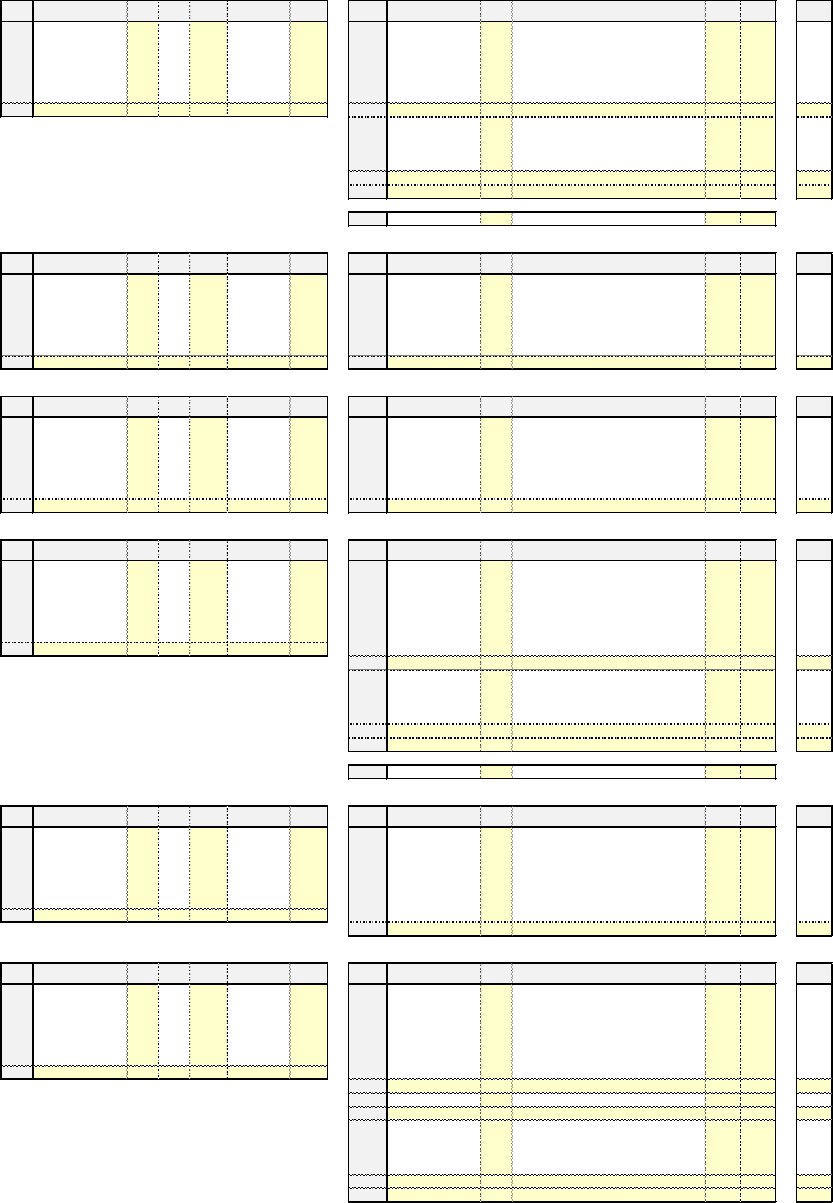
Handbook on Supply and Use Tables and Input-Output Tables with Extensions and Applications
354
Table A11.2: Price indices for supply and use tables 2011
AGR MMC SER DP IMP SUPbp TTM TLS SUPpp AGR MMC SER TIC FCH FCN FCG GFCF INV E XP TOTfin TOTpp Check
AGR 102.0 104.1 102.0 106.9 103.8 97.5 107.6 102.5 AGR 105.8 109.9 98.7 108.2 100.4 94.7 568.8 97.7 98.0 102.4 0.0
MAN 107.5 108.0 100.5 107.2 108.0 107.6 101.1 103.2 106.4 MAN 114.1 110.4 105.0 109.2 102.1 99.5 99.6 85.7 106.7 104.9 106.2 0.2
CON 103.4 100.5 100.5 100.5 101.6 100.5 100.1 100.4 CON 101.4 100.5 101.8 101.0 97.4 97.1 100.0 102.0 100.0 100.5 0.0
TTC 101.1 99.2 100.3 100.2 110.7 102.4 100.8 101.4 103.4 TTC 100.9 100.1 100.8 100.7 102.2 108.0 106.2 104.0 -0.5
FBS 102.9 100.9 100.4 100.4 101.0 100.5 93.6 100.3 FBS 101.4 100.7 100.4 100.5 101.7 101.8 99.0 100.1 100.3 0.0
OSE 100.2 101.0 103.4 101.1 99.1 110.2 101.2 OSE 102.4 101.7 104.3 103.9 102.7 103.8 101.7 99.5 101.8 100.9 101.2 0.0
TOT 102.2 105.8 100.5 102.4 107.3 103.7 101.6 103.7 TIC 109.3 107.5 101.7 104.5 102.1 103.3 100.2 99.1 83.0 105.7 103.2 103.6 -0.3
OTLS 98.0 201.1 269.9 48.3 48.3
COE 102.7 101.9 101.5 101.6 101.6
CFC 99.1 100.6 98.4 98.8 98.8
NOS 80.9 103.2 96.2 97.7 97.7
GVA 91.1 102.2 99.7 100.1 100.1
TOT 102.2 105.8 100.5 102.4 102.1 103.3 100.2 99.1 83.0 105.7 103.2
Check
AGR MMC SER DP IMP SUPbp TTM TLS SUPpp AGR MMC SER TIC FCH FCN FCG GFCF INV E XP TOTfin TOTpp Check
AGR 107.6 AGR 92.3 612.5 91.4 230.0 100.8 96.2 99.8 107.6
MAN 103.2 MAN 103.7 107.3 103.9 104.6 101.7 98.7 93.8 -100.0 104.4 101.3 101.9 1.3
CON 100.1 CON 102.2 102.1 90.7 95.1 99.6 100.0 99.4 100.1
TTC 101.4 TTC 99.4 103.3 102.4 101.4
FBS 93.6 FBS 123.1 100.0 102.0 102.1 105.7 103.8 44.4 86.4 93.3 0.3
OSE 110.2 OSE 241.7 109.2 101.1 108.5 110.2
TOT 101.6 TOT 105.1 110.1 103.1 103.8 102.5 102.3 92.5 -100.0 105.0 99.8 100.7 0.8
AGR MMC SER DP IMP SUPbp TTM TLS SUPpp AGR MMC SER TIC FCH FCN FCG GFCF INV E XP TOTfin TOTpp Check
AGR 97.5 AGR 90.4 96.7 100.7 96.3 104.9 85.7 100.0 94.0 97.9 97.5
MAN 101.1 MAN 113.7 102.6 102.3 102.8 97.8 97.9 97.5 93.5 99.5 98.5 99.6 1.5
CON CON
TTC 100.8 TTC 105.0 102.1 102.2 102.3 98.3 97.9 97.5 93.8 98.8 98.4 99.4 1.4
FBS FBS
OSE 99.1 OSE 97.6 104.2 99.1 99.1
TOT TOT
AGR MMC SER DP IMP SUPbp TTM TLS SUPpp AGR MMC SER TIC FCH FCN FCG GFCF INV E XP TOTfin TOTpp Check
AGR 102.0 104.1 102.0 106.9 103.8 AGR 107.2 111.2 98.1 109.5 94.9 95.6 725.0 98.9 98.0 103.8 0.0
MAN 107.5 108.0 100.5 107.2 108.0 107.6 MAN 114.4 111.4 105.6 110.2 105.5 100.5 100.2 85.7 107.5 106.3 107.6 -0.1
CON 103.4 100.5 100.5 100.5 101.6 100.5 CON 101.4 100.5 101.7 101.0 98.3 97.4 100.0 102.0 100.1 100.5 0.0
TTC 101.1 99.2 100.3 100.2 110.7 102.4 TTC 103.8 101.5 101.0 101.2 99.5 98.5 97.0 93.7 105.0 102.8 102.2 0.2
FBS 102.9 100.9 100.4 100.4 101.0 100.5 FBS 101.2 100.7 100.4 100.5 101.7 101.7 100.6 99.0 100.6 100.5 0.0
OSE 100.2 101.0 103.4 101.1 OSE 102.4 101.8 104.1 103.7 102.4 103.8 102.5 99.5 101.5 100.8 101.1 0.0
TOT 102.2 105.8 100.5 102.4 107.3 103.7 TLS 105.1 110.1 103.1 103.8 102.5 102.3 92.5 -100.0 105.0 99.8 100.7
TIC 109.3 107.5 101.7 104.5 102.1 103.3 100.2 99.1 83.0 105.7 103.2 103.6 0.1
OTLS 98.0 201.1 269.9 48.3 48.3
COE 102.7 101.9 101.5 101.6 101.6
CFC 99.1 100.6 98.4 98.8 98.8
NOS 80.9 103.2 96.2 97.7 97.7
GVA 91.1 102.2 99.7 100.1 100.1
TOT 102.2 105.8 100.5 102.4 102.1 103.3 100.2 99.1 83.0 105.7 103.2
Check
AGR MMC SER DP IMP SUPbp TTM TLS SUPpp AGR MMC SER TIC FCH FCN FCG GFCF INV E XP TOTfin TOTpp Check
AGR 106.9 AGR 113.0 114.5 98.0 113.2 100.1 100.0 207.1 102.1 101.4 106.9
MAN 108.0 MAN 112.6 114.4 107.2 113.1 102.0 99.6 99.5 -311.5 89.4 92.1 99.9 8.1
CON 101.6 CON 100.0 101.0 102.0 101.4 101.8 101.8 101.6
TTC 110.7 TTC 100.0 100.5 101.2 115.2 113.9 110.7 -0.1
FBS 101.0 FBS 97.0 101.4 100.4 100.8 106.7 101.6 101.0
OSE 103.4 OSE 100.0 100.8 101.4 101.4 104.2 99.0 97.1 104.1 103.4
TOT 107.3 TLS
TIC 110.7 112.3 102.8 108.9 102.6 99.6 99.4 -100.8 96.5 97.6 102.0 5.3
AGR MMC SER DP IMP SUPbp TTM TLS SUPpp AGR MMC SER TIC FCH FCN FCG GFCF INV E XP TOTfin TOTpp Check
AGR 102.0 104.1 102.0 AGR 106.2 109.0 98.2 107.6 90.0 94.6 -181.3 97.0 95.9 102.0 0.0
MAN 107.5 108.0 100.5 107.2 MAN 114.7 107.9 104.5 107.5 108.4 100.8 100.7 98.0 120.7 116.7 113.9 -6.7
CON 103.4 100.5 100.5 100.5 CON 101.4 100.5 101.7 101.0 98.3 97.4 100.0 102.0 100.0 100.5 0.0
TTC 101.1
99.2 100.3 100.2 TTC 103.9 101.5 100.9 101.2 99.5 98.5 97.2 93.5 99.2 99.2 99.9 0.3
FBS 102.9 100.9 100.4 100.4 FBS 101.8 100.4 100.4 100.4 101.7 101.7 100.5 98.0 100.5 100.4 0.0
OSE 100.2 101.0 OSE 102.5 101.9 104.7 104.2 101.9 103.8 102.5 100.0 101.5 100.7 101.0 0.0
TOT 102.2 105.8 100.5 102.4 TLS 105.1 110.1 103.1 103.8 102.5 102.3 92.5 -100.0 105.0 99.8 100.7
TIC 109.1 104.4 101.4 102.8 102.0 103.3 100.2 99.0 96.1 111.5 104.9 104.2 -6.4
IMP 110.7 112.3 102.8 108.9 102.6 99.6 99.4 -100.8 96.5 97.6 102.0
TOT 109.3 107.5 101.7 104.5 102.1 103.3 100.2 99.1 83.0 105.7 103.2 103.6 -6.4
OTLS 98.0 201.1 269.9 48.3 48.3
COE 102.7 101.9 101.5 101.6 101.6
CFC 99.1 100.6 98.4 98.8 98.8
NOS 80.9 103.2 96.2 97.7 97.7
GVA 91.1 102.2 99.7 100.1 100.1
TOT 102.2 105.8 100.5 102.4 102.1 103.3 100.2 99.1 83.0 105.7 103.2
Domestic Use Table at basic prices
Supply Table at basic prices, transf. to purchasers' prices
Taxes less subsidies on products
Trade and transport margins
Supply Table at basic prices
Imports cif
Supply Table for domestic output at basic prices
Use Table at purchasers' prices
Use Table for taxes less subsidies on products
Use Table for trade and transport margins
Use Table at basic prices
Imports Use Table

Handbook on Supply and Use Tables and Input-Output Tables with Extensions and Applications
355
Table A11.3: Supply and use tables 2011 at previous years' prices
AGR MMC
SER
DP IMP
SUPbp
TTM
TLS
SUPpp
AGR MMC
SER TIC
FCH
FCN FCG
GFCF
INV E XP TOTfi n TOTpp Check
AGR 25.5 0.1 0.0 25.7 14.4 40.1 11.2 0.5 51.8 AGR 5.2 15.8 1.6 22.6 5.9 0.2 0.0 22.9 29.0 51.5 0.2
MAN 1.2 295.0 35.6 331.7 311.9 643.7 111.7 38.2 793.6 MAN 8.9 183.1 62.3 254.4 120.3 9.2 51.7 1.6 358.9 541.7 796.1 -2.5
CON 0.1 87.6 4.5 92.2 1.5 93.7 8.3 102.0 CON 0.3 26.1 19.4 45.8 0.5 0.6 53.7 2.1 56.8 102.6 -0.7
TTC 0.5 15.2 231.0 246.7 66.4 313.1 -123.0 3.0 193.0 TTC 0.6 10.8 65.6 77.0 21.0 0.9 0.5 6.9 0.0 85.5 114.7 191.7 1.3
FBS 0.5 8.0 280.8 289.2 54.7 343.9 9.7 353.7 FBS 2.0 43.2 161.1 206.3 76.6 0.0 3.5 17.6 50.0 147.7 354.0 -0.3
OSE 0.3 2.5 220.7 223.5 16.1 239.6 0.1 2.7 242.4 OSE 0.2 3.5 21.2 24.9 53.2 4.4 153.1 1.1 0.2 5.0 217.1 242.0 0.4
TOT 28.1 408.4 772.5 1209.0 465.0 1674.0 0.0 62.4 1736.4 TIC 17.2 282.5 331.3 630.9 277.5 5.3 166.8 131.3 1.8 524.3 1107.0 1737.9 -1.5
OTLS -0.7 0.1 0.1 -0.5 -0.5
COE 2.6 59.8 250.6 313.0 313.0
CFC 3.7 20.4 84.3 108.4 108.4
NOS 5.3 45.7 106.3 157.3 157.3
GVA 10.9 126.0 441.2 578.1 578.1
TOT 28.1 408.4 772.5 1209.0 277.5 5.3 166.8 131.3 1.8 524.3 1107.0
Check
AGR MMC SER DP IMP SUPbp TTM TLS SUPpp AGR MMC SER TIC FCH FCN FCG GFCF INV E XP TOTfin TOTpp Check
AGR 0.5 AGR 0.0 0.0 0.0 0.0 0.4 0.1 0.5 0.5
MAN 38.2 MAN 0.2 1.6 6.2 8.0 26.4 0.4 2.3 0.0 1.6 30.7 38.7 -0.5
CON 8.3 CON 0.0 2.0 2.0 0.1 0.1 6.1 0.0 6.3 8.3
TTC 3.0 TTC 0.0 -0.1 1.1 1.0 1.7 -0.1 0.5 -0.1 2.0 3.0
FBS 9.7 FBS 0.0 0.0 4.3 4.3 1.5 0.1 3.9 0.0 5.5 9.7
OSE 2.7 OSE 0.0 0.0 0.0 2.1 -0.4 0.7 0.3 2.7 2.7
TOT 62.4 TOT 0.2 1.5 13.6 15.3 32.1 0.1 13.5 0.0 1.9 47.6 62.9 -0.5
AGR MMC SER DP IMP SUPbp TTM TLS SUPpp AGR MMC SER TIC FCH FCN FCG GFCF INV E XP TOTfin TOTpp Check
AGR 11.2 AGR 0.4 1.7 0.4 2.6 3.1 0.0 0.0 5.6 8.6 11.2
MAN 111.7 MAN 0.8 20.0 9.0 29.8 39.9 3.2 5.2 -0.1 34.7 82.9 112.7 -1.0
CON CON
TTC -123.0 TTC -1.2 -21.7 -9.4 -32.3 -43.1 -3.2 -5.2
0.1 -40.2 -91.7 -124.0 1.0
FBS FBS
OSE 0.1 OSE 0.1 0.0 0.1 0.1
TOT 0.0 TOT 0.0 0.0 0.0 0.0 0.0 0.0 0.0 0.0 0.0
AGR MMC SER DP IMP SUPbp TTM TLS SUPpp AGR MMC SER TIC FCH FCN FCG GFCF INV E XP TOTfin TOTpp Check
AGR 25.5 0.1 0.0 25.7 14.4 40.1 AGR 4.8 14.1 1.1 20.0 2.5 0.1 0.0 17.2 19.9 39.8 0.2
MAN 1.2 295.0 35.6 331.7 311.9 643.7 MAN 7.9 161.6 47.1 216.6 53.9 5.6 44.2 1.7 322.6 428.0 644.7 -1.0
CON 0.1 87.6 4.5 92.2 1.5 93.7 CON 0.3 26.1 17.4 43.8 0.4 0.5 47.6 2.1 50.6 94.4 -0.7
TTC 0.5 15.2 231.0 246.7 66.4 313.1 TTC 1.8 32.5 74.0 108.3 62.4 0.9 3.8 11.7 -0.1 125.8 204.4 312.8 0.3
FBS 0.5 8.0 280.8 289.2 54.7 343.9 FBS 2.0 43.2 156.8 202.0 75.1 0.0 3.4 13.7 50.0 142.2 344.2 -0.3
OSE 0.3 2.5 220.7 223.5 16.1 239.6 OSE 0.2 3.5 21.2 24.9 51.0 4.4 153.5 0.4 0.2 4.7 214.3 239.2 0.4
TOT 28.1 408.4 772.5 1209.0 465.0 1674.0 TLS 0.2 1.5 13.6 15.3 32.1 0.1 13.5 0.0 1.9 47.6 62.9
TIC 17.2 282.5 331.3 630.9 277.5 5.3 166.8 131.3 1.8 524.3 1107.0 1737.9 -1.0
OTLS -0.7 0.1 0.1 -0.5 -0.5
COE 2.6 59.8 250.6 313.0 313.0
CFC 3.7 20.4 84.3 108.4 108.4
NOS 5.3 45.7 106.3 157.3 157.3
GVA 10.9 126.0 441.2 578.1 578.1
TOT 28.1 408.4 772.5 1209.0 277.5 5.3 166.8 131.3 1.8 524.3 1107.0
Check
AGR MMC SER DP IMP SUPbp TTM TLS SUPpp AGR MMC SER TIC FCH FCN FCG GFCF INV E XP TOTfin TOTpp Check
AGR 14.4 AGR 0.7 5.6 0.5 6.8 1.2 0.0 0.0 6.4 7.6 14.4
MAN 311.9 MAN 1.1 85.6 19.5 106.2 24.0 1.6 19.3 0.1 135.7 180.7 286.9 25.0
CON 1.5 CON 0.0 0.5 0.3 0.9 0.7 0.7 1.5
TTC 66.4 TTC 0.0 2.7 13.9 16.6 0.7 2.8 0.0 45.8 49.3 65.9 0.5
FBS 54.7 FBS 0.2 13.8 24.4 38.5 0.2 2.1 13.9 16.2 54.7
OSE 16.1 OSE 0.0 0.5 3.9 4.4 11.6 0.0 0.1 0.0 11.7 16.1
TOT 465.0 TLS
TIC 2.1 108.7 62.5 173.3 37.7 1.6 24.9 0.1 201.8 266.2 439.5 25.5
AGR MMC SER DP IMP SUPbp TTM TLS SUPpp AGR MMC SER TIC FCH FCN FCG GFCF INV E XP TOTfin TOTpp Check
AGR 25.5 0.1 0.0 25.7 AGR 4.1 8.5 0.6 13.2 1.3 0.1 0.0 10.8 12.2 25.5 0.2
MAN 1.2
295.0 35.6 331.7 MAN 6.8 75.9 27.7 110.4 29.9 3.9 24.9 1.7 186.9 247.3 357.7 -26.0
CON 0.1 87.6 4.5 92.2 CON 0.3 25.6 17.1 43.0 0.4 0.5 46.9 2.1 49.9 92.8 -0.7
TRA 0.5 15.2 231.0 246.7 TTC 1.7 29.9 60.2 91.8 61.7 0.9 3.8 8.9 -0.1 80.0 155.1 246.9 -0.2
TRN 0.5 8.0 280.8 289.2 FBS 1.8 29.4 132.4 163.5 74.9 0.0 3.4 11.6 36.1 126.0 289.5 -0.3
COM 0.3 2.5 220.7 223.5 OSE 0.2 3.0 17.3 20.5 39.5 4.4 153.5 0.4 0.1 4.7 202.6 223.1 0.4
TOT 28.1 408.4 772.5 1209.0 TLS 0.2 1.5 13.6 15.3 32.1 0.1 13.5 0.0 1.9 47.6 62.9
TIC 15.1 173.7 268.8 457.6 239.8 5.3 165.2 106.4 1.7 322.5 840.8 1298.4 -26.5
IMP 2.1 108.7 62.5 173.3 37.7 1.6 24.9 0.1 201.8 266.2 439.5
TOT 17.2 282.5 331.3 630.9 277.5 5.3 166.8 131.3 1.8 524.3 1107.0 1737.9 -26.5
OTLS -0.7 0.1 0.1 -0.5 -0.5
COE 2.6 59.8 250.6 313.0 313.0
CFC 3.7 20.4 84.3 108.4 108.4
NOS 5.3 45.7 106.3 157.3 157.3
GVA 10.9 126.0 441.2 578.1 578.1
TOT 28.1 408.4 772.5 1209.0 277.5 5.3 166.8 131.3 1.8 524.3 1107.0
Check
Supply Table at basic prices
Use Table at basic prices
Imp o rts C IF
Imports Use Table
Supply Table for domestic output at basic prices
Domestic Use Table at basic prices
Supply Table at basic prices, transf. to purchasers' prices
Use Table at purchasers' prices
Taxes less subsidies on products
Use Table for taxes less subsidies on products
Trade and transport margins
Use Table for trade and transport margins

Handbook on Supply and Use Tables and Input-Output Tables with Extensions and Applications
356
Table A11.4: Volume indices for supply and use tables 2011
AGR
MMC SER DP IMP SUPbp TTM TLS SUPpp AGR MMC SER TIC FCH FCN FCG GFCF INV E XP TOTfin TOTpp Check
AGR 100.8 96.1 87.8 100.8 103.5 101.8 103.6 111.9 102.2 AGR 102.0 103.4 96.5 102.6 101.5 84.8 -9.1 102.0 101.1 101.8 0.5
MAN 95.4 104.4 99.4 103.8 103.3 103.6 102.7 97.4 103.1 MAN 99.5 105.6 98.5 103.6 99.4 102.8 112.5 43.1 104.3 103.4 103.5 -0.3
CON 127.1 103.2 95.6 102.8 101.2 102.8 98.2 102.4 CON 100.7 110.7 100.2 105.9 103.3 96.0 101.3 91.6 100.9 103.1 -0.7
TTC 92.6 98.9 103.8 103.4 101.9 103.1 102.8 95.1 103.2 TTC 99.1 100.0 101.3 101.1 99.7 104.5 103.4 102.5 0.7
FBS 99.6 102.2 102.1 102.1 107.4 102.9 98.2 102.8 FBS 98.9 104.7 103.0 103.3 100.5 96.2 106.2 102.2 102.9 -0.1
OSE 95.2 99.1 100.5 100.5 98.3 100.3 94.6 101.9 100.4 OSE 99.4 101.8 101.4 101.5 101.0 99.8 98.2 72.6 103.1 100.0 100.2 0.2
TOT 100.4 103.8 102.0 102.6 103.4 102.8 104.2 97.8 102.6 TIC 100.2 105.5 101.5 103.2 100.1 99.8 99.8 105.3 42.7 104.3 102.4 102.7 0.2
OTLS 137.2 -84.9 -30.6 55.5 55.5
COE 100.1 100.0 101.0 100.8 100.8
CFC 101.6 100.9 101.4 101.3 101.3
NOS 104.4 99.9 105.9 104.0 104.0
GVA 100.8 100.2 102.3 101.8 101.8
TOT 100.4 103.8 102.0 102.6 100.1 99.8 99.8 105.3 42.7 104.3 102.4
Check
AGR MMC SER DP IMP SUPbp TTM TLS SUPpp AGR MMC SER TIC FCH FCN FCG GFCF INV E XP TOTfin TOTpp Check
AGR 111.9 AGR 92.9 -40.0 134.6 -375.0 101.4 110.5 103.3 111.9
MAN 97.4 MAN 94.3 97.2 97.6 97.5 98.2 100.8 105.1 -100.0 104.0 99.0 98.7 -1.3
CON 98.2 CON 98.1 98.1 105.9 96.5 98.2 100.0 98.2 98.2
TTC 95.1 TTC 92.2 98.2 96.7 95.1
FBS 98.2 FBS 130.0 -14.3 100.4 100.7 102.9 89.0 225.0 96.3 98.2
OSE 101.9 OSE 240.0 101.0 101.1 101.1 101.9
TOT 97.8 TOT 96.4 99.7 98.3 98.4 98.7 79.8 98.2 -100.0 103.5 98.7 98.6 -0.8
AGR MMC SER DP IMP SUPbp TTM TLS SUPpp AGR MMC SER TIC FCH FCN FCG GFCF INV E XP TOTfin TOTpp Check
AGR 103.6 AGR 101.4 104.6 95.9 102.5 101.7 82.4 -50.0 105.4 103.9 103.6
MAN 102.7 MAN 97.9 107.5 97.8 104.1 100.7 101.5 118.6 -183.3 105.2 103.4 103.6 -0.9
CON CON
TTC 102.8 TTC 99.2 107.3 97.7 104.0 100.8 101.5 118.5 -162.0 105.2 103.5 103.6 -0.8
FBS FBS
OSE 94.6 OSE 95.3 92.3 94.6 94.6
TOT TOT
AGR MMC SER
DP IMP SUPbp TTM TLS SUPpp AGR MMC SER TIC FCH FCN FCG GFCF INV E XP TOTfin TOTpp Check
AGR 100.8 96.1 100.8 103.5 101.8 AGR 102.1 103.1 95.9 102.4 101.3 85.1 -7.1 100.9 99.9 101.1 0.6
MAN 95.4 104.4 99.4 103.8 103.3 103.6 MAN 99.8 105.5 98.7 103.7 99.0 103.7 112.3 45.7 104.2 103.8 103.7 -0.2
CON 127.1 103.2 95.6 102.8 101.2 102.8 CON 100.7 110.7 100.4 106.3 103.0 96.0 101.7 91.6 101.2 103.5 -0.7
TTC 92.6 98.9 103.8 103.4 101.9 103.1 TTC 99.1 104.7 101.0 102.1 100.5 101.0 109.7 -102.6 104.7 103.5 103.0 0.1
FBS 99.6 102.2 102.1 102.1 107.4 102.9 FBS 98.7 104.7 103.1 103.4 100.5 96.4 102.0 106.2 102.5 103.0 -0.1
OSE 99.1 100.5 98.3 100.3 OSE 99.4 101.6 101.4 101.4 101.0 99.8 93.7 72.6 103.2 100.0 100.2 0.2
TOT 100.4 103.8 102.0 102.6 103.4 102.8 TLS 96.4 99.7 98.3 98.4 98.7 79.8 98.2 -100.0 103.5 98.7 98.6
TIC 100.2 105.5 101.5 103.2 100.1 99.8 99.8 105.3 42.7 104.3 102.4 102.7 -0.1
OTLS 137.2 -84.9 -30.6 55.5 55.5
COE 100.1 100.0 101.0 100.8 100.8
CFC 101.6 100.9 101.4 101.3 101.3
NOS 104.4 99.9 105.9 104.0 104.0
GVA 100.8 100.2 102.3 101.8 101.8
TOT 100.4 103.8 102.0 102.6 100.1 99.8 99.8 105.3 42.7 104.3 102.4
Check
AGR MMC SER DP IMP SUPbp TTM TLS SUPpp AGR MMC SER TIC FCH FCN FCG GFCF INV E XP TOTfin TOTpp Check
AGR 103.5 AGR 100.9 106.3 88.2 104.2 105.0 78.8 -32.2 104.5 102.9 103.5
MAN 103.3 MAN 104.1 106.6 99.7 105.2 100.4 92.0 117.4 3.1 86.4 90.0 95.1 8.3
CON 101.2 CON 100.0 110.6 96.6 104.5 97.4 97.4 101.2
TTC 101.9 TTC 102.3 99.0 100.2 101.7 101.4 101.1 0.8
FBS 107.4 FBS 98.8 103.5 107.7 106.1 92.1 110.8 107.4
OSE 98.3 OSE 85.7 104.5 101.8 102.1 97.6 57.8 97.2 97.0 98.3
TOT 103.4 TLS
TIC 102.3 105.9 102.9 104.8 99.7 92.2 114.7 6.3 91.3 93.6 97.7 5.7
AGR MMC SER DP IMP SUPbp TTM TLS SUPpp AGR MMC SER TIC FCH FCN FCG GFCF INV E XP TOTfin TOTpp Check
AGR 100.8 96.1 100.8 AGR 102.3 101.0 103.0 101.5 98.0 86.7 19.8 98.9 98.1 99.9 0.9
MAN 95.4 104.4 99.4 103.8 MAN 99.1 104.3 98.0 102.3 98.0 109.4 108.6 79.6 122.5 116.8 111.9 -8.1
CON 127.1 103.2 95.6 102.8 CON 100.7 110.7 100.5 106.3 103.0 96.0 101.8 91.6 101.3 103.5 -0.8
TTC 92.6 98.9 103.8 103.4 TTC 99.0 105.3 101.1 102.4
100.5 101.0 114.6 -110.0 106.6 104.2 103.5 -0.1
FBS 99.6 102.2 102.1 102.1 FBS 98.7 105.3 102.3 102.8 100.5 96.4 98.3 105.3 101.5 102.2 -0.1
OSE 99.1 100.5 OSE 100.0 101.2 101.3 101.2 102.1 99.8 93.7 95.5 103.2 100.2 100.3 0.2
TOT 100.4 103.8 102.0 102.6 TLS 96.4 99.7 98.3 98.4 98.7 79.8 98.2 -100.0 103.5 98.7 98.6
TIC 99.9 105.3 101.2 102.7 100.2 99.8 99.8 103.3 72.5 114.6 105.5 104.5 -8.0
IMP 102.3 105.9 102.9 104.8 99.7 92.2 114.7 6.3 91.3 93.6 97.7
TOT 100.2 105.5 101.5 103.2 100.1 99.8 99.8 105.3 42.7 104.3 102.4 102.7 -8.0
OTLS 137.2 -84.9 -30.6 55.5 55.5
COE 100.1 100.0 101.0 100.8 100.8
CFC 101.6 100.9 101.4 101.3 101.3
NOS 104.4 99.9 105.9 104.0 104.0
GVA 100.8 100.2 102.3 101.8 101.8
TOT 100.4 103.8 102.0 102.6 100.1 99.8 99.8 105.3 42.7 104.3 102.4
Supply Table for domestic output at basic prices
Domestic Use Table at basic prices
Trade and transport margins
Use Table for trade and transport margins
Supply Table at basic prices
Use Table at basic prices
Imp o rts C IF
Imports Use Table
Supply Table at basic prices, transf. to purchasers' prices
Use Table at purchasers' prices
Taxes less subsidies on products
Use Table for taxes less subsidies on products

Handbook on Supply and Use Tables and Input-Output Tables with Extensions and Applications
357
Table A11.5: Supply and use tables 2010 in current prices
AGR MMC SER DP IMP SUPbp TTM TLS SUPpp AGR MMC SER TIC FCH FCN FCG GFCF INV E XP TOTfin TOTpp Check
AGR 25.3 0.2 0.0 25.5 13.9 39.4 10.8 0.4 50.6 AGR 5.1 15.3 1.6 22.0 5.8 0.2 0.2 22.5 28.6 50.6
MAN 1.2 282.6 35.8 319.6 301.8 621.4 108.8 39.2 769.4 MAN 8.9 173.4 63.3 245.6 121.0 8.9 46.0 3.8 344.1 523.7 769.4
CON 0.1 84.9 4.7 89.7 1.5 91.2 8.4 99.6 CON 0.3 23.6 19.4 43.2 0.5 0.6 53.0 2.2 56.4 99.6
TTC 0.6 15.4 222.6 238.5 65.1 303.6 -119.7 3.1 187.1 TTC 0.6 10.8 64.8 76.1 21.0 0.9 0.5 6.7 0.0 81.8 110.9 187.1
FBS 0.5 7.8 275.0 283.3 50.9 334.2 9.9 344.1 FBS 2.1 41.2 156.3 199.6 76.2 0.0 3.7 17.5 47.1 144.5 344.1
OSE 0.3 2.5 219.6 222.4 16.4 238.8 0.1 2.7 241.6 OSE 0.2 3.4 20.9 24.5 52.7 4.5 153.6 1.2 0.3 4.9 217.0 241.6
TOT 28.0 393.3 757.6 1178.9 449.7 1628.6 0.0 63.8 1692.3 TIC 17.1 267.7 326.4 611.2 277.2 5.3 167.2 124.6 4.3 502.5 1081.2 1692.3
OTLS -0.5 -0.1 -0.3 -1.0 -1.0
COE 2.6 59.8 248.1 310.5 310.5
CFC 3.7 20.2 83.1 107.0 107.0
NOS 5.1 45.8 100.4 151.3 151.3
GVA 10.8 125.7 431.2 567.8 567.8
TOT 28.0 393.3 757.6 1178.9 277.2 5.3 167.2 124.6 4.3 502.5 1081.2
Check
AGR MMC SER DP IMP SUPbp TTM TLS SUPpp AGR MMC SER TIC FCH FCN FCG GFCF INV E XP TOTfin TOTpp Check
AGR 0.4 AGR 0.0 0.0 0.0 0.0 0.4 0.1 0.5 0.4
MAN 39.2 MAN 0.2 1.6 6.3 8.2 26.9 0.4 2.2 0.0 1.6 31.0 39.2
CON 8.4 CON 0.0 2.0 2.0 0.1 0.1 6.3 0.0 6.4 8.4
TTC 3.1 TTC 0.0 -0.1 1.1 1.1 1.7 -0.1 0.5 -0.1 2.0 3.1
FBS 9.9 FBS 0.0 0.0 4.3 4.3 1.5 0.1 4.1 0.0 5.7 9.9
OSE 2.7 OSE 0.0 0.0 0.0 2.1 -0.4 0.7 0.3 2.7 2.7
TOT 63.8 TOT 0.2 1.5 13.8 15.5 32.5 0.1 13.8 0.0 1.8 48.2 63.8
AGR MMC SER DP IMP SUPbp TTM TLS SUPpp AGR MMC SER TIC FCH FCN FCG GFCF INV E XP TOTfin TOTpp Check
AGR 10.8 AGR 0.4 1.6 0.4 2.5 3.0 0.0 0.0 5.3 8.3 10.8
MAN 108.8 MAN 0.8 18.6 9.2 28.6 39.6 3.2 4.4 0.0 32.9 80.2 108.8
CON CON
TTC -119.7 TTC -1.2 -20.2 -9.7 -31.1 -42.7 -3.2 -4.4 -0.1 -38.2 -88.6 -119.7
FBS FBS
OSE 0.1 OSE
0.1 0.0 0.1 0.1
TOT 0.0 TOT 0.0 0.0 0.0 0.0 0.0 0.0
AGR MMC SER DP IMP SUPbp TTM TLS SUPpp AGR MMC SER TIC FCH FCN FCG GFCF INV E XP TOTfin TOTpp Check
AGR 25.3 0.2 0.0 25.5 13.9 39.4 AGR 4.7 13.7 1.2 19.5 2.5 0.2 0.2 17.1 19.9 39.4
MAN 1.2 282.6 35.8 319.6 301.8 621.4 MAN 7.9 153.2 47.8 208.9 54.5 5.4 39.4 3.8 309.6 412.5 621.4
CON 0.1 84.9 4.7 89.7 1.5 91.2 CON 0.3 23.6 17.4 41.2 0.4 0.5 46.8 2.2 50.0 91.2
TTC 0.6 15.4 222.6 238.5 65.1 303.6 TTC 1.8 31.1 73.3 106.2 62.1 0.9 3.7 10.7 0.1 120.1 197.5 303.6
FBS 0.5 7.8 275.0 283.3 50.9 334.2 FBS 2.1 41.2 152.1 195.4 74.8 0.0 3.5 13.4 47.1 138.8 334.2
OSE 0.3 2.5 219.6 222.4 16.4 238.8 OSE 0.2 3.4 20.9 24.5 50.5 4.5 154.0 0.5 0.3 4.6 214.3 238.8
TOT 28.0 393.3 757.6 1178.9 449.7 1628.6 TLS 0.2 1.5 13.8 15.5 32.5 0.1 13.8 0.0 1.8 48.2 63.8
TIC 17.1 267.7 326.4 611.2 277.2 5.3 167.2 124.6 4.3 502.5 1081.2 1692.3
OTLS -0.5 -0.1 -0.3 -1.0 -1.0
COE 2.6 59.8 248.1 310.5 310.5
CFC 3.7 20.2 83.1 107.0 107.0
NOS 5.1 45.8 100.4 151.3 151.3
GVA 10.8 125.7 431.2 567.8 567.8
TOT 28.0 393.3 757.6 1178.9 277.2 5.3 167.2 124.6 4.3 502.5 1081.2
Check
AGR MMC SER DP IMP SUPbp TTM TLS SUPpp AGR MMC SER TIC FCH FCN FCG GFCF INV E XP TOTfin TOTpp Check
AGR 13.9 AGR 0.7 5.3 0.6 6.5 1.2 0.0 0.1 6.1 7.4 13.9
MAN 301.8 MAN 1.1 80.4 19.5 101.0 23.9 1.8 16.4 1.7 157.1 200.9 301.8
CON 1.5 CON 0.0 0.5 0.4 0.8 0.7 0.7 1.5
TTC 65.1 TTC 0.0 2.7 13.8 16.6 0.7 2.9 0.0 45.0 48.6 65.1
FBS 50.9 FBS 0.2 13.3 22.7 36.3 0.2 1.7 12.8 14.6 50.9
OSE 16.4 OSE 0.0 0.5 3.8 4.3 11.8 0.2 0.0 12.1 16.4
TOT 449.7 TLS
TIC 2.0 102.6 60.8 165.4 37.8 1.8 21.7 1.9 221.0 284.2 449.7
AGR MMC SER DP IMP SUPbp TTM TLS SUPpp AGR MMC SER TIC FCH FCN FCG GFCF INV E XP TOTfin TOTpp Check
AGR 25.3 0.2 0.0 25.5 AGR 4.0 8.4 0.6 13.0 1.3 0.1 0.1 10.9 12.5 25.5
MAN 1.2 282.6 35.8 319.6 MAN 6.8 72.8 28.2 107.9 30.6 3.6 22.9 2.1 152.5 211.7 319.6
CON 0.1 84.9 4.7 89.7 CON 0.3 23.1 17.0 40.4
0.4 0.5 46.1 2.2 49.3 89.7
TTC 0.6 15.4 222.6 238.5 TTC 1.7 28.4 59.5 89.6 61.4 0.9 3.7 7.8 0.1 75.1 148.9 238.5
FBS 0.5 7.8 275.0 283.3 FBS 1.8 27.9 129.4 159.1 74.5 0.0 3.5 11.8 34.3 124.2 283.3
OSE 0.3 2.5 219.6 222.4 OSE 0.2 2.9 17.1 20.2 38.7 4.5 154.0 0.5 0.1 4.5 202.2 222.4
TOT 28.0 393.3 757.6 1178.9 TLS 0.2 1.5 13.8 15.5 32.5 0.1 13.8 0.0 1.8 48.2 63.8
TIC 15.1 165.0 265.6 445.7 239.4 5.3 165.5 102.9 2.4 281.5 796.9 1242.7
IMP 2.0 102.6 60.8 165.4 37.8 1.8 21.7 1.9 221.0 284.2 449.7
TOT 17.1 267.7 326.4 611.2 277.2 5.3 167.2 124.6 4.3 502.5 1081.2 1692.3
OTLS -0.5 -0.1 -0.3 -1.0 -1.0
COE 2.6 59.8 248.1 310.5 310.5
CFC 3.7 20.2 83.1 107.0 107.0
NOS 5.1 45.8 100.4 151.3 151.3
GVA 10.8 125.7 431.2 567.8 567.8
TOT 28.0 393.3 757.6 1178.9 277.2 5.3 167.2 124.6 4.3 502.5 1081.2
Check
Supply Table at basic prices
Use Table at basic prices
Imp o rts C IF
Imports Use Table
Supply Table for domestic output at basic prices
Domestic Use Table at basic prices
Supply Table at basic prices, transf. to purchasers' prices
Use Table at purchasers' prices
Taxes less subsidies on products
Use Table for taxes less subsidies on products
Trade and transport margins
Use Table for trade and transport margins

Handbook on Supply and Use Tables and Input-Output Tables with Extensions and Applications
358
2. Balanced supply and use tables (tables A11.6–A11.10)
Table A11.6: Supply and use tables 2011 in current prices
AGR MMC SER DP IMP SUPbp TTM TLS SUPpp AGR MMC SER TIC FCH FCN FCG GFCF INV E XP TOTfin TOTpp Check
AGR 25.8 0.2 0.0 26.0 15.4 41.3 10.9 0.5 52.8 AGR 5.5 17.4 1.5 24.4 5.9 0.1 -0.1 22.4 28.4 52.8
MAN 1.3 318.5 35.7 355.5 336.8 692.3 113.0 39.4 844.7 MAN 10.1 202.1 65.4 277.7 122.8 9.1 51.5 1.4 382.1 567.0 844.7
CON 0.1 89.0 4.5 93.6 1.6 95.1 8.3 103.4 CON 0.3 26.2 19.8 46.3 0.5 0.6 54.0 2.1 57.1 103.4
TTC 0.5 15.1 231.6 247.2 72.9 320.1 -124.0 3.0 199.1 TTC 0.6 10.8 66.2 77.5 21.2 0.9 0.5 6.7 0.0 92.3 121.6 199.1
FBS 0.5 8.0 282.0 290.5 55.2 345.7 9.1 354.9 FBS 2.1 43.5 161.5 207.0 78.0 0.0 3.6 16.8 49.5 147.8 354.9
OSE 0.3 2.5 222.9 225.7 16.6 242.3 0.1 3.0 245.4 OSE 0.2 3.5 22.2 25.9 55.1 4.6 153.4 1.2 0.2 5.1 219.5 245.4
TOT 28.4 433.3 776.7 1238.4 498.6 1737.0 0.0 63.3 1800.3 TIC 18.8 303.5 336.5 658.8 283.5 5.5 167.2 130.4 1.5 553.5 1141.5 1800.3
OTLS -0.7 0.2 0.3 -0.3 -0.3
COE 2.7 60.9 254.4 318.0 318.0
CFC 3.7 20.5 82.9 107.1 107.1
NOS 4.1 48.2 102.5 154.7 154.7
GVA 9.7 129.8 440.1 579.6 579.6
TOT 28.4 433.3 776.7 1238.4 283.5 5.5 167.2 130.4 1.5 553.5 1141.5
Check
AGR MMC SER DP IMP SUPbp TTM TLS SUPpp AGR MMC SER TIC FCH FCN FCG GFCF INV E XP TOTfin TOTpp Check
AGR 0.5 0.5 AGR 0.0 0.0 0.0 0.1 0.4 0.1 0.5 0.5
MAN 39.4 39.4 MAN 0.2 1.6 6.4 8.3 26.8 0.4 2.2 0.0 1.7 31.1 39.4
CON 8.3 8.3 CON 0.0 2.0 2.0 0.0 0.1 6.1 0.0 6.2 8.3
TTC 3.0 3.0 TTC 0.0 -0.1 1.1 1.0 1.7 -0.1 0.4 -0.1 2.0 3.0
FBS 9.1 9.1 FBS 0.0 0.0 4.4 4.4 1.6 0.1 3.0 0.0 4.7 9.1
OSE 3.0 3.0 OSE 0.0 0.1 0.1 2.3 -0.4 0.7 0.3 2.9 3.0
TOT 63.3 63.3 TOT 0.2 1.6 14.0 15.9 32.9 0.1 12.5 0.0 2.0 47.5 63.3
AGR MMC SER DP IMP SUPbp TTM TLS SUPpp AGR MMC SER TIC FCH FCN FCG GFCF INV E XP TOTfin TOTpp Check
AGR 10.9 10.9 AGR 0.4 1.6 0.4 2.5 3.2 0.0 0.0 5.2 8.4 10.9
MAN 113.0 113.0 MAN 0.9 20.4 9.2 30.5 39.9 3.1 5.1 -0.1 34.5 82.5 113.0
CON CON
TTC -124.0 -124.0 TTC -1.3 -22.0 -9.6 -33.0 -43.1 -3.1 -5.1
0.1 -39.7 -91.0 -124.0
FBS FBS
OSE 0.1 0.1 OSE 0.1 0.0 0.1 0.1
TOT 0.0 0.0 TOT 0.0 0.0 0.0 0.0 0.0 0.0
AGR MMC SER DP IMP SUPbp TTM TLS SUPpp AGR MMC SER TIC FCH FCN FCG GFCF INV E XP TOTfin TOTpp Check
AGR 25.8 0.2 0.0 26.0 15.4 41.3 AGR 5.1 15.7 1.1 21.9 2.4 0.1 -0.1 17.1 19.5 41.3
MAN 1.3 318.5 35.7 355.5 336.8 692.3 MAN 9.0 180.1 49.8 238.9 56.1 5.6 44.3 1.5 345.9 453.4 692.3
CON 0.1 89.0 4.5 93.6 1.6 95.1 CON 0.3 26.2 17.7 44.3 0.4 0.5 47.9 2.1 50.9 95.1
TTC 0.5 15.1 231.6 247.2 72.9 320.1 TTC 1.8 32.9 74.8 109.5 62.6 0.9 3.7 11.4 -0.1 132.1 210.6 320.1
FBS 0.5 8.0 282.0 290.5 55.2 345.7 FBS 2.1 43.5 157.1 202.6 76.4 0.0 3.5 13.8 49.5 143.1 345.7
OSE 0.3 2.5 222.9 225.7 16.6 242.3 OSE 0.2 3.5 22.1 25.8 52.7 4.6 153.8 0.4 0.2 4.8 216.5 242.3
TOT 28.4 433.3 776.7 1238.4 498.6 1737.0 TLS 0.2 1.6 14.0 15.9 32.9 0.1 12.5 0.0 2.0 47.5 63.3
TIC 18.8 303.5 336.5 658.8 283.5 5.5 167.2 130.4 1.5 553.5 1141.5 1800.3
OTLS -0.7 0.2 0.3 -0.3 -0.3
COE 2.7 60.9 254.4 318.0 318.0
CFC 3.7 20.5 82.9 107.1 107.1
NOS 4.1 48.2 102.5 154.7 154.7
GVA 9.7 129.8 440.1 579.6 579.6
TOT 28.4 433.3 776.7 1238.4 283.5 5.5 167.2 130.4 1.5 553.5 1141.5
Check
AGR MMC SER DP IMP SUPbp TTM TLS SUPpp AGR MMC SER TIC FCH FCN FCG GFCF INV E XP TOTfin TOTpp Check
AGR 15.4 AGR 0.8 6.4 0.5 7.7 1.2 0.0 -0.1 6.6 7.7 15.4
MAN 336.8 MAN 1.3 98.0 20.9 120.2 24.7 1.6 19.2 -0.2 171.3 216.7 336.8
CON 1.6 CON 0.0 0.5 0.4 0.9 0.7 0.7 1.6
TTC 72.9 TTC 0.0 2.7 14.0 16.8 0.7 2.7 0.0 52.7 56.1 72.9
FBS 55.2 FBS 0.2 14.0 24.5 38.8 0.2 2.2 14.1 16.5 55.2
OSE 16.6 OSE 0.0 0.5 3.9 4.5 12.0 0.0 0.1 0.0 12.2 16.6
TOT 498.6 TLS
TIC 2.3 122.1 64.2 188.7 38.9 1.6 24.8 -0.1 244.7 309.9 498.6
AGR MMC SER DP IMP SUPbp TTM TLS SUPpp AGR MMC SER TIC FCH FCN FCG GFCF INV E XP TOTfin TOTpp Check
AGR 25.8 0.2 0.0 26.0 AGR 4.3 9.3 0.6 14.2 1.2 0.1 0.0 10.5 11.7 26.0
MAN 1.3 318.5 35.7 355.5 MAN 7.8 82.1 28.9 118.8 31.4 4.0 25.1 1.6 174.6
236.7 355.5
CON 0.1 89.0 4.5 93.6 CON 0.3 25.7 17.4 43.4 0.4 0.5 47.2 2.1 50.2 93.6
TTC 0.5 15.1 231.6 247.2 TTC 1.8 30.2 60.7 92.7 61.9 0.9 3.7 8.6 -0.1 79.4 154.5 247.2
FBS 0.5 8.0 282.0 290.5 FBS 1.8 29.5 132.6 163.9 76.2 0.0 3.5 11.6 35.4 126.6 290.5
OSE 0.3 2.5 222.9 225.7 OSE 0.2 3.0 18.1 21.3 40.6 4.6 153.8 0.4 0.1 4.8 204.3 225.7
TOT 28.4 433.3 776.7 1238.4 TLS 0.2 1.6 14.0 15.9 32.9 0.1 12.5 0.0 2.0 47.5 63.3
TIC 16.4 181.4 272.3 470.2 244.6 5.5 165.5 105.6 1.6 308.7 831.6 1301.8
IMP 2.3 122.1 64.2 188.7 38.9 1.6 24.8 -0.1 244.7 309.9 498.6
TOT 18.8 303.5 336.5 658.8 283.5 5.5 167.2 130.4 1.5 553.5 1141.5 1800.3
OTLS -0.7 0.2 0.3 -0.3 -0.3
COE 2.7 60.9 254.4 318.0 318.0
CFC 3.7 20.5 82.9 107.1 107.1
NOS 4.1 48.2 102.5 154.7 154.7
GVA 9.7 129.8 440.1 579.6 579.6
TOT 28.4 433.3 776.7 1238.4 283.5 5.5 167.2 130.4 1.5 553.5 1141.5
Check
Supply Table for domestic output at basic prices
Domestic Use Table at basic prices
Impo rts C IF
Imports Use Table
Supply Table at basic prices
Use Table at basic prices
Trade and transport margins
Use Table for trade and transport margins
Taxes less subsidies on products
Use Table for taxes less subsidies on products
Supply Table at basic prices, transf. to purchasers' prices
Use Table at purchasers' prices

Handbook on Supply and Use Tables and Input-Output Tables with Extensions and Applications
359
Table A11.7: Price indices for supply and use tables 2011
AGR MMC SER DP IMP SUPbp TTM TLS SUPpp AGR MMC SER TIC FCH FCN FCG GFCF INV E XP TOTfi n TOTpp Check
AGR 102.0 104.1 102.0 106.9 103.8 97.5 107.6 102.4 AGR 105.8 109.9 98.7 108.2 100.4 94.7 568.8 97.7 98.0 102.4
MAN 107.5 108.0 100.5 107.2 108.0 107.6 100.2 101.9 106.2 MAN 114.1 110.4 105.0 109.2 102.1 99.5 99.6 85.7 106.8 104.9 106.2
CON 103.4 100.5 100.5 100.5 101.6 100.5 100.1 100.5 CON 101.4 100.5 101.8 101.0 97.4 97.1 100.0 102.0 100.0 100.5
TTC 101.1 99.2 100.3 100.2 110.7 102.4 100.0 101.4 104.0 TTC 100.9 100.1 100.8 100.7 102.2 108.0 106.2 104.0
FBS 102.9 100.9 100.4 100.4 101.0 100.5 93.6 100.3 FBS 101.4 100.7 100.4 100.5 101.7 101.8 99.0 100.1 100.3
OSE 100.2 101.0 103.4 101.1 99.1 110.2 101.2 OSE 102.4 101.7 104.3 103.9 102.7 103.8 101.7 99.5 101.8 100.9 101.2
TOT 102.2 105.8 100.5 102.4 107.3 103.7 100.8 103.6 TIC 109.3 107.5 101.7 104.5 102.1 103.3 100.2 99.1 83.0 105.8 103.2 103.6
OTLS 98.0 201.1 269.9 48.3 48.3
COE 102.7 101.9 101.5 101.6 101.6
CFC 99.1 100.6 98.4 98.8 98.8
NOS 79.8 103.2 96.2 97.7 97.7
GVA 90.8 102.2 99.7 100.1 100.1
TOT 102.2 105.8 100.5 102.4 102.1 103.3 100.2 99.1 83.0 105.8 103.2
Check
AGR MMC SER DP IMP SUPbp TTM TLS SUPpp AGR MMC SER TIC FCH FCN FCG GFCF INV E XP TOTfi n TOTpp Check
AGR 107.6 AGR 92.3 612.5 91.4 230.0 100.8 96.2 99.8 107.6
MAN 101.9 MAN 103.7 106.1 103.9 104.3 101.7 98.7 93.8 -100.0 104.4 101.3 101.9
CON 100.1 CON 102.2 102.1 90.7 95.1 99.6 100.0 99.4 100.1
TTC 101.4 TTC 99.4 103.3 102.4 101.4
FBS 93.6 FBS 123.1 100.0 102.7 102.8 105.7 103.8 44.4 86.4 93.6
OSE 110.2 OSE 241.7 109.2 101.1 108.5 110.2
TOT 100.8 TOT 105.1 108.7 103.3 103.9 102.5 102.3 92.5 -100.0 105.0 99.8 100.8
AGR MMC SER DP IMP SUPbp TTM TLS SUPpp AGR MMC SER TIC FCH FCN FCG GFCF INV E XP TOTfi n TOTpp Check
AGR 97.5 AGR 90.4 96.7 100.7 96.3 104.9 85.7 100.0 94.0 97.9 97.5
MAN 100.2 MAN 113.7 102.0 102.3 102.4 99.8 97.9 97.5 93.5 99.5 99.5 100.2
CON CON
TTC 100.0 TTC 105.0 101.6 102.2 101.9 100.2 97.9 97.5 93.8 98.8 99.3 100.0
FBS FBS
OSE 99.1 OSE 97.6 104.2 99.1 99.1
TOT TOT
AGR MMC SER DP IMP SUPbp TTM
TLS SUPpp AGR MMC SER TIC FCH FCN FCG GFCF INV E XP TOTfi n TOTpp Check
AGR 102.0 104.1 102.0 106.9 103.8 103.8 AGR 107.2 111.2 98.1 109.5 94.9 95.6 725.0 98.9 98.0 103.8
MAN 107.5 108.0 100.5 107.2 108.0 107.6 107.6 MAN 114.4 111.5 105.6 110.3 104.0 100.5 100.2 85.7 107.6 106.2 107.6
CON 103.4 100.5 100.5 100.5 101.6 100.5 100.5 CON 101.4 100.5 101.7 101.0 98.3 97.4 100.0 102.0 100.1 100.5
TTC 101.1 99.2 100.3 100.2 110.7 102.4 102.4 TTC 103.8 101.1 101.0 101.1 100.8 98.5 97.0 93.7 105.0 103.1 102.4
FBS 102.9 100.9 100.4 100.4 101.0 100.5 100.5 FBS 101.2 100.7 100.4 100.5 101.7 101.7 100.6 99.0 100.6 100.5
OSE 100.2 101.0 103.4 101.1 101.1 OSE 102.4 101.8 104.1 103.7 102.4 103.8 102.5 99.5 101.5 100.8 101.1
TOT 102.2 105.8 100.5 102.4 107.3 103.7 103.7 TLS 105.1 108.7 103.3 103.9 102.5 102.3 92.5 -100.0 105.0 99.8 100.8
TIC 109.3 107.5 101.7 104.5 102.1 103.3 100.2 99.1 83.0 105.8 103.2 103.6
OTLS 98.0 201.1 269.9 48.3 48.3
COE 102.7 101.9 101.5 101.6 101.6
CFC 99.1 100.6 98.4 98.8 98.8
NOS 79.8 103.2 96.2 97.7 97.7
GVA 90.8 102.2 99.7 100.1 100.1
TOT 102.2 105.8 100.5 102.4 102.1 103.3 100.2 99.1 83.0 105.8 103.2
Check
AGR MMC SER DP IMP SUPbp TTM TLS SUPpp AGR MMC SER TIC FCH FCN FCG GFCF INV E XP TOTfi n TOTpp Check
AGR 106.9 AGR 113.0 114.5 98.0 113.2 100.1 100.0 207.1 102.1 101.4 106.9
MAN 108.0 MAN 112.6 114.4 107.2 113.1 102.8 99.6 99.5 -311.5 106.6 105.3 108.0
CON 101.6 CON 100.0 101.0 102.0 101.4 101.8 101.8 101.6
TTC 110.7 TTC 100.0 100.5 101.2 115.2 113.9 110.7
FBS 101.0 FBS 97.0 101.4 100.4 100.8 106.7 101.6 101.0
OSE 103.4 OSE 100.0 100.8 101.4 101.4 104.2 99.0 97.1 104.1 103.4
TOT 107.3 TLS
TIC 110.7 112.3 102.8 108.9 103.2 99.6 99.4 -100.8 107.9 106.4 107.3
AGR MMC SER DP IMP SUPbp TTM TLS SUPpp AGR MMC SER TIC FCH FCN FCG GFCF INV E XP TOTfi n TOTpp Check
AGR 102.0 104.1 102.0 AGR 106.2 109.0 98.2 107.6 90.0 94.6 -181.3 97.0 95.9 102.0
MAN 107.5 108.0 100.5 107.2 MAN 114.7 108.1 104.5 107.6 105.0 100.8 100.7 98.0 108.5 106.9 107.2
CON 103.4 100.5 100.5 100.5 CON 101.4 100.5 101.7 101.0 98.3 97.4 100.0 102.0 100.0 100.5
TTC 101.1 99.2 100.3 100.2 TTC 103.9 101.1 100.9 101.0 100.8 98.5 97.2 93.5 99.2 99.7 100.2
FBS 102.9 100.9
100.4 100.4 FBS 101.8 100.4 100.4 100.4 101.7 101.7 100.5 98.0 100.5 100.4
OSE 100.2 101.0 OSE 102.5 101.9 104.7 104.2 101.9 103.8 102.5 100.0 101.5 100.7 101.0
TOT 102.2 105.8 100.5 102.4 TLS 105.1 108.7 103.3 103.9 102.5 102.3 92.5 -100.0 105.0 99.8 100.8
TIC 109.1 104.4 101.4 102.8 101.9 103.3 100.2 99.0 96.1 104.1 102.0 102.3
IMP 110.7 112.3 102.8 108.9 103.2 99.6 99.4 -100.8 107.9 106.4 107.3
TOT 109.3 107.5 101.7 104.5 102.1 103.3 100.2 99.1 83.0 105.8 103.2 103.6
OTLS 98.0 201.1 269.9 48.3 48.3
COE 102.7 101.9 101.5 101.6 101.6
CFC 99.1 100.6 98.4 98.8 98.8
NOS 79.8 103.2 96.2 97.7 97.7
GVA 90.8 102.2 99.7 100.1 100.1
TOT 102.2 105.8 100.5 102.4 102.1 103.3 100.2 99.1 83.0 105.8 103.2
Supply Table for domestic output at basic prices
Domestic Use Table at basic prices
Imp o rts C IF
Imports Use Table
Supply Table at basic prices
Use Table at basic prices
Trade and transport margins
Use Table for trade and transport margins
Taxes less subsidies on products
Use Table for taxes less subsidies on products
Supply Table at basic prices, transf. to purchasers' prices
Use Table at purchasers' prices

Handbook on Supply and Use Tables and Input-Output Tables with Extensions and Applications
360
Table A11.8: Supply and use tables 2011 at previous years' prices
AGR MMC SER DP IMP SUPbp TTM TLS SUPpp AGR MMC SER TIC FCH FCN FCG GFCF INV E XP TOTfin TOTpp Check
AGR 25.3 0.1 0.0 25.5 14.4 39.8 11.2 0.5 51.5 AGR 5.2 15.8 1.6 22.6 5.9 0.2 0.0 22.9 29.0 51.5
MAN 1.2 295.0 35.6 331.7 311.9 643.7 112.7 38.7 795.1 MAN 8.9 183.1 62.3 254.4 120.3 9.2 51.7 1.6 357.9 540.7 795.1
CON 0.1 88.6 4.5 93.1 1.5 94.7 8.3 102.9 CON 0.3 26.1 19.4 45.8 0.5 0.6 54.0 2.1 57.1 102.9
TTC 0.5 15.2 231.0 246.7 65.9 312.6 -124.0 3.0 191.5 TTC 0.6 10.8 65.6 77.0 20.8 0.9 0.5 6.9 0.0 85.5 114.5 191.5
FBS 0.5 8.0 280.8 289.2 54.7 343.9 9.7 353.7 FBS 2.0 43.2 160.8 206.0 76.6 0.0 3.5 17.6 50.0 147.7 353.7
OSE 0.3 2.5 220.7 223.5 16.1 239.6 0.1 2.7 242.4 OSE 0.2 3.5 21.2 24.9 53.6 4.4 153.1 1.1 0.2 5.0 217.5 242.4
TOT 27.8 409.4 772.5 1209.8 464.5 1674.3 0.0 62.9 1737.1 TIC 17.2 282.5 331.0 630.6 277.7 5.3 166.8 131.6 1.8 523.3 1106.5 1737.1
OTLS -0.7 0.1 0.1 -0.5 -0.5
COE 2.6 59.8 250.6 313.0 313.0
CFC 3.7 20.4 84.3 108.4 108.4
NOS 5.1 46.7 106.6 158.4 158.4
GVA 10.7 127.0 441.5 579.2 579.2
TOT 27.8 409.4 772.5 1209.8 277.7 5.3 166.8 131.6 1.8 523.3 1106.5
Check
AGR MMC SER DP IMP SUPbp TTM TLS SUPpp AGR MMC SER TIC FCH FCN FCG GFCF INV E XP TOTfin TOTpp Check
AGR 0.5 AGR 0.0 0.0 0.0 0.0 0.4 0.1 0.5 0.5
MAN 38.7 MAN 0.2 1.6 6.2 8.0 26.4 0.4 2.3 0.0 1.6 30.7 38.7
CON 8.3 CON 0.0 2.0 2.0 0.1 0.1 6.1 0.0 6.3 8.3
TTC 3.0 TTC 0.0 -0.1 1.1 1.0 1.7 -0.1 0.5 -0.1 2.0 3.0
FBS 9.7 FBS 0.0 0.0 4.3 4.3 1.5 0.1 3.9 0.0 5.5 9.7
OSE 2.7 OSE 0.0 0.0 0.0 2.1 -0.4 0.7 0.3 2.7 2.7
TOT 62.9 TOT 0.2 1.5 13.6 15.3 32.1 0.1 13.5 0.0 1.9 47.6 62.9
AGR MMC SER DP IMP SUPbp TTM TLS SUPpp AGR MMC SER TIC FCH FCN FCG GFCF INV E XP TOTfin TOTpp Check
AGR 11.2 AGR 0.4 1.7 0.4 2.6 3.1 0.0 0.0 5.6 8.6 11.2
MAN 112.7 MAN 0.8 20.0 9.0 29.8 39.9 3.2 5.2 -0.1 34.7 82.9 112.7
CON CON
TTC -124.0 TTC -1.2 -21.7 -9.4 -32.3 -43.1 -3.2 -5.2 0.1 -40.2 -91.7 -124.0
FBS FBS
OSE 0.1 OSE 0.1
0.0 0.1 0.1
TOT 0.0 TOT 0.0 0.0 0.0 0.0 0.0 0.0 0.0 0.0 0.0
AGR MMC SER DP IMP SUPbp TTM TLS SUPpp AGR MMC SER TIC FCH FCN FCG GFCF INV E XP TOTfin TOTpp Check
AGR 25.3 0.1 0.0 25.5 14.4 39.8 AGR 4.8 14.1 1.1 20.0 2.5 0.1 0.0 17.2 19.9 39.8
MAN 1.2 295.0 35.6 331.7 311.9 643.7 MAN 7.9 161.6 47.1 216.6 53.9 5.6 44.2 1.7 321.6 427.0 643.7
CON 0.1 88.6 4.5 93.1 1.5 94.7 CON 0.3 26.1 17.4 43.8 0.4 0.5 47.9 2.1 50.9 94.7
TTC 0.5 15.2 231.0 246.7 65.9 312.6 TTC 1.8 32.5 74.0 108.3 62.2 0.9 3.8 11.7 -0.1 125.8 204.2 312.6
FBS 0.5 8.0 280.8 289.2 54.7 343.9 FBS 2.0 43.2 156.5 201.7 75.1 0.0 3.4 13.7 50.0 142.2 343.9
OSE 0.3 2.5 220.7 223.5 16.1 239.6 OSE 0.2 3.5 21.2 24.9 51.4 4.4 153.5 0.4 0.2 4.7 214.7 239.6
TOT 27.8 409.4 772.5 1209.8 464.5 1674.3 TLS 0.2 1.5 13.6 15.3 32.1 0.1 13.5 0.0 1.9 47.6 62.9
TIC 17.2 282.5 331.0 630.6 277.7 5.3 166.8 131.6 1.8 523.3 1106.5 1737.1
OTLS -0.7 0.1 0.1 -0.5 -0.5
COE 2.6 59.8 250.6 313.0 313.0
CFC 3.7 20.4 84.3 108.4 108.4
NOS 5.1 46.7 106.6 158.4 158.4
GVA 10.7 127.0 441.5 579.2 579.2
TOT 27.8 409.4 772.5 1209.8 277.7 5.3 166.8 131.6 1.8 523.3 1106.5
Check
AGR MMC SER DP IMP SUPbp TTM TLS SUPpp AGR MMC SER TIC FCH FCN FCG GFCF INV E XP TOTfin TOTpp Check
AGR 14.4 AGR 0.7 5.6 0.5 6.8 1.2 0.0 0.0 6.4 7.6 14.4
MAN 311.9 MAN 1.1 85.6 19.5 106.2 24.0 1.6 19.3 0.1 160.7 205.7 311.9
CON 1.5 CON 0.0 0.5 0.3 0.9 0.7 0.7 1.5
TTC 65.9 TTC 0.0 2.7 13.9 16.6 0.7 2.8 0.0 45.8 49.3 65.9
FBS 54.7 FBS 0.2 13.8 24.4 38.5 0.2 2.1 13.9 16.2 54.7
OSE 16.1 OSE 0.0 0.5 3.9 4.4 11.6 0.0 0.1 0.0 11.7 16.1
TOT 464.5 TLS
TIC 2.1 108.7 62.5 173.3 37.7 1.6 24.9 0.1 226.8 291.2 464.5
AGR MMC SER DP IMP SUPbp TTM TLS SUPpp AGR MMC SER TIC FCH FCN FCG GFCF INV E XP TOTfin TOTpp Check
AGR 25.3 0.1 0.0 25.5 AGR 4.1 8.5 0.6 13.2 1.3 0.1 0.0 10.8 12.2 25.5
MAN 1.2 295.0 35.6 331.7 MAN 6.8 75.9 27.7 110.4 29.9 3.9 24.9 1.7 160.9 221.3 331.7
CON 0.1 88.6 4.5 93.1 CON 0.3
25.6 17.1 43.0 0.4 0.5 47.2 2.1 50.2 93.1
TRA 0.5 15.2 231.0 246.7 TTC 1.7 29.9 60.2 91.8 61.5 0.9 3.8 8.9 -0.1 80.0 154.9 246.7
TRN 0.5 8.0 280.8 289.2 FBS 1.8 29.4 132.1 163.2 74.9 0.0 3.4 11.6 36.1 126.0 289.2
COM 0.3 2.5 220.7 223.5 OSE 0.2 3.0 17.3 20.5 39.9 4.4 153.5 0.4 0.1 4.7 203.0 223.5
TOT 27.8 409.4 772.5 1209.8 TLS 0.2 1.5 13.6 15.3 32.1 0.1 13.5 0.0 1.9 47.6 62.9
TIC 15.1 173.7 268.5 457.3 240.0 5.3 165.2 106.7 1.7 296.5 815.3 1272.6
IMP 2.1 108.7 62.5 173.3 37.7 1.6 24.9 0.1 226.8 291.2 464.5
TOT 17.2 282.5 331.0 630.6 277.7 5.3 166.8 131.6 1.8 523.3 1106.5 1737.1
OTLS -0.7 0.1 0.1 -0.5 -0.5
COE 2.6 59.8 250.6 313.0 313.0
CFC 3.7 20.4 84.3 108.4 108.4
NOS 5.1 46.7 106.6 158.4 158.4
GVA 10.7 127.0 441.5 579.2 579.2
TOT 27.8 409.4 772.5 1209.8 277.7 5.3 166.8 131.6 1.8 523.3 1106.5
Check
Supply Table for domestic output at basic prices
Domestic Use Table at basic prices
Imports Use Table
Use Table at basic prices
Imp o rts C IF
Supply Table at basic prices
Trade and transport margins
Use Table for trade and transport margins
Taxes less subsidies on products
Use Table for taxes less subsidies on products
Supply Table at basic prices, transf. to purchasers' prices
Use Table at purchasers' prices

Handbook on Supply and Use Tables and Input-Output Tables with Extensions and Applications
361
Table A11.9: Volume indices for supply and use tables 2011
AGR MMC SER DP IMP SUPbp TTM TLS SUPpp AGR MMC SER TIC FCH FCN FCG GFCF INV E XP TOTfin TOTpp Check
AGR 99.9 96.1 87.8 99.9 103.5 101.1 103.6 111.9 101.8 AGR 102.0 103.4 96.5 102.6 101.5 84.8 -9.1 102.0 101.1 101.8
MAN 95.4 104.4 99.4 103.8 103.3 103.6 103.6 98.7 103.3 MAN 99.5 105.6 98.5 103.6 99.4 102.8 112.5 43.1 104.0 103.2 103.3
CON 127.1 104.3 95.6 103.9 101.2 103.8 98.2 103.4 CON 100.7 110.7 100.2 105.9 103.3 96.0 101.9 91.6 101.4 103.4
TTC 92.6 98.9 103.8 103.4 101.1 102.9 103.6 95.1 102.4 TTC 99.1 100.0 101.3 101.1 98.8 104.5 103.2 102.4
FBS 99.6 102.2 102.1 102.1 107.4 102.9 98.2 102.8 FBS 98.9 104.7 102.8 103.2 100.5 96.2 106.2 102.2 102.8
OSE 95.2 99.1 100.5 100.5 98.3 100.3 94.6 101.9 100.4 OSE 99.4 101.8 101.4 101.5 101.8 99.8 98.2 72.6 103.1 100.2 100.4
TOT 99.6 104.1 102.0 102.6 103.3 102.8 104.2 98.6 102.6 TIC 100.2 105.5 101.4 103.2 100.2 99.8 99.8 105.6 42.7 104.1 102.3 102.6
OTLS 137.2 -84.9 -30.6 55.5 55.5
COE 100.1 100.0 101.0 100.8 100.8
CFC 101.6 100.9 101.4 101.3 101.3
NOS 99.7 102.0 106.2 104.7 104.7
GVA 98.6 101.0 102.4 102.0 102.0
TOT 99.6 104.1 102.0 102.6 100.2 99.8 99.8 105.6 42.7 104.1 102.3
Check
AGR MMC SER DP IMP SUPbp TTM TLS SUPpp AGR MMC SER TIC FCH FCN FCG GFCF INV E XP TOTfin TOTpp Check
AGR 111.9 AGR 92.9 -40.0 134.6 -375.0 101.4 110.5 103.3 111.9
MAN 98.7 MAN 94.3 97.2 97.6 97.5 98.2 100.8 105.1 -100.0 104.0 99.0 98.7
CON 98.2 CON 98.1 98.1 105.9 96.5 98.2 100.0 98.2 98.2
TTC 95.1 TTC 92.2 98.2 96.7 95.1
FBS 98.2 FBS 130.0 -14.3 100.4 100.7 102.9 89.0 225.0 96.3 98.2
OSE 101.9 OSE 240.0 101.0 101.1 101.1 101.9
TOT 98.6 TOT 96.4 99.7 98.3 98.4 98.7 79.8 98.2 -100.0 103.5 98.7 98.6
AGR MMC SER DP IMP SUPbp TTM TLS SUPpp AGR MMC SER TIC FCH FCN FCG GFCF INV E XP TOTfin TOTpp Check
AGR 103.6 AGR 101.4 104.6 95.9 102.5 101.7 82.4 -50.0 105.4 103.9 103.6
MAN 103.6 MAN 97.9 107.5 97.8 104.1 100.7 101.5 118.6 -183.3 105.2 103.4 103.6
CON CON
TTC 103.6 TTC 99.2 107.3 97.7 104.0 100.8 101.5 118.5 -162.0 105.2 103.5 103.6
FBS FBS
OSE 94.6 OSE 95.3 92.3 94.6 94.6
TOT TOT
AGR MMC SER DP IMP SUPbp TTM TLS SUPpp AGR MMC SER TIC FCH
FCN FCG GFCF INV E XP TOTfi n TOTpp Check
AGR 99.9 96.1 99.9 103.5 101.1 AGR 102.1 103.1 95.9 102.4 101.3 85.1 -7.1 100.9 99.9 101.1
MAN 95.4 104.4 99.4 103.8 103.3 103.6 MAN 99.8 105.5 98.7 103.7 99.0 103.7 112.3 45.7 103.9 103.5 103.6
CON 127.1 104.3 95.6 103.9 101.2 103.8 CON 100.7 110.7 100.4 106.3 103.0 96.0 102.3 91.6 101.8 103.8
TTC 92.6 98.9 103.8 103.4 101.1 102.9 TTC 99.1 104.7 101.0 102.1 100.2 101.0 109.7 -102.6 104.7 103.4 102.9
FBS 99.6 102.2 102.1 102.1 107.4 102.9 FBS 98.7 104.7 102.9 103.2 100.5 96.4 102.0 106.2 102.5 102.9
OSE 99.1 100.5 98.3 100.3 OSE 99.4 101.6 101.4 101.4 101.8 99.8 93.7 72.6 103.2 100.2 100.3
TOT 99.6 104.1 102.0 102.6 103.3 102.8 TLS 96.4 99.7 98.3 98.4 98.7 79.8 98.2 -100.0 103.5 98.7 98.6
TIC 100.2 105.5 101.4 103.2 100.2 99.8 99.8 105.6 42.7 104.1 102.3 102.6
OTLS 137.2 -84.9 -30.6 55.5 55.5
COE 100.1 100.0 101.0 100.8 100.8
CFC 101.6 100.9 101.4 101.3 101.3
NOS 99.7 102.0 106.2 104.7 104.7
GVA 98.6 101.0 102.4 102.0 102.0
TOT 99.6 104.1 102.0 102.6 100.2 99.8 99.8 105.6 42.7 104.1 102.3
Check
AGR MMC SER DP IMP SUPbp TTM TLS SUPpp AGR MMC SER TIC FCH FCN FCG GFCF INV E XP TOTfin TOTpp Check
AGR 103.5 AGR 100.9 106.3 88.2 104.2 105.0 78.8 -32.2 104.5 102.9 103.5
MAN 103.3 MAN 104.1 106.6 99.7 105.2 100.4 92.0 117.4 3.1 102.3 102.4 103.3
CON 101.2 CON 100.0 110.6 96.6 104.5 97.4 97.4 101.2
TTC 101.1 TTC 102.3 99.0 100.2 101.7 101.4 101.1
FBS 107.4 FBS 98.8 103.5 107.7 106.1 92.1 110.8 107.4
OSE 98.3 OSE 85.7 104.5 101.8 102.1 97.6 57.8 97.2 97.0 98.3
TOT 103.3 TLS
TIC 102.3 105.9 102.9 104.8 99.7 92.2 114.7 6.3 102.6 102.4 103.3
AGR MMC SER DP IMP SUPbp TTM TLS SUPpp AGR MMC SER TIC FCH FCN FCG GFCF INV E XP TOTfin TOTpp Check
AGR 99.9 96.1 99.9 AGR 102.3 101.0 103.0 101.5 98.0 86.7 19.8 98.9 98.1 99.9
MAN 95.4 104.4 99.4 103.8 MAN 99.1 104.3 98.0 102.3 98.0 109.4 108.6 79.6 105.5 104.6 103.8
CON 127.1 104.3 95.6 103.9 CON 100.7 110.7 100.5 106.3 103.0 96.0 102.4 91.6 101.9 103.9
TTC 92.6 98.9 103.8 103.4 TTC 99.0 105.3 101.1 102.4 100.1 101.0 114.6 -110.0 106.6 104.0 103.4
FBS 99.6 102.2 102.1 102.1 FBS 98.7 105.3 102.1 102.6 100.5 96.4 98.3 105.3 101.5 102.1
OSE
99.1 100.5 OSE 100.0 101.2 101.3 101.2 103.1 99.8 93.7 95.5 103.2 100.4 100.5
TOT 99.6 104.1 102.0 102.6 TLS 96.4 99.7 98.3 98.4 98.7 79.8 98.2 -100.0 103.5 98.7 98.6
TIC 99.9 105.3 101.1 102.6 100.2 99.8 99.8 103.6 72.5 105.3 102.3 102.4
IMP 102.3 105.9 102.9 104.8 99.7 92.2 114.7 6.3 102.6 102.4 103.3
TOT 100.2 105.5 101.4 103.2 100.2 99.8 99.8 105.6 42.7 104.1 102.3 102.6
OTLS 137.2 -84.9 -30.6 55.5 55.5
COE 100.1 100.0 101.0 100.8 100.8
CFC 101.6 100.9 101.4 101.3 101.3
NOS 99.7 102.0 106.2 104.7 104.7
GVA 98.6 101.0 102.4 102.0 102.0
TOT 99.6 104.1 102.0 102.6 100.2 99.8 99.8 105.6 42.7 104.1 102.3
Supply Table at basic prices
Use Table at basic prices
Supply Table for domestic output at basic prices
Domestic Use Table at basic prices
Imp o rts C IF
Imports Use Table
Taxes less subsidies on products
Use Table for taxes less subsidies on products
Trade and transport margins
Use Table for trade and transport margins
Supply Table at basic prices, transf. to purchasers' prices
Use Table at purchasers' prices

Handbook on Supply and Use Tables and Input-Output Tables with Extensions and Applications
362
Table A11.10: Supply and use tables 2010 in current prices
AGR MMC SER DP IMP SUPbp TTM TLS SUPpp AGR MMC SER TIC FCH FCN FCG GFCF INV E XP TOTfin TOTpp Check
AGR 25.3 0.2 0.0 25.5 13.9 39.4 10.8 0.4 50.6 AGR 5.1 15.3 1.6 22.0 5.8 0.2 0.2 22.5 28.6 50.6
MAN 1.2 282.6 35.8 319.6 301.8 621.4 108.8 39.2 769.4 MAN 8.9 173.4 63.3 245.6 121.0 8.9 46.0 3.8 344.1 523.7 769.4
CON 0.1 84.9 4.7 89.7 1.5 91.2 8.4 99.6 CON 0.3 23.6 19.4 43.2 0.5 0.6 53.0 2.2 56.4 99.6
TTC 0.6 15.4 222.6 238.5 65.1 303.6 -119.7 3.1 187.1 TTC 0.6 10.8 64.8 76.1 21.0 0.9 0.5 6.7 0.0 81.8 110.9 187.1
FBS 0.5 7.8 275.0 283.3 50.9 334.2 9.9 344.1 FBS 2.1 41.2 156.3 199.6 76.2 0.0 3.7 17.5 47.1 144.5 344.1
OSE 0.3 2.5 219.6 222.4 16.4 238.8 0.1 2.7 241.6 OSE 0.2 3.4 20.9 24.5 52.7 4.5 153.6 1.2 0.3 4.9 217.0 241.6
TOT 28.0 393.3 757.6 1178.9 449.7 1628.6 0.0 63.8 1692.3 TIC 17.1 267.7 326.4 611.2 277.2 5.3 167.2 124.6 4.3 502.5 1081.2 1692.3
OTLS -0.5 -0.1 -0.3 -1.0 -1.0
COE 2.6 59.8 248.1 310.5 310.5
CFC 3.7 20.2 83.1 107.0 107.0
NOS 5.1 45.8 100.4 151.3 151.3
GVA 10.8 125.7 431.2 567.8 567.8
TOT 28.0 393.3 757.6 1178.9 277.2 5.3 167.2 124.6 4.3 502.5 1081.2
Check
AGR MMC SER DP IMP SUPbp TTM TLS SUPpp AGR MMC SER TIC FCH FCN FCG GFCF INV E XP TOTfin TOTpp Check
AGR 0.4 AGR 0.0 0.0 0.0 0.0 0.4 0.1 0.5 0.4
MAN 39.2 MAN 0.2 1.6 6.3 8.2 26.9 0.4 2.2 0.0 1.6 31.0 39.2
CON 8.4 CON 0.0 2.0 2.0 0.1 0.1 6.3 0.0 6.4 8.4
TTC 3.1 TTC 0.0 -0.1 1.1 1.1 1.7 -0.1 0.5 -0.1 2.0 3.1
FBS 9.9 FBS 0.0 0.0 4.3 4.3 1.5 0.1 4.1 0.0 5.7 9.9
OSE 2.7 OSE 0.0 0.0 0.0 2.1 -0.4 0.7 0.3 2.7 2.7
TOT 63.8 TOT 0.2 1.5 13.8 15.5 32.5 0.1 13.8 0.0 1.8 48.2 63.8
AGR MMC SER DP IMP SUPbp TTM TLS SUPpp AGR MMC SER TIC FCH FCN FCG GFCF INV E XP TOTfin TOTpp Check
AGR 10.8 AGR 0.4 1.6 0.4 2.5 3.0 0.0 0.0 5.3 8.3 10.8
MAN 108.8 MAN 0.8 18.6 9.2 28.6 39.6 3.2 4.4 0.0 32.9 80.2 108.8
CON CON
TTC -119.7 TTC -1.2 -20.2 -9.7 -31.1 -42.7 -3.2 -4.4 -0.1 -38.2 -88.6 -119.7
FBS FBS
OSE 0.1 OSE
0.1 0.0 0.1 0.1
TOT 0.0 TOT 0.0 0.0 0.0 0.0 0.0 0.0
AGR MMC SER DP IMP SUPbp TTM TLS SUPpp AGR MMC SER TIC FCH FCN FCG GFCF INV E XP TOTfin TOTpp Check
AGR 25.3 0.2 0.0 25.5 13.9 39.4 AGR 4.7 13.7 1.2 19.5 2.5 0.2 0.2 17.1 19.9 39.4
MAN 1.2 282.6 35.8 319.6 301.8 621.4 MAN 7.9 153.2 47.8 208.9 54.5 5.4 39.4 3.8 309.6 412.5 621.4
CON 0.1 84.9 4.7 89.7 1.5 91.2 CON 0.3 23.6 17.4 41.2 0.4 0.5 46.8 2.2 50.0 91.2
TTC 0.6 15.4 222.6 238.5 65.1 303.6 TTC 1.8 31.1 73.3 106.2 62.1 0.9 3.7 10.7 0.1 120.1 197.5 303.6
FBS 0.5 7.8 275.0 283.3 50.9 334.2 FBS 2.1 41.2 152.1 195.4 74.8 0.0 3.5 13.4 47.1 138.8 334.2
OSE 0.3 2.5 219.6 222.4 16.4 238.8 OSE 0.2 3.4 20.9 24.5 50.5 4.5 154.0 0.5 0.3 4.6 214.3 238.8
TOT 28.0 393.3 757.6 1178.9 449.7 1628.6 TLS 0.2 1.5 13.8 15.5 32.5 0.1 13.8 0.0 1.8 48.2 63.8
TIC 17.1 267.7 326.4 611.2 277.2 5.3 167.2 124.6 4.3 502.5 1081.2 1692.3
OTLS -0.5 -0.1 -0.3 -1.0 -1.0
COE 2.6 59.8 248.1 310.5 310.5
CFC 3.7 20.2 83.1 107.0 107.0
NOS 5.1 45.8 100.4 151.3 151.3
GVA 10.8 125.7 431.2 567.8 567.8
TOT 28.0 393.3 757.6 1178.9 277.2 5.3 167.2 124.6 4.3 502.5 1081.2
Check
AGR MMC SER DP IMP SUPbp TTM TLS SUPpp AGR MMC SER TIC FCH FCN FCG GFCF INV E XP TOTfin TOTpp Check
AGR 13.9 AGR 0.7 5.3 0.6 6.5 1.2 0.0 0.1 6.1 7.4 13.9
MAN 301.8 MAN 1.1 80.4 19.5 101.0 23.9 1.8 16.4 1.7 157.1 200.9 301.8
CON 1.5 CON 0.0 0.5 0.4 0.8 0.7 0.7 1.5
TTC 65.1 TTC 0.0 2.7 13.8 16.6 0.7 2.9 0.0 45.0 48.6 65.1
FBS 50.9 FBS 0.2 13.3 22.7 36.3 0.2 1.7 12.8 14.6 50.9
OSE 16.4 OSE 0.0 0.5 3.8 4.3 11.8 0.2 0.0 12.1 16.4
TOT 449.7 TLS
TIC 2.0 102.6 60.8 165.4 37.8 1.8 21.7 1.9 221.0 284.2 449.7
AGR MMC SER DP IMP SUPbp TTM TLS SUPpp AGR MMC SER TIC FCH FCN FCG GFCF INV E XP TOTfin TOTpp Check
AGR 25.3 0.2 0.0 25.5 AGR 4.0 8.4 0.6 13.0 1.3 0.1 0.1 10.9 12.5 25.5
MAN 1.2 282.6 35.8 319.6 MAN 6.8 72.8 28.2 107.9 30.6 3.6 22.9 2.1 152.5 211.7 319.6
CON 0.1 84.9 4.7 89.7 CON 0.3 23.1 17.0 40.4
0.4 0.5 46.1 2.2 49.3 89.7
TTC 0.6 15.4 222.6 238.5 TTC 1.7 28.4 59.5 89.6 61.4 0.9 3.7 7.8 0.1 75.1 148.9 238.5
FBS 0.5 7.8 275.0 283.3 FBS 1.8 27.9 129.4 159.1 74.5 0.0 3.5 11.8 34.3 124.2 283.3
OSE 0.3 2.5 219.6 222.4 OSE 0.2 2.9 17.1 20.2 38.7 4.5 154.0 0.5 0.1 4.5 202.2 222.4
TOT 28.0 393.3 757.6 1178.9 TLS 0.2 1.5 13.8 15.5 32.5 0.1 13.8 0.0 1.8 48.2 63.8
TIC 15.1 165.0 265.6 445.7 239.4 5.3 165.5 102.9 2.4 281.5 796.9 1242.7
IMP 2.0 102.6 60.8 165.4 37.8 1.8 21.7 1.9 221.0 284.2 449.7
TOT 17.1 267.7 326.4 611.2 277.2 5.3 167.2 124.6 4.3 502.5 1081.2 1692.3
OTLS -0.5 -0.1 -0.3 -1.0 -1.0
COE 2.6 59.8 248.1 310.5 310.5
CFC 3.7 20.2 83.1 107.0 107.0
NOS 5.1 45.8 100.4 151.3 151.3
GVA 10.8 125.7 431.2 567.8 567.8
TOT 28.0 393.3 757.6 1178.9 277.2 5.3 167.2 124.6 4.3 502.5 1081.2
Check
Supply Table at basic prices
Use Table at basic prices
Supply Table for domestic output at basic prices
Domestic Use Table at basic prices
Impo rts C IF
Imports Use Table
Taxes less subsidies on products
Use Table for taxes less subsidies on products
Trade and transport margins
Use Table for trade and transport margins
Supply Table at basic prices, transf. to purchasers' prices
Use Table at purchasers' prices

Handbook on Supply and Use Tables and Input-Output Tables with Extensions and Applications
363
3. Balancing adjustments incorporated in the supply and use tables (tables A11.11–
A11.14)
No change made in table A11.10, thus no table A11.15.
Table A11.11 Supply and use tables 2011 in current prices
AGR MMC SER DP IMP SUPbp TTM TLS SUPpp AGR MMC SER TIC FCH FCN FCG GFCF INV E XP TOTfi n TOTpp Check
AGR 0.3 0.3 0.3 0.3 AGR 0.2
MAN MAN 1.0 1.0 1.0 -1.0
CON -1.0 -1.0 -1.0 -1.0 CON -0.3 -0.3 -0.3 -0.7
TTC 0.5 0.5 0.5 TTC 0.2 0.2 0.2 0.3
FBS FBS 0.3 0.3 0.3 -0.3
OSE OSE -0.4 -0.4 -0.4 0.4
TOT 0.3 -1.0 -0.8 0.5 -0.3 -0.3 TIC 0.3 0.3 -0.2 -0.3 1.0 0.5 0.8 -1.0
OTLS
COE
CFC
NOS 0.3 -1.0 -0.3 -1.1 -1.1
GVA 0.3 -1.0 -0.3 -1.1 -1.1
TOT 0.3 -1.0 -0.8 -0.2 -0.3 1.0 0.5
Check
AGR MMC SER DP IMP SUPbp TTM TLS SUPpp AGR MMC SER TIC FCH FCN FCG GFCF INV E XP TOTfi n TOTpp Check
AGR AGR
MAN MAN 0.0 0.0 0.0 0.0
CON CON
TTC TTC
FBS FBS 0.0 0.0 0.0 0.0
OSE OSE
TOT TOT 0.0 0.0 0.0 0.0 0.0
AGR MMC SER DP IMP SUPbp TTM TLS SUPpp AGR MMC SER TIC FCH FCN FCG GFCF INV E XP TOTfi n TOTpp Check
AGR AGR
MAN MAN 0.1 0.1 -0.8 -0.8 -0.7 0.7
CON CON
TTC TTC -0.1 -0.1 0.8 0.8 0.7 -0.7
FBS FBS
OSE OSE
TOT TOT 0.0 0.0 0.0
AGR MMC SER DP IMP SUPbp TTM TLS SUPpp AGR MMC SER TIC FCH FCN FCG GFCF INV E XP TOTfi n TOTpp Check
AGR 0.3 0.3 0.3 AGR 0.3
MAN MAN -0.1 -0.1 0.8 1.0 1.8 1.7 -1.7
CON -1.0 -1.0 -1.0 CON -0.3 -0.3 -0.3 -0.7
TTC 0.5 0.5 TTC 0.1 0.1 -0.6 -0.6 -0.5 1.0
FBS FBS 0.3 0.3 0.3 -0.3
OSE OSE -0.4 -0.4 -0.4 0.4
TOT 0.3 -1.0 -0.8 0.5 -0.3 TLS 0.0 0.0 0.0 0.0
TIC 0.3 0.3 -0.2 -0.3 1.0 0.5 0.8 -1.1
OTLS
COE
CFC
NOS 0.3 -1.0 -0.3 -1.1 -1.1
GVA 0.3 -1.0 -0.3 -1.0 -1.0
TOT 0.3 -1.0 -0.7 -0.2 -0.3 1.0 0.5
Check
AGR MMC SER DP IMP SUPbp TTM TLS SUPpp AGR MMC SER TIC FCH FCN FCG GFCF INV E XP TOTfi n TOTpp Check
AGR AGR
MAN MAN -0.2 -50.0 -50.2 -50.2 50.2
CON CON
TTC 0.5 TTC 0.5
FBS FBS
OSE OSE
TOT 0.5 TLS
TIC -0.2 -50.0 -50.2 -50.2 50.7
AGR MMC SER DP IMP SUPbp TTM TLS SUPpp AGR MMC SER TIC FCH FCN FCG GFCF INV E XP TOTfi n TOTpp Check
AGR 0.3 0.3 AGR 0.2
MAN MAN -0.1 -0.1 1.0
51.0 52.0 51.9 -51.9
CON -1.0 -1.0 CON -0.3 -0.3 -0.3 -0.7
TTC TTC 0.1 0.1 -0.6 -0.6 -0.5 0.5
FBS FBS 0.3 0.3 0.3 -0.3
OSE OSE -0.4 -0.4 -0.4 0.4
TOT 0.3 -1.0 -0.8 TLS 0.0 0.0 0.0 0.0
TIC 0.3 0.3 -0.3 51.0 50.7 51.0 -51.8
IMP -0.2 -50.0 -50.2 -50.2
TOT 0.3 0.3 -0.2 -0.3 1.0 0.5 0.8 -51.8
OTLS
COE
CFC
NOS 0.3 -1.0 -0.3 -1.1 -1.1
GVA 0.3 -1.0 -0.3 -1.0 -1.0
TOT 0.3 -1.0 -0.8 -0.2 -0.3 1.0 0.5
Check
Supply Table for domestic output at basic prices
Domestic Use Table at basic prices
Imports C IF
Imports Use Table
Supply Table at basic prices
Use Table at basic prices
Trade and transport margins
Use Table for trade and transport margins
Taxes less subsidies on products
Use Table for taxes less subsidies on products
Supply Table at basic prices, transf. to purchasers' prices
Use Table at purchasers' prices

Handbook on Supply and Use Tables and Input-Output Tables with Extensions and Applications
364
Table A11.12: Price indices for supply and use tables 2011
AGR MMC SER DP IMP SUPbp TTM TLS SUPpp AGR MMC SER TIC FCH FCN FCG GFCF INV E XP TOTfin TOTpp Check
AGR 0.0 0.0 0.0 0.0 AGR 0.0
MAN 0.9 1.3 0.2 MAN 0.0 0.0 0.0 0.2
CON 0.0 0.0 0.0 0.0 CON 0.0 0.0 0.0 0.0
TTC -0.1 0.0 0.8 -0.5 TTC 0.0 0.0 0.0 -0.5
FBS FBS 0.0 0.0 0.0 0.0
OSE OSE 0.0 0.0 0.0 0.0
TOT 0.0 0.0 0.0 0.0 0.0 0.8 0.0 TIC 0.0 0.0 0.0 0.0 0.0 0.0 0.0 -0.3
OTLS
COE
CFC
NOS 1.1 0.0 0.0 0.0 0.0
GVA 0.3 0.0 0.0 0.0 0.0
TOT 0.0 0.0 0.0 0.0 0.0 0.0 0.0
Check
AGR MMC SER DP IMP SUPbp TTM TLS SUPpp AGR MMC SER TIC FCH FCN FCG GFCF INV E XP TOTfin TOTpp Check
AGR AGR
MAN 1.3 MAN 1.3 0.3 0.1 1.3
CON CON
TTC TTC
FBS FBS -0.7 -0.7 -0.3 0.3
OSE OSE
TOT 0.8 TOT 1.3 -0.2 -0.1 0.0 0.8
AGR MMC SER DP IMP SUPbp TTM TLS SUPpp AGR MMC SER TIC FCH FCN FCG GFCF INV E XP TOTfin TOTpp Check
AGR AGR
MAN 0.9 MAN 0.6 0.4 -2.0 -1.0 -0.6 1.5
CON CON
TTC 0.8 TTC 0.6 0.4 -1.9 -0.9 -0.5 1.4
FBS FBS
OSE OSE
TOT TOT
AGR MMC SER DP IMP SUPbp TTM TLS SUPpp AGR MMC SER TIC FCH FCN FCG GFCF INV E XP TOTfin TOTpp Check
AGR 0.0 0.0 0.0 104.2 AGR 0.0
MAN MAN -0.1 -0.1 1.5 0.0 0.2 0.1 -0.1
CON 0.0 0.0 0.0 102.0 CON 0.0 0.0 0.0 0.0
TTC -0.1 0.0 102.0 TTC 0.4 0.1 -1.3 -0.4 -0.2 0.2
FBS FBS 0.0 0.0 0.0 0.0
OSE OSE 0.0 0.0 0.0 0.0
TOT 0.0 0.0 0.0 0.0 0.0 -103.7 TLS 1.3 -0.2 -0.1 0.0
TIC 0.0 0.0 0.0 0.0 0.0 0.0 0.0 0.1
OTLS
COE
CFC
NOS 1.1 0.0 0.0 0.0 0.0
GVA 0.3 0.0 0.0 0.0 0.0
TOT 0.0 0.0 0.0 0.0 0.0 0.0 0.0
Check
AGR MMC SER DP IMP SUPbp TTM TLS SUPpp AGR MMC SER TIC FCH FCN FCG GFCF INV E XP TOTfin TOTpp Check
AGR AGR
MAN MAN -0.8 -17.2 -13.2 -8.1 8.1
CON CON
TTC -0.1 TTC -0.1
FBS FBS
OSE OSE
TOT 0.0 TLS
TIC -0.5 -11.4 -8.9 -5.3 5.3
AGR MMC SER DP IMP SUPbp TTM TLS SUPpp AGR MMC SER TIC FCH FCN FCG GFCF INV E XP TOTfin TOTpp Check
AGR 0.0 0.0 AGR 0.0
MAN MAN -0.2 -0.1 3.3 12.2 9.8 6.7 -6.7
CON 0.0 0.0 CON 0.0 0.0 0.0 0.0
TTC TTC 0.4 0.1 -1.3 -0.5 -0.3 0.3
FBS FBS 0.0 0.0 0.0 0.0
OSE OSE 0.0 0.0 0.0 0.0
TOT 0.0 0.0 0.0 TLS 1.3 -0.2 -0.1 0.0
TIC 0.0 0.0 0.1 0.0 7.4 2.9 1.9 -6.4
IMP -0.5 -11.4 -8.9 -5.3
TOT 0.0 0.0 0.0 0.0 0.0 0.0 0.0 -6.4
OTLS
COE
CFC
NOS 1.1 0.0 0.0 0.0 0.0
GVA 0.3 0.0 0.0 0.0 0.0
TOT 0.0 0.0 0.0 0.0 0.0 0.0 0.0
Supply Table for domestic output at basic prices
Domestic Use Table at basic prices
Imp o rts C IF
Imports Use Table
Supply Table at basic prices
Use Table at basic prices
Trade and transport margins
Use Table for trade and transport margins
Taxes less subsidies on products
Use Table for taxes less subsidies on products
Supply Table at basic prices, transf. to purchasers' prices
Use Table at purchasers' prices

Handbook on Supply and Use Tables and Input-Output Tables with Extensions and Applications
365
Table A11.13: Supply and use tables 2011 at previous years' prices
AGR MMC SER DP IMP SUPbp TTM TLS SUPpp AGR MMC SER TIC FCH FCN FCG GFCF INV E XP TOTfin TOTpp Check
AGR 0.2 0.2 0.2 0.2 AGR 0.2
MAN -1.0 -0.5 -1.5 MAN 1.0 1.0 1.0 -2.5
CON -1.0 -1.0 -1.0 -1.0 CON -0.3 -0.3 -0.3 -0.7
TTC 0.5 0.5 1.0 1.5 TTC 0.2 0.2 0.2 1.3
FBS FBS 0.3 0.3 0.3 -0.3
OSE OSE -0.4 -0.4 -0.4 0.4
TOT 0.2 -1.0 -0.7 0.5 -0.3 -0.5 -0.8 TIC 0.3 0.3 -0.2 -0.3 1.0 0.5 0.8 -1.5
OTLS
COE
CFC
NOS 0.2 -1.0 -0.3 -1.0 -1.0
GVA 0.2 -1.0 -0.3 -1.0 -1.0
TOT 0.2 -1.0 -0.7 -0.2 -0.3 1.0 0.5
Check
AGR MMC SER DP IMP SUPbp TTM TLS SUPpp AGR MMC SER TIC FCH FCN FCG GFCF INV E XP TOTfin TOTpp Check
AGR AGR
MAN -0.5 MAN -0.5
CON CON
TTC TTC
FBS FBS
OSE OSE
TOT -0.5 TOT -0.5
AGR MMC SER DP IMP SUPbp TTM TLS SUPpp AGR MMC SER TIC FCH FCN FCG GFCF INV E XP TOTfin TOTpp Check
AGR AGR
MAN -1.0 MAN -1.0
CON CON
TTC 1.0 TTC 1.0
FBS FBS
OSE OSE
TOT TOT
AGR MMC SER DP IMP SUPbp TTM TLS SUPpp AGR MMC SER TIC FCH FCN FCG GFCF INV E XP TOTfin TOTpp Check
AGR 0.2 0.2 0.2 AGR 0.2
MAN MAN 1.0 1.0 1.0 -1.0
CON -1.0 -1.0 -1.0 CON -0.3 -0.3 -0.3 -0.7
TTC 0.5 0.5 TTC 0.2 0.2 0.2 0.3
FBS FBS 0.3 0.3 0.3 -0.3
OSE OSE -0.4 -0.4 -0.4 0.4
TOT 0.2 -1.0 -0.7 0.5 -0.3 TLS
TIC 0.3 0.3 -0.2 -0.3 1.0 0.5 0.8 -1.0
OTLS
COE
CFC
NOS 0.2 -1.0 -0.3 -1.0 -1.0
GVA 0.2 -1.0 -0.3 -1.0 -1.0
TOT 0.2 -1.0 -0.7 -0.2 -0.3 1.0 0.5
Check
AGR MMC SER DP IMP SUPbp TTM TLS SUPpp AGR MMC SER TIC FCH FCN FCG GFCF INV E XP TOTfin TOTpp Check
AGR AGR
MAN MAN -25.0 -25.0 -25.0 25.0
CON CON
TTC 0.5 TTC 0.5
FBS FBS
OSE OSE
TOT 0.5 TLS
TIC -25.0 -25.0 -25.0 25.5
AGR MMC SER DP IMP SUPbp TTM TLS SUPpp AGR MMC SER TIC FCH FCN FCG GFCF INV E XP TOTfin TOTpp Check
AGR 0.2 0.2 AGR 0.2
MAN MAN 26.0 26.0 26.0 -26.0
CON -1.0 -1.0 CON -0.3 -0.3 -0.3 -0.7
TRA TTC 0.2 0.2 0.2 -0.2
TRN FBS 0.3 0.3 0.3 -0.3
COM OSE -0.4 -0.4 -0.4
0.4
TOT 0.2 -1.0 -0.7 TLS
TIC 0.3 0.3 -0.2 -0.3 26.0 25.5 25.8 -26.5
IMP -25.0 -25.0 -25.0
TOT 0.3 0.3 -0.2 -0.3 1.0 0.5 0.8 -26.5
OTLS
COE
CFC
NOS 0.2 -1.0 -0.3 -1.0 -1.0
GVA 0.2 -1.0 -0.3 -1.0 -1.0
TOT 0.2 -1.0 -0.7 -0.2 -0.3 1.0 0.5
Check
Supply Table for domestic output at basic prices
Domestic Use Table at basic prices
Imports Use Table
Use Table at basic prices
Imp o rts C IF
Supply Table at basic prices
Trade and transport margins
Use Table for trade and transport margins
Taxes less subsidies on products
Use Table for taxes less subsidies on products
Supply Table at basic prices, transf. to purchasers' prices
Use Table at purchasers' prices

Handbook on Supply and Use Tables and Input-Output Tables with Extensions and Applications
366
Table A11.14: Volume indices for supply and use tables 2011
AGR MMC SER DP IMP SUPbp TTM TLS SUPpp AGR MMC SER TIC FCH FCN FCG GFCF INV E XP TOTfin TOTpp Check
AGR 0.9 0.9 0.6 0.5 AGR 0.5
MAN -0.9 -1.3 -0.2 MAN 0.3 0.2 0.1 -0.3
CON -1.2 -1.1 -1.1 -1.0 CON -0.6 -0.5 -0.3 -0.7
TTC 0.8 0.2 -0.8 0.8 TTC 1.0 0.2 0.1 0.7
FBS FBS 0.2 0.1 0.1 -0.1
OSE OSE -0.8 -0.2 -0.2 0.2
TOT 0.9 -0.2 -0.1 0.1 0.0 -0.8 0.0 TIC 0.1 0.0 -0.1 -0.2 0.2 0.0 0.0 0.2
OTLS
COE
CFC
NOS 4.7 -2.1 -0.3 -0.7 -0.7
GVA 2.2 -0.8 -0.1 -0.2 -0.2
TOT 0.9 -0.2 -0.1 -0.1 -0.2 0.2 0.0
Check
AGR MMC SER DP IMP SUPbp TTM TLS SUPpp AGR MMC SER TIC FCH FCN FCG GFCF INV E XP TOTfin TOTpp Check
AGR AGR
MAN -1.3 MAN -1.3
CON CON
TTC TTC
FBS FBS
OSE OSE
TOT -0.8 TOT -0.8
AGR MMC SER DP IMP SUPbp TTM TLS SUPpp AGR MMC SER TIC FCH FCN FCG GFCF INV E XP TOTfin TOTpp Check
AGR AGR
MAN -0.9 MAN -0.9
CON CON
TTC -0.8 TTC -0.8
FBS FBS
OSE OSE
TOT TOT
AGR MMC SER DP IMP SUPbp TTM TLS SUPpp AGR MMC SER TIC FCH FCN FCG GFCF INV E XP TOTfin TOTpp Check
AGR 0.9 0.9 0.6 AGR 0.6
MAN MAN 0.3 0.2 0.2 -0.2
CON -1.2 -1.1 -1.1 CON -0.6 -0.6 -0.3 -0.7
TTC 0.8 0.2 TTC 0.3 0.1 0.1 0.1
FBS FBS 0.2 0.1 0.1 -0.1
OSE OSE -0.8 -0.2 -0.2 0.2
TOT 0.9 -0.2 -0.1 0.1 0.0 TLS
TIC 0.1 0.0 -0.1 -0.2 0.2 0.0 0.0 -0.1
OTLS
COE
CFC
NOS 4.7 -2.1 -0.3 -0.7 -0.7
GVA 2.2 -0.8 -0.1 -0.2 -0.2
TOT 0.9 -0.2 -0.1 -0.1 -0.2 0.2 0.0
Check
AGR MMC SER DP IMP SUPbp TTM TLS SUPpp AGR MMC SER TIC FCH FCN FCG GFCF INV E XP TOTfin TOTpp Check
AGR AGR
MAN MAN -15.9 -12.4 -8.3 8.3
CON CON
TTC 0.8 TTC 0.8
FBS FBS
OSE OSE
TOT 0.1 TLS
TIC -11.3 -8.8 -5.6 5.7
AGR MMC SER DP IMP SUPbp TTM TLS SUPpp AGR MMC SER TIC FCH FCN FCG GFCF INV E XP TOTfin TOTpp Check
AGR 0.9 0.9 AGR 0.9
MAN MAN 17.1 12.3 8.1 -8.1
CON -1.2 -1.1 CON -0.7 -0.6 -0.3 -0.8
TTC TTC 0.3 0.1 0.1 -0.1
FBS FBS 0.2 0.2 0.1 -0.1
OSE OSE -1.0 -0.2 -0.2
0.2
TOT 0.9 -0.2 -0.1 TLS
TIC 0.1 0.1 -0.1 -0.3 9.2 3.2 2.1 -8.0
IMP -11.3 -8.8 -5.6
TOT 0.1 0.0 -0.1 -0.2 0.2 0.0 0.0 -8.0
OTLS
COE
CFC
NOS 4.7 -2.1 -0.3 -0.7 -0.7
GVA 2.2 -0.8 -0.1 -0.2 -0.2
TOT 0.9 -0.2 -0.1 -0.1 -0.2 0.2 0.0
Supply Table at basic prices
Use Table at basic prices
Supply Table for domestic output at basic prices
Domestic Use Table at basic prices
Imp o rts C IF
Imports Use Table
Taxes less subsidies on products
Use Table for taxes less subsidies on products
Trade and transport margins
Use Table for trade and transport margins
Supply Table at basic prices, transf. to purchasers' prices
Use Table at purchasers' prices
Handbook on Supply and Use Tables and Input-Output Tables with Extensions and Applications
367
Key: AGR agriculture
CFC consumption of fixed capital
COE compensation of employees
CON construction
DP domestic product
EXP exports
FBS finance and business services
FCG final consumption expenditure of general government
FCH final consumption expenditure of households
FCN final consumption expenditure of non-profit institutions serving households
GFCF gross fixed capital formation
GVA gross value added
IMP imports
INV inventories (changes in)
MAN manufacturing
MMC manufacturing, mining and construction
NOS net operating surplus
OSE other services
OTLS other taxes less subsidies on production
SER services
SUPbp supply at basic prices
SUPpp supply at purchasers’ prices
TIC total intermediate consumption
TLS taxes less subsidies on products
TOT total
TOTfin total at final uses
TOTpp total at purchasers’ prices
TTC trade, transport and communication
TTM trade and transport margins
Handbook on Supply and Use Tables and Input-Output Tables with Extensions and Applications
369
Chapter 12. Transforming the supply and use tables into input-output tables
A. Introduction
12.1 The present chapter describes the methods for transforming SUTs into IOTs (product-by-
product and industry-by-industry). The compilation of IOTs is quite different in nature from the
compilation of SUTs and is better described as an analytical step or transformation rather than a
compilation process.
12.2 Section B below provides an overview of IOTs and a description of the terminology
relating to them. Section C focuses on the transformation of SUTs into IOTs. In particular, it
describes the tables that form the starting point for the compilation of IOTs, and covers some issues
related to when it is necessary to use square rather than rectangular SUTs for the compilation of
IOTs, and how to deal with secondary production in IOTs. Section D describes the input-output
framework; it outlines the theoretical models for the compilation of IOTs; and it provides
numerical examples of transformation of SUTs into IOTs based on the different theoretical models.
Section E provides an empirical application of the transformation models. It also discusses general
issues on IOTs, such as the relationship between types of tables, technology and share markets;
the link between IOTs and official statistics; and the requirements of IOTs. Annexes A and B to
this chapter elaborate further on the mathematical derivation of different IOTs and discuss how to
handle negatives in IOTs. Annex C provides a list of references for the treatment of secondary
production.
B. Overview of the relationship between IOTs and SUTs
12.3 The SUTs form a central part of the national accounts, providing a framework to bring
together a range of data and, through balancing, to ensure the coherency and consistency of various
parts of the national accounts. The SUTs thus serve many purposes, in particular, statistical and
analytical, not just for producers but also for a range of different users, and their analytical
dimension is especially enhanced when the SUTs are transformed into IOTs. For analytical
purposes, the assumptions about the relationships between inputs and outputs are required
irrespective of whether the products have been produced by the primary industry or by other
industries as their secondary output.
12.4 The SUTs constitute the basis for compiling IOTs and it is recommended that they are
compiled first, and then the IOTs. This approach makes the best use of data collected from
businesses and other sources in order to compile SUTs and then – via a range of assumptions –

Handbook on Supply and Use Tables and Input-Output Tables with Extensions and Applications
370
move to the basis of the IOTs. The domestic output part of the supply table and the intermediate
use part of the use table are always product-by-industry tables and often rectangular, meaning that
many more products than industries are distinguished. IOTs, on the other hand, always reflect the
same number of industries (industry-by-industry IOTs) or the same number of products (product-
by-product IOTs).
12.5 Table 12.1 shows the general structure of a product-by-product IOT at basic prices. A
similar table can be compiled for an industry-by-industry IOT where the first quadrant contains an
industry-by-industry rather than a product-by-product matrix. In practice, the IOTs can have
different presentations, such as input-output tables with net exports. The fundamental elements of
the general structure remain the same, however. The different presentations of IOTs and the
components are covered later in this chapter. In addition, as noted earlier, for ease of exposition
and not to overload the presentation of the SUTs and IOTs, the adjustment items are not included
in the numerical examples in this Handbook. This issue is explained further in chapter 8,
paragraphs 8.18–8.21.
Table 12.1 Product-by-product IOT at basic prices
12.6 In classical input-output theory, the impact analysis (for example, the effect on GVA of an
increase in household final consumption) requires that the output side and the input side are
classified in identical ways (either by products or by industries). This enables the direct and indirect
effects to be traced through the system: any output will require inputs, which in turn, require further
outputs, and so forth. As the basis of the use table is a product-by-industry matrix, it is not possible
to directly link the required outputs to the required inputs, and thus it is necessary to transform
either the product dimension into an industry dimension or vice versa, which can be achieved by
applying the information available in the supply table. Although the impact analysis can also be
undertaken by iterative procedures directly based on the supply table and use table datasets, this
approach also involves relying on one of the transformation models discussed later in this chapter.
Households NPISH
General
government
(1)
(2) (3)
(4) (5)
(6) (7) (8) (9) (10) (11) (12) (13) (14) (15) (16)
Agriculture (1)
Manufacturing (2)
Construction (3)
Trade, transport and
communication
(4)
Finance and business
services
(5)
Other services (6)
(7)
(8)
(9)
(10)
Compensation of employees (11)
Other taxes less subsidies
on production
(12)
Consumption of fixed capital (13)
Net operating surplus/Net
mixed income
(14)
(15)
(16)
= empty
PRODUCTS
Total
Total
Output
at basic
prices
Input at basic prices
Imports
Intermediate consumption of imported products
Final use of imported products
Total at purchasers’ prices
GVA
GVA
GVA at basic prices
Total at basic prices
Taxes less subsidies on
products
Taxes less subsidies on products
Taxes less subsidies on products
PRODUCTS
FINAL USE
Intermediate consumption of domestic
products at basic prices
Final use of domestic products
at basic prices
Agricul-
ture
Manufac-
turing
Construc-
tion
Trade,
transport and
communication
Finance and
business
services
Other
services
Final consumption expenditure
Gross fixed
capital
formation
Changes in
valuables
Changes in
inventories
Exports
Handbook on Supply and Use Tables and Input-Output Tables with Extensions and Applications
371
Thus, compiling IOTs is an analytical step and various assumptions have to be made and
sometimes adjustments are required for the transformation of SUTs into IOTs.
12.7 In the main, the construction of IOTs depends on the treatment of secondary products.
Many units may produce only one group of products, which are the primary products of the
industry to which they are classified. Some units, however, produce products that are not among
the primary products of the industry to which they belong. As a result, there will be many non-
diagonal entries in the supply table. The treatment of secondary products rests upon the separation
of outputs or inputs associated with secondary products, so that they can be added to the outputs
or inputs of the industry in which the secondary product is the characteristic or principal output or,
alternatively, to create industry-adjusted product groups.
12.8 As an analytical tool, input-output-based data are conveniently integrated into
macroeconomic models in order to analyse the links between final uses and levels of industrial
output. Input-output analysis can also serve various analytical purposes such as impact analysis,
productivity analysis, employment effects, analysis of the interdependence of structures and
analysis of price change. Analytical uses of IOTs are illustrated in chapters 19 and 20 of this
Handbook.
12.9 The SUTs at basic prices with a split of the use table between the use of domestically
produced products and the use of imported products constitute the starting point for the
transformation of SUTs to IOTs. In essence, therefore, this provides the starting point, as shown
in figure 2.2, for the bottom left-hand side of the H-Approach for IOTs in current prices and for
the bottom right-hand side of the H-Approach for IOTs in previous years’ prices.
12.10 Figure 12.1 provides an overview of the various tables that feed into the transformation of
SUTs into IOTs and the various types of IOTs linked to the different model assumptions. It is
worth noting that, for industry-by-industry IOTs, the corresponding import flow tables does not
necessarily need to be transformed to an industry-by-industry format but can be retained in the
SUTs format as product-by-industry.

Handbook on Supply and Use Tables and Input-Output Tables with Extensions and Applications
372
Figure 12.1 Transformation of SUTs into IOTs
1. Terminology used with reference to IOTs
12.11 Over many years, the terminology associated with symmetric IOTs and SUTs, and the
understanding of these tables, have evolved. In particular, the use of the term “symmetric” is often
misunderstood. In terms of its lexical meaning, the use of “symmetric” is correct here, in that the
Supply and use tables system
Domestic
output matrix
at basic
prices
Use table at
purchasers'
prices
Use table
for imports at
basic prices
(cif)
Trade
margins
Supply and use tables
Valuation matrices
Supply table at basic
prices
Imports use table
Transformation of supply and use tables to input-output tables
Use table basic prices
Domestic use table at
basic prices
Product technology
assumption
Industry technology
assumption
Fixed industry sales
structure assumption
Fixed product sales structure
assumption
Technology assumption
Assumption of fixed sales structure
Model A
Model B
Model C
Model D
Supply table at basic
prices with transforma-
tion into purchasers'
prices
Use table at purchasers'
prices
Transport
margins
Taxes on
products
Subsidies
on products
Each product is produced in its own
specific way, irrespective of the
industry where it is produced.
Each industry has its own specific
way of production, irrespective of its
product mix.
Product-by-
product
input table of
imports
Each product has its own specific
sales structure, irrespective of the
industry where it is produced.
Each industry has its own specific
sales structure, irrespective of its
product mix.
Model may generate
negatives
Model without negatives
Model may generate
negatives
Model without negatives
Industry-by-
industry
IOTs
Industry-by-
industry
input table of
imports
Industry-by-
industry
IOTs
Industry-by-
industry
input table of
imports
Product-by-
product IOTs
Product-by-
product IOTs
Product-by-
product
input table of
imports

Handbook on Supply and Use Tables and Input-Output Tables with Extensions and Applications
373
IOTs are square tables (thus allowing, for example, for matrix inversion and the generation of
multipliers) and in the way in which the industry-by-industry tables or product-by-product tables
are presented. From a conceptual point of view, however, it is incorrect to use the term
“symmetric”, in that the transformations reflect industry-adjusted product-by-industry IOTs or
product-by-product-adjusted industry IOTs, which means, in essence, that there is no symmetry in
the dimension of the matrix (more details on this may be found in Box 12.1).
12.12 In addition, in mathematical terms, IOTs are not symmetric matrices, in that the table
element (i,j) is not equal to element (j,i). In other words, the use of steel by the manufacturing
industry of basic metals is not the same as the use of basic metals by the steel industry. Thus in
this Handbook, and for future guidance, it is recommended that the term “IOTs” be used, and not
“symmetric IOTs”.
12.13 It is also worth noting that, in the transformations used in model A and model B shown in
Figure 12.1, where technology assumptions are applied, no technology is involved in the physical
production processes, but only economic transactions measured in monetary terms. With the
transformations, the institutional characteristics of the industries remain unaffected.
12.14 Box 12.1 provides further clarification on some key misunderstandings regarding input-
output-related terminology.
Box 12.1 Clarification of IOTs terminology
The terminology used to date for IOTs can be traced back to chapter 3 of the 1968 SNA. As the understanding of
IOTs has evolved, however, some clarifications need to be made in two specific areas to ensure the correct
understanding and correct use of specific terminology.
The first area relates to the use of the term “technology assumptions”. This term was previously also applied to
the assumptions used for compiling industry-by-industry IOTs from SUTs. Based on the work of Konijn and
Steenge (1995), it was clarified that only the much weaker sales structure assumptions were necessary and those
actually used in this case. This aspect was further elaborated in Thage (2002) and the new terminology, in which
there is a clear distinction between technology assumptions and sales structure assumptions. These contributed to
the understanding of the real differences between product-by-product IOTs and industry-by-industry IOTs, and
became the new standard terminology with the introduction of the Eurostat Manual on Supply, Use and Input-
Output Tables (2008), the 2008 SNA and the ESA 2010 (Eurostat, 2013c).
The second area relates to the use of the terms “product-by-product” IOTs and “industry-by-industry” IOTs. The
same term is used to characterize both rows and columns, although their implications are very different. Starting
with the use table for intermediate consumption, the products are indicated in the rows and industries indicated in
the columns.
• “Product-by-product” IOTs are compiled by adjusting the columns (using technology assumptions) but in
this process the industries remain as industries with all the characteristics of the producing units,
transforming intermediate and primary inputs into output, including all the institutional characteristics. The
industries are not transformed into products.
• “Industry-by-industry” IOTs are compiled by adjusting the rows (using sales structure assumptions) but in
this process the products remain as products, just composed in a different way. The products are not
transformed into industries.

Handbook on Supply and Use Tables and Input-Output Tables with Extensions and Applications
374
Accordingly, a more precise terminology reflecting the actual procedures would require the use of different terms
reflecting the meaning of the rows and the columns of the IOTs. This may be summarized as follows:
• References to “product-by-product industries” should be replaced by “product-by-product-adjusted
industries”, retaining the word “industry”.
• References to “industry-by-industry” should be replaced by “industry-adjusted product-by-industry”,
retaining the word “product”.
Even though these terms are conceptually correct, they are currently not used. In general, it is important to
remember that “product-by-product” and “industry-by-industry” references are short-hand versions of a more
descriptive terminology, and to be aware of how this affects the understanding of the contents of the tables.
C. Conversion of SUTs to IOTs
1. Starting point for the transformation
12.15 The starting point for the transformation of SUTs into IOTs consists of the set of the
following tables:
• Supply table at basic prices
• Use table at basic prices
• Domestic use table at basic prices
• Imports use table at basic prices
12.16 Although the use table is initially compiled at purchasers’ prices, the transformation of the
use table into basic prices is viewed as a step towards the compilation of IOTs, which are usually
compiled at basic prices and not purchasers’ prices. Intermediate uses and final uses calculated at
basic prices are one step further removed from the basic statistics collected and actual observations
in the economy thus needing the compilation of valuation matrices, as described in chapter 7 of
this Handbook.
12.17 The structure and data contents of unbalanced SUTs in current prices, including the
domestic use table and imports use table, are covered in detail in chapters 3–8. These chapters
cover all the building blocks required in producing the set of tables necessary to compile IOTs.
Various issues of particular relevance when compiling IOTs from SUTs, such as statistical units,
redefinitions and the relationship between products and industries, are further elaborated in this
chapter.
12.18 The recommended approach to the compilation of IOTs is thus the preparation of separate
IOTs for domestic output and imported products, which are derived from the domestic use table
and the imports use table of the SUTs system. The statistical requirements for such a separation
are considerable but the results allow considerable flexibility in the treatment of imports and enable
a clear analysis of the changes in the impact of the use of supplies from resident producers and
from non-resident suppliers.

Handbook on Supply and Use Tables and Input-Output Tables with Extensions and Applications
375
12.19 A simple numerical example of IOTs obtained using different models is presented in this
chapter. The starting point for the various IOTs is the SUTs in Table 12.2, which include a supply
table at basic prices, a domestic use table at basic prices and an imports use table. It should be
noted that, in the domestic use table, the imports are still included in the table but shown in a single
row so that the resulting table still adds up to the supply table.
Table 12.2 Numerical example of rectangular SUTs for the transformation
2. Square versus rectangular SUTs
12.20 A square supply table is required when the assumptions for the transformation into IOTs
are based on a product technology assumption (model A) and a fixed industry sales structure model
(model C), which require the calculation of an inverse matrix based on the supply table. In most
countries, the SUTs are rectangular, with many more products than industries, and this requires an
aggregation of the product dimension with the result that the number of industries will determine
the dimension of the resulting square SUTs.
12.21 In the case of the industry technology assumption (model B), square matrices are not
required but the application of the formula directly to the existing dimensions of the SUTs will
result in square IOTs with as many rows and columns as the number of products, which will usually
not make much sense, and the aggregation loss of information will not depend on whether the
aggregation is made before or after application of the formula.
12.22 Only in the case of the fixed product sales structure assumption (model D), is there a clear
gain relative to minimizing the aggregation loss of information by using the formula directly on
the SUTs rectangular matrices, resulting in industry-by-industry IOTs with as many rows and
columns as the number of industries. On this point, see Thage (2005) and (2011).
Supply table at basic prices Domestic use table at basic prices
Agri cul-
ture
Manufacturi ng
and construction
Services
Agri cul-
ture
Manufacturi ng
and construction
Services
Final
consumpti on
expenditure
Gross
capital
formation
Exports
Agri culture 25.77 5.15 7.04 37.96 15.38 53.35 A gri culture 4.35 9.28 0.61 13.18 0.08 10.47 37.96
Manufacturi ng
1.26 313.51 35.72 350.50 399.47 749.97 Manufacturing 7.78 82.09 28.90 31.15 26.74 173.83 350.50
Construction 0.09 89.00 4.49 93.58 1.56 95.15 C onstruction 0.30 25.71 17.39 0.89 47.20 2.10 93.58
Trade, transport and
communication
0.53 15.08 231.60 247.21 72.93 320.13
Trade, transport and
communication
1.80
30.22 60.71 68.96 8.57 76.95 247.21
Finance and business
services
12.49
8.05 262.96 283.49 55.24 338.74
Finance and business
services
1.82
29.48 132.56 73.04 11.63 34.97 283.49
Other services
0.30 2.51 222.86 225.67 16.64 242.31 Other services 0.17 3.03 18.14 202.77 0.55 1.02 225.67
40.45 433.31 764.66 1 238.41 561.23 1 799.64
Imports 2.54 123.74 78.29 75.33 36.50 244.82 561.23
GVA
21.70 129.78 428.07 579.54
40.45
433.31 764.66 465.33 131.27 544.17
Imports use table at basic prices
Agri cul-
ture
Manufacturi ng
and construction
Services
Final
consumpti on
expenditure
Gross
capital
formation
Exports
Agri culture
0.77 6.40 0.48 1.25 0.03 6.45 15.38
Manufacturi ng
1.49 99.62 34.95 61.07 30.80 171.55 399.47
Construction
0.00 0.52 0.35 0.69 1.56
Trade, transport and
communication
0.04 2.69 14.05 0.73 2.72 52.70 72.93
Finance and business
services
0.23 13.99 24.54 0.22 2.16 14.10 55.24
Other services
0.01 0.52 3.93 12.06 0.10 0.02 16.64
2.54 123.74 78.29 75.33 36.50 244.82 561.23
Total
Products
Products
Prim
Products
Industries
Total
Industries
Final use
Total
use
Industries
Output
Imports
Total supply
Final use
Total
use
Total

Handbook on Supply and Use Tables and Input-Output Tables with Extensions and Applications
376
12.23 In the cases where aggregation by product is necessary to obtain a square SUTs
configuration, each product must be assigned to a primary producer. The existing link between
CPC and ISIC provides a guide for the assignment of products to industries. In general, several
products will need to be assigned to the same industry. This means that, in the product technology
assumption (model A), these products are assumed to share the same input structure. The
assignment of products to industries can then be used to aggregate the supply table to obtain a
square table. For the product technology assumption (model A), it is not strictly required to
aggregate the use table at this stage. In order ultimately to obtain square IOTs, however, an
aggregation of the use table will be necessary at some point. It may therefore also be performed
before the calculation of the IOTs.
12.24 Table 12.3 shows a numerical example of a square SUTs constructed from the rectangular
SUTs shown in Table 12.2.
Table 12.3 Numerical example of square SUTs for the transformation
3. Secondary production
12.25 The existence of cell entries reflecting secondary production in the square-based supply
table is the only reason for the difference between product-by-product and industry-by-industry
IOTs. Secondary production thereby creates the need to choose between the alternative product
technology assumptions and market share assumptions. In the case of no secondary production,
the domestic use table would represent an IOT.
12.26 The 2008 SNA (para. 28.46) distinguishes between three types of secondary products:
• Subsidiary products are those products that are technologically unrelated to the primary
product.
• By-products are those products that are produced simultaneously with another product but
which can be regarded as secondary to that product, for example, gas produced by blast
furnaces.
Supply table at basic prices Domestic use table at basic prices
Agri cul-
ture
Manufacturing
and construction
Services
Agri cul-
ture
Manufacturing
and construction
Services
Final
consumpti on
expenditure
Gross
capital
formation
Exports
Agri culture 25.77 5.15 7.04 37.96 15.38 53.35 Agriculture 4.35 9.28 0.61 13.18 0.08 10.47 37.96
Manufacturing and
construction
1.35 402.51 40.21 444.08 401.04 845.12
Manufacturing and
construction
8.08 107.80 46.29 32.04 73.94 175.94 444.08
Services 13.32 25.64 717.41 756.37 144.81 901.18 Services 3.78 62.72 211.40 344.77 20.75 112.95 756.37
40.45 433.31 764.66 1 238.41 561.23 1 799.64
Imports 2.54 123.74 78.29 75.33 36.50 244.82 561.23
GVA 21.70 129.78 428.07 579.54
40.45 433.31 764.66 465.33 131.27 544.17
Imports use table
Agri cul-
ture
Manufacturing
and construction
Services
Final
consumpti on
expenditure
Gross
capital
formation
Exports
Agri culture 0.77 6.40 0.48 1.25 0.03 6.45 15.38
Manufacturing and
construction
1.49 100.14 35.30 61.07 31.49 171.55 401.04
Services 0.28 17.20 42.52 13.02 4.98 66.81 144.81
2.54 123.74 78.29 75.33 36.50 244.82 561.23
Total
use
Products
Industries
Output
Imports
Total
supply
Total
Industries
Final use
Total
use
Products
Prim
Total
Total
Products
Industries
Final use
Handbook on Supply and Use Tables and Input-Output Tables with Extensions and Applications
377
• Joint products are those products that are produced simultaneously with another product but
which cannot be said to be secondary, for example, beef and hide produced by slaughtering
animals.
12.27 The importance of secondary production is closely connected to the type of economic unit
(for example, establishments versus enterprises) used when collecting data from businesses and
compiling the SUTs. Most often, the compiler may not be in a position to distinguish between the
three types of secondary products. In consequence, the four standard models for compiling IOTs
from SUTs do not make such a distinction, whereas it may play a role when compiling product-
by-product IOTs based on the assumption of hybrid technology.
12.28 In most economies, there are probably limited cases of pure subsidiary products, by-
products or joint products. In most cases, there are some joint costs and some costs that can be
attributed to the distinctive outputs.
12.29 In practice, where certain kinds of secondary production would potentially create problems
in the resulting IOTs no matter which transformation formula is used, a priori redefinitions (for
example, breakdowns of vertically integrated economic units) may offer possible solutions. Such
very special features of production structure will usually be well known to the compilers and could
be taken into account on an ad hoc basis. The handling of secondary production in SUTs is covered
in more detail in chapter 5.
4. Main theoretical models used for the derivation of IOTs
12.30 There are four main transformation methods used to derive IOTs from SUTs. As shown in
Figure 12.1 and summarized in Figure 12.2, the four basic transformation models are based on the
following assumptions:
• Product technology assumption (model A):
Each product is produced in its own specific way, irrespective of the industry where it is
produced.
• Industry technology assumption (model B):
Each industry has its own specific way of production, irrespective of its product mix.
• Fixed industry sales structure assumption (model C):
Each industry has its own specific sales structure, irrespective of its product mix.
• Fixed product sales structure assumption (model D):
Each product has its own specific sales structure, irrespective of the industry where it is
produced.

Handbook on Supply and Use Tables and Input-Output Tables with Extensions and Applications
378
12.31 The main distinction concerning assumptions is between “technology assumptions” and
“sales structure assumptions”. Product-by-product IOTs are based on technology assumptions
while the industry-by-industry IOTs are derived from sales structure assumptions.
12.32 A technology assumption is a strong assumption in the sense that it is based on production
theory that cannot be underpinned by observed statistical data. The sales structure assumptions are
weaker assumptions as, in general, they only use observed sales structures for the actual year.
Thus, from a statistical perspective, the two types of IOTs reflect quite different approaches.
12.33 A further distinction relates to the fact that model B and model D represent relatively
simple breakdowns and subsequent aggregations that in practice can be implemented without any
reference to mathematical models, whereas model A and model C can only be implemented by a
mathematical transformation that makes each resulting element in the IOTs in principle depend on
all elements of the SUTs.
12.34 In general, model A (using the product technology assumption) and model D (using the
fixed product sales structure assumption) are widely used by national statistics offices, whereas
model B and model C are considered less realistic but presented for formal reasons, as they can be
derived in a manner that is mathematically analogous to the two other models.
Figure 12.2 Basic transformation models
Product-by-product
IOT
Industry-by-industry
IOT
Model A
Each product is produced in its own
specific way, irrespective of the
industry where it is produced.
Negative elements may occur
Model B
Each industry has its own specific
way of production, irrespective of its
product mix.
No negative elements
Model C
Each industry has its own specific
sales structure, irrespective of its
product mix.
Negative elements may occur
Model D
Each product has its own specific
sales structure, irrespective of the
industry where it is produced.
No negative elements
Technology
Product technology
Industry technology
Sales structure
Fixed industry sales
structure
Fixed product sales
structure
Handbook on Supply and Use Tables and Input-Output Tables with Extensions and Applications
379
12.35 It is important to note that the assumptions made for the IOTs (whether technology
assumptions or sale structure assumptions) relate to the situation in the particular year for which
the IOTs are compiled. They do not include any assumptions about constant input proportions or
market shares over time. In fact, when IOTs are compiled on an annual basis (or every five years),
the time series of these tables can be used to examine the dynamic changes of the input structures
in models dealing with the structural development of the economy.
12.36 The task confronting compilers of the rectangular SUTs is to reorganize already highly
aggregated data and, when compiling the IOTs, compilers have to deal first with a disaggregation
of the SUTs data under certain assumptions and subsequently with an aggregation to derive an
IOT. When compared to the real world and the magnitude of products and production processes,
even the detailed basic statistics already represent a major aggregation.
12.37 In the various transformation models, each of the products and industries includes many
different underlying products and production processes. If, for example, the product technology is
assumed, this also implies the assumption that the underlying product composition of the output
from any secondary producer is identical to the underlying product composition of the primary
producer. Looking below the applied level of aggregation, it is thus implicitly assumed that an
industry technology will be applied for the underlying products in order to implement the product
technology. This illustrates the interconnections between the various types of assumptions when
real world complexities are taken into account.
D. Input-output framework
12.38 The input-output framework is presented in Box 12.2, with a definition of variables, and a
summary of the main transformation models is given in Box 12.3. The information contained in
SUTs can be rearranged in the input-output framework as shown in Box 12.2. In Box 12.2 and
Box 12.3, the capital letters denote matrices and the small letters vectors. Transpose matrices are
written as matrices with the attachment of a superscript (T). Vectors are written as column vectors
and row vectors are written as transposed column vectors with the attachment of a superscript (T).
In addition, the superscript ^ is used to denote the diagonalization of a vector.
12.39 The benefit of the input-output framework is that all information of the SUTs and IOTs
can be integrated into one matrix. The first two rows of the integrated input-output framework in
Box 12.2 refer to products. In particular, the first row shows the use of domestic products as
intermediate output by industries (the matrix U
d
) and final uses (the matrix Y
d
). The matrix U
d
has
products in the rows and industries in the columns. Similarly, the second row of the integrated
input-output framework shows the use of imported products as intermediate output by industries
(U
m
) and final uses (Y
m
). The matrix U
m
has products in the rows and industries in the columns.
12.40 The typical element of the matrix U
d
, say, in rows i and column j, represents the amount of
product i used up in the production of industry j. The row sums of this matrix represent the total
intermediate use of the various products in production. The column sums represent the
Handbook on Supply and Use Tables and Input-Output Tables with Extensions and Applications
380
intermediate use of all products by the various industries. The matrix Y
d
has again products in the
rows and final uses categories in the columns. Each element of the corresponding summation
vector represents the net final use of a particular domestic product for consumption, capital
formation and net exports.
12.41 The third row (and column) of the integrated input-output framework in Box 12.2 relates
to industries. Whereas the column sums of V give the domestic output of the various products, the
row sums of V give the domestic output of the various industries. These row totals are the elements
of the vector of industry outputs (g). The column totals are the elements of the transposed vector
of industry output (g
T
). The third column of the integrated input-output framework shows the total
costs required to produce the industry outputs. The column sums of U
d
and U
m
, which represent
the cost of intermediate inputs, and the elements of the row vector W, which represent the cost of
primary input (value added), determine the value of industry output.
12.42 The fifth row and column of the “Integrated input-output framework” relate to total input
and total output of products and industries, but also to total value added and net final expenditures.
The system is balanced if total input of products (x
T
and m
T
) equals total output of products (x and
m) and total input of industries (g
T
) equals total output of industries (g). If this is the case, total
value added (w) equals total net final expenditure (y).
12.43 In the following, each of the mathematical models defined in Box 12.3 will be illustrated
by numerical examples starting from the same SUTs, either rectangular as given by Table 12.2 or
aggregated to a square version as shown in Table 12.3.
1. Treatment of imports of goods and services in IOTs
12.44 It should be noted that the domestic use table at basic prices of these SUTs also includes
the uses of imports which, however, in these tables are separated from the domestic output and
grouped together in a single row and classified as a primary input, indicating that the supply and
use of imported products does not affect the domestic production circuit.
12.45 In the imports use table included in tables 12.2 and 12.3, the import row is broken down
by products. In practice, the procedure will usually be to derive the imports use table by
subdividing each element in the total use table into a domestic and an imported share, and
subsequently deriving the single import row in the domestic use table as the column sums of the
imports use table. Displaying uses of imports in a single row is therefore not usually an alternative
to estimating the full imports use table. More details covering the estimation of the imports use
table may be found in chapter 8. Numerical examples are presented in the following sections, based
on the mathematical models in Box 12.3. All these examples start from the same SUTs, those to
be found in Table 12.2 and Table 12.3.

Handbook on Supply and Use Tables and Input-Output Tables with Extensions and Applications
381
Box 12.2 Input-output framework for domestic output and imports
Legend
V = Make matrix – transpose of supply matrix (industry-by-
product)
V
T
= Supply matrix (product-by-industry)
U = Use matrix for intermediates (product-by-industry)
Y = Final use matrix (product-by-category)
F = Final use matrix (industry-by-category)
S = Matrix for intermediates (product-by-product)
B = Matrix for intermediates (industry-by-industry)
E = Gross value added matrix (components-by-homogenous
branches)
W = Gross value added matrix (components-by-industry)
= Diagonal matrix of industry output
= Diagonal matrix of product output
y = Row vector of final use
w = Column vector of gross value added
I = Unit matrix
x = Column vector of product output
x
T
= Row vector of product output
g = Column vector of industry output
g
T
= Row vector of industry output
m = Column vector of total imports
= Index for domestic origin
= Index for imported origin
Input coefficients of use table
=
(
)
Input requirements for products per unit of output of an industry (intermediates)
=
(
)
Input requirements for value added per unit of output of an industry (primary input)
Supply table
Output Imports Supply
Products x m q
Output
Domestic use table
Use
Domestic products x
Imported products
m
GVA
w
Output
Integrated supply and use framework
Total
Domestic products x
Imported products m
Industries g
GVA w
Total
Input-output table - product-by-product
Use
Domestic products x
Imported products m
GVA
w
Output
Input-output table - industry-by-industry
Output
Domestic industries g
Imports from industries m
GVA w
Output
Industries
Final use
U
m
Y
m
V
T
g
T
Products
Final use
U
d
Y
d
V
U
m
Y
m
y
S
d
Y
d
S
m
Y
m
x
T
U
d
Y
d
x
T
g
T
y
g
T
y
Final use
W
g
T
y
Industries
Domestic products
Industries
B
d
F
d
B
m
F
m
W
Industries
Final use
E
W

Handbook on Supply and Use Tables and Input-Output Tables with Extensions and Applications
382
Market share coefficients of supply table
=
(
)
Product-mix matrix (share of each product in output of an industry)
=
(
)
Market shares matrix (contribution of each industry to the output of a product)
Notes
Capital letters denote matrices and the small letters vectors.
Transpose matrices are written as matrices with the attachment of a superscript (T).
Vectors are written as column vectors and row vectors are written as transposed column vectors with the attachment of a
superscript (T).
Use of superscript ^ indicates diagonalization of a vector.

Handbook on Supply and Use Tables and Input-Output Tables with Extensions and Applications
383
12.46 In the numerical examples presented in the following sections, the transformation of the
SUTs into IOTs takes place separately for the domestic use table (not including imports) and the
imports use table, following the sequence of the formulae in box 12.3. When the input table for
imports (ITI) has been derived, it can be presented in two different ways:
Model A: Product-by-product IOTs based on product technology assumption Negatives possible
Each product is produced in its own specific way, irrespective of the industry where it is produced.
T = (D
T
)
-1
Transformation matrix
S
d
= U
d
T Domestic intermediates
S
m
= U
m
T Imported intermediates
E = W T GVA
Y
d
= Y
d
Final use of domestic products
Y
m
= Y
m
Final use of imported products
Model B: Product-by-product IOTs based on industry technology assumption No negatives
Each industry has its own specific way of production, irrespective of its product mix.
T = C
T
Transformation matrix
S
d
= U
d
T Domestic intermediates
S
m
= U
m
T Imported intermediates
E = W T GVA
Y
d
= Y
d
Final use of domestic products
Y
m
= Y
m
Final use of imported products
Model C: Industry-by-industry IOTs based on fixed industry sales structure assumption Negatives possible
Each industry has its own specific sales structure, irrespective of its product mix.
T = C
-1
Transformation matrix
B
d
= T U
d
Domestic intermediates
B
m
= T U
m
Imported intermediates
W = W GVA
F
d
= TY
d
Final use of domestic products
F
m
= TY
m
Final use of imported products
Model D: Industry-by-industry IOTs based on fixed product sales structure assumption No negatives
Each product has its own specific sales structure, irrespective of the industry where it is produced.
T = D Transformation matrix
B
d
= T U
d
Domestic intermediates
B
m
= T U
m
Imported intermediates
W = W GVA
F
d
= T Y
d
Final use of domestic products
F
m
= T Y
m
Final use of imported products
Model E: Product-by-product IOTs based on a hybrid of technologies chosen to avoid negatives Negatives possible
Products are produced with product technology assumption or industry technology assumption.
V
1
= V # H Matrix for product technology
V
2
= V - V
1
Matrix for industry technology
C
1
= V
1
T
( )
-1
Product mix matrix for product technology
D
2
= V
2
( )
-1
Market share matrix for industry technology
R =C
1
-1
* (I-diag(D
2
T
* i)) + D
2
Hybrid technology transformation matrix
A = Z R Input coefficients intermediates
R = L R Input coefficients value added
x = (I - Z R)
-1
y
Output
S = Z R Intermediates
Y = Y Final use
E = L R
GVA
V
1
= Matrix for product technology
V
2
= Matrix for industry technology (V - V
1
)
g
1
= Vector of industry output with product technology
i = Unit vector
H = Matrix for hybrid technology
g
ˆ
x
ˆ
x
ˆ
x
ˆ
Box 12.3 Basic transformations of SUTs to IOTs
Handbook on Supply and Use Tables and Input-Output Tables with Extensions and Applications
384
• The vector of column sums of the ITI is inserted as a single row into the primary input part
of the first subtable. It would also be possible to insert the full ITI into the primary input
section of this IOT. Sometimes this type of IOT is also called the national or domestic
version, or described as an IOT with endogenous imports because the imports required to
produce a certain final use can be calculated using an input-output model based on this type
of IOT.
• The full ITI is added, element by element, to the domestic output part of the IOT (the first
subtable) to obtain an IOT where no distinction is made between domestically produced
products and imported products. This type of IOT can also be obtained directly from the
SUTs, with no distinction made between domestic output and imports. This distinction is
therefore not a precondition for compiling an IOT. This version of the IOT is described as
an IOT with net exports, as imports are treated as a negative final use. Sometimes this type
of IOT is also called the global or total version, indicating model assumptions that outputs
worldwide are being produced by input structures observed for the domestic producers or,
alternatively, that the domestic producers can produce import substitutes without changing
their observed input structure. It may also be described as an IOT with exogenous imports
as it is necessary to make independent estimates of the imports in analytical uses of an input-
output model based on this type of IOT.
12.47 The results of the numerical examples for each model (A, B, C or D) are therefore
represented by two different versions of an IOT where:
• Imports of goods and services are treated as a primary input (referred to as an IOT).
• Imports of goods and services are treated as a negative final use (referred as an IOT with net
exports).
Both versions of these IOTs are completely self-contained and may be used for analytical
applications.
12.48 For illustrative purposes, the following three tables are presented in the numerical examples
of IOTs under the different models:
• IOT (including the imports of goods and services as primary inputs)
• Input table for imports
• IOT with net exports
12.49 The sequence of three tables in the following sections showing the results of the numerical
examples should not be mistaken to mean that the first two subtables (IOT and input table for
imports) are just stepping stones towards obtaining the last subtable, the IOT with net exports. In
fact, the entire sequence of calculations could be reversed, as the IOT with net exports can be
derived directly from the SUTs without applying an input table for imports and it is possible to
move from the IOT with net exports to the IOT by applying the input table for imports. Starting
Handbook on Supply and Use Tables and Input-Output Tables with Extensions and Applications
385
from the SUTs, the IOT with imports as primary input is seen to be more data-demanding than the
IOT with net exports.
12.50 An IOT is characterized by its row sums being equal to column sums. This property follows
directly from the mathematical formulae applied for the compilation. Furthermore, the row and
column sums for the production part of an IOT must be equal to the domestic output by products
for product-by-product IOTs and equal to the output by industry for industry-by-industry IOTs.
The totals for output either by product or by industry in the SUTs will therefore also appear in the
IOTs as clearly demonstrated by the results of the numerical examples in the following sections.
2. Product-by-product IOTs
(a) Product technology assumption (model A)
12.51 The most frequently used method for deriving product-by-product IOTs is that based on
the product technology assumption (model A). It is assumed that:
Each product is produced in its own specific way, irrespective of the industry where it is
produced.
“Product” is here to be understood as referring to the level of aggregation of products in the SUTs
that will make the number of product groups equal to the number of industries. For each of these
products, the same proportions of products and factor inputs are assumed to be used to produce
one unit of the product, disregarding in which industry the product is actually produced.
12.52 Formally, the product technology assumption seems to be the most applicable in cases of
subsidiary production, since in those cases the technologies of primary and secondary products are
independent. The product technology assumption does not, however, exclude cases where two or
more products are produced in the same process, for example, joint production. When one of the
products is also produced elsewhere, and in a different way, then the product technology
assumption is not valid.
12.53 The product technology assumption requires the use of square SUTs. The aggregation of
products to arrive at a square SUTs leads to some information loss. When such aggregation has
been made it also means that each industry will usually produce several primary products, thus
underlining the theoretical nature of the assumption that each aggregated product is being produced
in only one way.
12.54 Mathematically, model A can be expressed as the post-multiplication of the use matrix with
a transformation matrix. The transformation matrix in model A is:
T = (D
T
)
-1

Handbook on Supply and Use Tables and Input-Output Tables with Extensions and Applications
386
where represents the market share matrix and, together with the intermediate uses, GVA and
final uses of the product-by-product IOTs can be calculated as illustrated in Box 12.3. Table 12.4
provides a numerical example of the transformation matrix for the product technology assumption
applied to SUTs given in Table 12.3.
Table 12.4 Transformation matrix for the product technology assumption
12.55 After the transformation matrix is applied to the original SUTs as illustrated in Box 12.3,
the resulting product-by-product IOTs based on product technology (model A) are obtained as
shown in Table 12.5.
12.56 It should be noted that, as the final uses are already defined in terms of products in the use
table, the final use of domestic products and the final use of imported products remain the same in
the IOT. Furthermore, the total inputs by column in the IOTs are equal to total outputs by row in
the IOTs with exports and with net exports (even though the totals are not the same in the two
tables, owing to the different treatment of imports). The columns of IOTs now describe input
structures of products. The final uses are not affected since they are already formulated in terms
of products.
12.57 In Table 12.5, there are a few cell entries with negative values. Annex B to chapter 12
describes potential causes and possible treatments of negative cell entries in the product technology
assumption. These negatives have a mathematical systematic cause, however, as demonstrated by
de Mesnard (2011), and this is also covered in paragraph 12.95 of this chapter.
Agriculture
Manufacturing
and construction
Services
Agriculture 1.4809 -0.2117
-0.2692
Manufacturing and
construction
-0.0022
1.1075 -0.1053
Services -0.0274 -0.0357 1.0631
Industries
Products

Handbook on Supply and Use Tables and Input-Output Tables with Extensions and Applications
387
Table 12.5 Product-by-product IOTs based on product technology
(b) Industry technology assumption (model B)
12.58 The industry technology assumption is based on the assumption that:
Each industry has its own specific way of production, irrespective of its product mix.
This assumption applies best to cases of by-products or joint products, since in these cases several
products are produced in a single production process.
12.59 The formula for model B can be derived through the following transformation matrix:
=
where is the product-mix matrix and, together with the intermediate uses and GVA of the
product-by-product IOTs, it is calculated as illustrated in Box 12.3. The numerical example of the
transformation matrix for the industry technology assumption is shown in Table 12.6 and applied
to the original matrices in the use table.
Agriculture
Manufacturing and
construction
Services
Final consumption
expenditure
Gross capital
formation
Exports
Agriculture
6.40 9.33
-1.50 13.18
0.08 10.47 37.96
Manufacturing and
construction
10.45
116.03
35.68
32.04
73.94
175.94 444.08
Services
-0.33
61.13 217.11
344.77
20.75
112.95 756.37
Imports
1.34 133.72
69.52 75.33
36.50 244.82 561.23
GVA 20.10 123.88 435.56 579.54
37.96 444.08 756.37 465.33 131.27 544.17
Agriculture
Manufacturing and
construction
Services
Final consumption
expenditure
Gross capital
formation
Exports
Agriculture 1.11 6.91 -0.37 1.25 0.03 6.45 15.38
Manufacturing and
construction
1.01
109.33 26.58 61.07
31.49 171.55
401.04
Services -0.79
17.48 43.31 13.02
4.98 66.81 144.81
1.34
133.72
69.52 75.33
36.50
244.82 561.23
Agriculture
Manufacturing and
construction
Services
Final consumption
expenditure
Gross capital
formation
Net
exports
Agriculture 7.52
16.24 -1.88
14.43 0.10 1.54
37.96
Manufacturing and
construction
11.47
225.36
62.26 93.11 105.44
-53.55
444.08
Services -1.12
78.60 260.43 357.79 25.73 34.95
756.37
20.10
123.88 435.56
579.54
37.96
444.08
756.37 465.33 131.27
-17.05
Products
Input
Products
Products
Final use
Products
Total
Input
Prim
Products
Final use
GVA
Input-output table
Products
Final use
Output
Input-output table with net exports
Input table of imports
Output
Total

Handbook on Supply and Use Tables and Input-Output Tables with Extensions and Applications
388
Table 12.6 Transformation matrix for industry technology assumption
12.60 The resulting IOTs based on the industry technology assumption are presented in Table
12.7. In this case, negative cell entries cannot arise since the amounts transferred can never be
larger than the amounts available in the columns of the industries. The lack of negatives does not
mean, however, that the results are more plausible.
Table 12.7 Product-by-product IOTs based on industry technology
(c) Hybrid technology assumptions
12.61 In general, the product technology assumption is most suitable in cases of subsidiary
products, while the industry technology assumption applies best to cases of by-products or joint
Agriculture
Manufacturing
and construction
Services
Agriculture 0.6372 0.0335 0.3294
Manufacturing and
construction
0.0119 0.9289 0.0592
Services 0.0092
0.0526 0.9382
Products
Industries
Agri culture
Manufacturi ng
and construction
Services
Final consumpti on
expenditure
Gross capital
formation
Exports
Agri culture 2.89 8.80 2.55 13.18 0.08 10.47
37.96
Manufacturi ng and
construction
6.85
102.84 52.47 32.04 73.94 175.94 444.08
Services
5.10
69.51 203.30
344.77 20.75 112.95
756.37
Imports 3.81
119.15 81.61 75.33
36.50 244.82 561.23
GVA 19.31 143.79 416.45 579.54
37.96 444.08 756.37 465.33
131.27 544.17
Agri culture
Manufacturi ng
and construction
Services
Final consumpti on
expenditure
Gross capital
formation
Exports
Agri culture 0.57 6.00
1.08 1.25 0.03 6.45
15.38
Manufacturi ng and
construction
2.47
94.92 39.53
61.07 31.49 171.55
401.04
Services 0.77 18.22 41.00 13.02 4.98 66.81 144.81
3.81
119.15 81.61
75.33 36.50 244.82
561.23
Agri culture
Manufacturi ng
and construction
Services
Final consumpti on
expenditure
Gross capital
formation
Net
Exports
Agri culture
3.46 14.79 3.63 14.43
0.10 1.54 37.96
Manufacturi ng and
construction
9.32 197.76 92.00
93.11 105.44 -53.55 444.08
Services 5.88 87.73 244.30
357.79 25.73 34.95 756.37
19.31 143.79 416.45 579.54
37.96 444.08 756.37 465.33 131.27 -17.05
Input-output table
Products
Final use
Output
Products
Final use
Total
Input
Products
Total
Input
Products
Prim
Products
GVA
Products
Final use
Output
Input-output table with net exports
Input table of imports

Handbook on Supply and Use Tables and Input-Output Tables with Extensions and Applications
389
products. In practice, however, secondary production can occur in different forms in a country. It
is thus possible to use hybrid assumptions of product and industry technology. The classical
approach to this is to divide the supply table into two parts: one containing the primary and
subsidiary products and the other the by-products or joint products. The product technology is
applied to the first part, and the industry technology to the second. This is the approach used by,
for example, the United Kingdom.
12.62 The mathematical formula under the hybrid technology assumption (model E) is shown in
Box 12.3. This formulation is based on a matrix for hybrid technology, H, which is a product-by-
industry matrix of “ones” for products that should use the product technology assumption and
“zeros” for products that should use the industry technology assumption.
12.63 Table 12.8 provides an example of this hybrid – or mixed – technology model. The model
gives no new theoretical viewpoint but is merely a combination of the two techniques presented
above. If the matrix for hybrid technology is filled in each cell with ones, this method coincides
with the model based on product technology assumption. If negative cell entries are observed, then
the challenge is to fill in as few zeros as possible until all negative values have disappeared. In a
further step, there are procedures that can be used to remove negative values (see annex B to this
chapter).
Table 12.8 Matrix for hybrid technology
12.64 If, for example, the secondary outputs of the agriculture industry and the secondary output
of services by manufacturing used different production processes than the primary producers of
these products, a possible method for resolving the problem would be to apply the industry
technology assumptions in a selective manner to these products. In Table 12.8, it is assumed that
all outputs flagged with ones are produced according to the product technology assumption, while
the remaining outputs flagged with zeros in Table 12.8 were produced according to the industry
technology assumption. The numerical example of the hybrid technology transformation matrix R
is shown in Table 12.9.
Agriculture
Manufacturing
and
construction
Services
Agriculture 1 1 1
1 = Product technology assumption
Manufacturing
and construction
1 1 1
0 = Industry technology assumption
Services
1 0 0
Industries
Products

Handbook on Supply and Use Tables and Input-Output Tables with Extensions and Applications
390
Table 12.9 Transformation matrix for hybrid technology assumption
12.65 The result of the hybrid technology assumption is presented in table 12.10.
Table 12.10 IOTs based on the hybrid technology assumption
3. Industry-by-industry IOTs
12.66 Industry-by-industry IOTs may be derived by transferring inputs within the industry
columns. The product classification of the rows is transformed into the industry classification
(industry-adjusted products) of the columns.
Agriculture
Manufacturing
and construction
Services
Agriculture 0.0000 -0.1770 0.1574
Manufacturing
and construction
0.0000 0.9854 -0.0057
Services 1.0000 0.1916 0.8483
Industries
Products
Agriculture
Manufacturing and
construction
Services
Final consumption
expenditure
Gross capital
formation
Exports
Agriculture 0.03 0.98 13.22 13.18 0.08 10.47 37.96
Manufacturing and
construction
2.30 98.31 61.55 32.04 73.94 175.94 444.08
Services
10.50 79.51 187.90 344.77 20.75 112.95 756.37
Imports
3.89 128.74 71.95 75.33 36.50 244.82 561.23
GVA 21.25 136.53 421.76 579.54
37.96 444.08 756.37 465.33 131.27 544.17
Agriculture
Manufacturing and
construction
Services
Final consumption
expenditure
Gross capital
formation
Exports
Agriculture 0.02 5.02 2.61 1.25 0.03 6.45 15.38
Manufacturing and
construction
1.75 102.16 33.01 61.07 31.49 171.55 401.04
Services 2.11 21.56 36.33 13.02 4.98 66.81 144.81
3.89
128.74 71.95 75.33 36.50 244.82 561.23
Agriculture
Manufacturing and
construction
Services
Final consumption
expenditure
Gross capital
formation
Net
exports
Agriculture 0.05 6.00 15.83 14.43 0.10 1.54 37.96
Manufacturing and
construction
4.05 200.47 94.56 93.11 105.44 -53.55 444.08
Services 12.61 101.07 224.23 357.79 25.73 34.95 756.37
21.25 136.53
421.76 579.54
37.96 444.08 756.37 465.33 131.27 -17.05
Products
Products
Input
Prim
Input-output table
Products
Final use
Output
Products
Final use
Total
Products
Final use
Output
Input
Input table of imports
Products
Input-output table with net exports
Total
GVA

Handbook on Supply and Use Tables and Input-Output Tables with Extensions and Applications
391
(a) Assumption of fixed industry sales structures (model C)
12.67 The fixed industry sales structure is based on the assumption that:
Each industry has its own specific sales structure, irrespective of its product mix.
12.68 The mathematical formula for the transformation matrix in the case of the fixed industry
sales structures model is as follows:
T = C
-1
Where C is the product-mix matrix and, together with the intermediate uses and final uses of the
resulting industry-by-industry IOTs, it is calculated as illustrated in Box 12.3.
12.69 The numerical example of the transformation matrix for the industry sales structure
assumption is shown in Table 12.11 and the resulting IOTs are presented in Table 12.12.
Table 12.11 Transformation matrix for the fixed industry sales
structure assumption
Agriculture
Manufacturing
and construction
Services
Agriculture 1.5779 -0.0193 -0.0144
Manufacturing and
construction
-0.0256
1.0807 -0.0603
Services -0.5523 -0.0614 1.0747
Industries
Products

Handbook on Supply and Use Tables and Input-Output Tables with Extensions and Applications
392
Table 12.12 IOTs based on the fixed industry sales structure assumption
12.70 The assumption of fixed industry sales structures seems to be rather unrealistic. Only in a
few cases will firms supply all their products in the same proportions to their users (one such
example may be secondary trade activities, such as software sold together with computers by a
computer-producing firm). In general, it seems more plausible to assume that the secondary
products have different destinations than the primary products.
12.71 In Table 12.12, there are a few cell entries with negative values. These tables are of the
industry-by-industry kind and the reasons that the cell entries are negative is that these are
classically considered to be different from those generated using the product technology. Annex B
to this chapter covers the causes and treatment of negative cell entries in the product technology
assumption. As with model A, however, these negatives have a mathematical systematic cause, as
demonstrated by de Mesnard (2011), also covered in paragraph 12.95 of this chapter.
Agriculture
Manufacturing and
construction
Services
Final consumption
expenditure
Gross capital
formation
Exports
Agriculture 6.65
11.66 -2.98
15.22 -1.60 11.51 40.45
Manufacturing and
construction
8.39 112.47 37.25 13.49 78.65 183.05 433.31
Services 1.17 55.66 224.02
361.28
17.72 104.80 764.66
Imports
2.54 123.74 78.29 75.33
36.50 244.82 561.23
GVA 21.70 129.78 428.07 579.54
40.45 433.31 764.66 465.33 131.27
544.17
Agriculture
Manufacturing and
construction
Services
Final consumption
expenditure
Gross capital
formation
Exports
Agriculture 1.18 7.92 -0.54 0.61 -0.63 5.91
14.46
Manufacturing and
construction
1.57
107.01 35.57 65.18 33.73 181.20 424.26
Services -0.22 8.80 43.26 9.55
3.40 57.71
122.51
2.54 123.74
78.29 75.33 36.50 244.82 561.23
Agriculture
Manufacturing and
construction
Services
Final consumption
expenditure
Gross capital
formation
Net
exports
Agriculture 7.84 19.58 -3.52 15.82
-2.24 2.96 40.45
Manufacturing and
construction
9.96 219.48 72.82 78.67
112.39 -60.02 433.31
Services 0.95 64.47 267.28 370.83 21.12 40.00 764.66
GVA 21.70 129.78 428.07 579.54
40.45 433.31 764.66 465.33 131.27 -17.05
Industries
Final use
Output
Industries
Input
Input-output table
Input table of imports
Input-output table with net exports
Industries
Final use
Total
Industries
Input
Industries
Total
Prim
Industries
Final use
Output
Handbook on Supply and Use Tables and Input-Output Tables with Extensions and Applications
393
(b) Fixed product sales structures assumption (model D)
12.72 A more realistic method, and the one most frequently used for deriving industry-by-
industry IOTs is that of a fixed product sales structure, based on the assumption that:
Each product has its own specific sales structure, irrespective of the industry where it is
produced.
12.73 The term “sales structure” indicates the proportions of the output of a product in which that
product is sold for intermediate uses and final uses.
12.74 The transformation matrix for the fixed product sales structures model (model D) is the
following:
=
where is the market-share matrix and, together with the intermediate uses and final uses of the
industry-by-industry IOTs, it can be derived using the formula shown in Box 12.3.
12.75 An important advantage of the market share method (model D) is that IOTs can directly be
derived from the rectangular SUTs without any intermediate aggregation to square SUTs; see
Thage (2005). Consequently, the question of defining characteristic products and making a formal
distinction between primary and secondary production does not arise. As illustrated both in the
numerical examples and empirical examples in this chapter, this method reduces the aggregation
loss of information. This does not exclude the introduction of special knowledge that modifies this
assumption but this must have already taken place in the SUTs compilation system, and thus also
in the basic framework of the national accounts.
12.76 The recommended method is therefore to apply model D directly to rectangular SUTs. To
illustrate the loss of information that results from the application of model D to the square
aggregation of the SUTs, the results of both calculations are shown in this section.
12.77 Table 12.13 illustrates the numerical example of the transformation matrix for the fixed
product sales structure assumption applied to the rectangular SUTs in Table 12.2 and the resulting
industry-by-industry tables are presented in Table 12.14.

Handbook on Supply and Use Tables and Input-Output Tables with Extensions and Applications
394
Table 12.13 Transformation matrix for the fixed product sales structure assumption for
rectangular SUTs
Table 12.14 IOTs based on the fixed product sales structure assumption derived from
rectangular SUTs
Agriculture Manufacturing
Construction
Trade, transport
and communication
Finance and
business services
Other
services
Agriculture
0.6789 0.0036 0.0010 0.0021 0.0441 0.0013
Manufacturing and
construction
0.1357
0.8945
0.9510 0.0610
0.0284 0.0111
Services
0.1853 0.1019
0.0480 0.9368 0.9276 0.9875
Products
Industries
Agriculture
Manufacturing and
construction
Services
Final consumpti on
expenditure
Gross capital
formation
Exports
Agriculture 3.07 7.99 6.53 12.70 0.73 9.44 40.45
Manufacturing and
construction
8.00 101.85 50.13 39.04 69.68 164.61 433.31
Services 5.15 69.96 201.63 338.25 24.37 125.30 764.66
Imports 2.54 123.74 78.29 75.33 36.50 244.82 561.23
GVA 21.70 129.78 428.07 579.54
40.45 433.31 764.66 465.33 131.27 544.17
Agriculture
Manufacturing and
construction
Services
Final consumpti on
expenditure
Gross capital
formation
Exports
Agriculture 0.54 5.33 1.57 1.10 0.23 5.73 14.50
Manufacturing and
construction
1.45 91.03 33.26 54.98 28.44 157.94 367.10
Services 0.56 27.37 43.47 19.26 7.82 81.14 179.63
2.54 123.74 78.29 75.33 36.50 244.82 561.23
Agriculture
Manufacturing and
construction
Services
Final consumpti on
expenditure
Gross capital
formation
Net
exports
Agriculture 3.60 13.32 8.09 13.80 0.96 0.68 40.45
Manufacturing and
construction
9.44 192.88 83.39 94.02 98.12 -44.55 433.31
Services 5.70 97.33 245.10 357.51 32.19 26.81 764.66
21.70 129.78 428.07 579.54
40.45 433.31 764.66 465.33 131.27 -17.05
Input
Input
Industries
Total
Industries
Input-output table with net exports
Input table of imports
GVA
Industries
Final use
Output
Input-output table
Industries
Final use
Total
Industries
Final use
Output
Prim
Industries

Handbook on Supply and Use Tables and Input-Output Tables with Extensions and Applications
395
12.78 The row sums (total input) now equal the industry output levels (total output) in the IOT
in Table 12.14. In the industry-by-industry IOTs based on a fixed product sales structure, the GVA
is unaffected, since this part has already been formulated in terms of industries.
12.79 In order to see the impact of using square rather than rectangular SUTs, IOTs are calculated
based on the square SUTs of Table 12.3 and are compared with those obtained above. Thus Table
12.15 and Table 12.16 are the equivalent versions of Table 12.13 and Table 12.14 respectively but
based on square SUTs of Table 12.3. Table 12.17 shows the absolute deviation between the two
approaches and thus the effect of the loss of information suffered by moving from the rectangular
SUTs to the square SUTs as the data base for the transformation.
Table 12.15 Transformation matrix for the fixed product sales structure assumption
for square SUTs
Agriculture
Manufacturing and
construction
Services
Agriculture 0.6789 0.0030 0.0176
Manufacturing and
construction
0.1357 0.9064 0.0339
Services 0.1853 0.0905 0.9485
Products
Industries

Handbook on Supply and Use Tables and Input-Output Tables with Extensions and Applications
396
Table 12.16 IOTs based on the fixed product sales structure assumption for square SUTs
Agriculture
Manufacturing and
construction
Services
Final consumption
expenditure
Gross capital
formation
Exports
Agriculture 3.04 7.73 4.28 15.12 0.64 9.64 40.45
Manufacturing and
construction
8.04 101.09 49.20 42.52 67.73 164.72 433.31
Services 5.13 70.97 204.82 332.35 26.39 125.00 764.66
Imports 2.54 123.74 78.29 75.33 36.50 244.82 561.23
GVA 21.70 129.78 428.07 579.54
40.45 433.31 764.66 465.33 131.27 544.17
Agriculture
Manufacturing and
construction
Services
Final consumption
expenditure
Gross capital
formation
Exports
Agriculture 0.53 4.96 1.18 1.26 0.20 6.08 14.22
Manufacturing and
construction
1.46 92.21 33.50 55.96 28.72 158.64 370.50
Services 0.54 26.57 43.61 18.11 7.58 80.10 176.51
2.54 123.74 78.29 75.33 36.50 244.82 561.23
Agriculture
Manufacturing and
construction
Services
Final consumption
expenditure
Gross capital
formation
Net
exports
Agriculture 3.58 12.69 5.46 16.38 0.85 1.50 40.45
Manufacturing and
construction
9.51 193.31 82.70 98.48 96.45 -47.14 433.31
Services 5.67 97.54 248.43 350.46 33.97 28.59 764.66
21.70 129.78 428.07 579.54
40.45 433.31 764.66 465.33 131.27 -17.05
Industries
Input
Industries
Input
Industries
Total
Prim
GVA
Total
Industries
Final use
Output
Input-output table
Input table of imports
Input-output table with net exports
Industries
Final use
Industries
Final use
Output

Handbook on Supply and Use Tables and Input-Output Tables with Extensions and Applications
397
Table 12.17 Absolute deviation of IOTs based on rectangular SUTs less IOTs based on
square SUTs for Model D
4. Alternative presentation of imports in the IOT
12.80 In the previous tables, imports were presented in two ways in the IOTs as either the primary
input (as shown in the first table in table 12.16) or as a negative final use (as shown in the bottom
table in table 12.16). In the latter case, imports may either be netted against exports (as in the tables
above) or kept in a separate column with a negative sign. In the IOT with net exports in Table
12.18, the net exports of the product “Agriculture”, 1.54, is obtained as 10.47 (from the
corresponding entry in the IOT) plus 6.45 minus 15.38 (from the corresponding entry in the input
table for imports).
12.81 In an alternative presentation that is sometimes used, the vector of imports (either classified
by product or by industry-adjusted products, depending on the type of IOT) is added to domestic
Agri culture
Manufacturi ng and
construction
Services
Final consumpti on
expenditure
Gross capital
formation
Exports
Agri culture
0.02 0.25 2.25 -2.42 0.08 -0.19 0.00
Manufacturi ng and
construction
-0.04
0.76
0.93 -3.48 1.94 -0.11 0.00
Services 0.02
-1.01 -3.18 5.90 -2.03 0.30 0.00
Imports
GVA
0.00 0.00 0.00 0.00 0.00 0.00
Agri culture
Manufacturi ng and
construction
Services
Final consumpti on
expenditure
Gross capital
formation
Exports
Agri culture
0.01 0.37 0.39 -0.17 0.03 -0.35 0.28
Manufacturi ng and
construction
-0.02 -1.18 -0.24 -0.98 -0.28 -0.69 -3.40
Services
0.01 0.81 -0.14 1.15 0.25 1.04 3.12
0.00 0.00
0.00 0.00 0.00 0.00 0.00
Agri culture
Manufacturi ng and
construction
Services
Final consumpti on
expenditure
Gross capital
formation
Net
exports
Agri culture 0.03 0.63 2.64 -2.59 0.11 -0.82 0.00
Manufacturi ng and
construction
-0.06 -0.42 0.69 -4.46 1.67 2.60 0.00
Services 0.04
-0.21 -3.32 7.05 -1.78 -1.78 0.00
0.00
0.00 0.00 0.00 0.00 0.00
Input
Input
Industries
Total
Industries
Input table of imports
Input-output table with net exports
GVA
Industries
Final use
Output
Input-output table
Industries
Final use
Total
Industries
Final use
Output
Prim
Industries
Handbook on Supply and Use Tables and Input-Output Tables with Extensions and Applications
398
output to obtain the total supply as column sums for the production part of the IOT, matching the
row sums that include total uses of both domestic output and imports. This import row, however,
is neither intermediate consumption nor primary input but just a bookkeeping entry to balance the
total use in the corresponding rows. The fourth subtable in table 12.18 illustrates this alternative
presentation.
12.82 It should be noted that this alternative presentation can in general not be taken directly as
a basis for input-output modelling such as, for example, for calculating impact multipliers. The
reason is that the input coefficients, which sum to one, include the import row. Accordingly, in the
first round effects, this will imply that all categories of final uses of a particular product have
identical import shares, and in the following round effects, imports of similar products will
increase proportional to the increases in the domestic output, which is not realistic.

Handbook on Supply and Use Tables and Input-Output Tables with Extensions and Applications
399
Table 12.18 Alternative presentations of product-by-product IOTs
Agriculture
Manufacturing and
construction
Services
Final consumption
expenditure
Gross capital
formation
Exports
Agriculture 6.40 9.33 -1.50 13.18 0.08 10.47 37.96
Manufacturing and
construction
10.45 116.03 35.68
32.04 73.94 175.94 444.08
Services
-0.33 61.13 217.11 344.77 20.75 112.95 756.37
Imports
1.34 133.72 69.52 75.33 36.50 244.82 561.23
GVA 20.10 123.88 435.56 579.54
37.96 444.08 756.37 465.33 131.27 544.17
Agriculture
Manufacturing and
construction
Services
Final consumption
expenditure
Gross capital
formation
Exports
Agriculture 1.11 6.91
-0.37 1.25 0.03 6.45 15.38
Manufacturing and
construction
1.01
109.33 26.58 61.07 31.49 171.55 401.04
Services -0.79 17.48 43.31 13.02 4.98 66.81 144.81
1.34
133.72 69.52
75.33 36.50 244.82 561.23
Agriculture
Manufacturing and
construction
Services
Final consumption
expenditure
Gross capital
formation
Net
exports
Agriculture 7.52
16.24 -1.88 14.43 0.10 1.54 37.96
Manufacturing and
construction
11.47 225.36
62.26 93.11 105.44 -53.55 444.08
Services -1.12 78.60 260.43 357.79 25.73 34.95 756.37
GVA 20.10 123.88 435.56 579.54
37.96 444.08 756.37 465.33 131.27 -17.05
Agriculture
Manufacturing and
construction
Services
Final consumption
expenditure
Gross capital
formation
Exports
Agriculture 7.52
16.24 -1.88 14.43 0.10 16.93 53.35
Manufacturing and
construction
11.47 225.36 62.26
93.11 105.44 347.49 845.12
Services -1.12 78.60 260.43 357.79 25.73 179.76 901.18
GVA
20.10 123.88 435.56 579.54
Output 37.96 444.08 756.37 465.33 131.27 544.17 2,379.18
Imports 15.38 401.04 144.81 561.23
53.35 845.12 901.18 465.33 131.27 544.17
Input-output table with net exports
Output
Input-output table
Products
Final use
Total
Input table of imports
Products
Input
Products
Prim
Products
Total
Final use
Products
Supply
Products
Final use
Output
Products
Final use
Use
Input-output table with supply and use
Products
Input
Handbook on Supply and Use Tables and Input-Output Tables with Extensions and Applications
400
E. Empirical application of the transformation models
12.83 As noted above, model A (product-by-product IOTs using the product technology
assumption) and model D (industry-by-industry IOTs using the fixed product sales structure
assumption) are widely used by national statistics offices. In general, it is difficult to recommend
a specific transformation model based on theoretical considerations alone. Ultimately, the choices
made by the official producers of IOTs will reflect a range of issues. These will include, for
example, available resources, relevance and appropriateness of the source data, statistical policy
related to consistency and continuity in the overall statistical system, international reporting
obligations, and history and traditions.
12.84 Users of IOTs will seldom specifically state their preference for the type of IOTs so long
as the national statistics office retain responsibility for the quality of the tables. The main concern
of users will often relate to the basis of the IOTs – whether product-by-product or industry-by-
industry – rather than to the type of technology or market share assumptions that have been applied.
This is because users will often need to combine the IOTs with other kinds of data to undertake
their analysis. For many kinds of analysis, the IOTs must be combined with structural data or time
series which are based on industry-based classifications, such as energy and productivity analysis.
For other kinds of analysis, for example, those relating to prices, the matching data will usually be
available and based on products.
12.85 It should be noted, however, that the type of IOTs will not exclude a priori any kind of
analysis. This is because the information contained in the supply table can be used to transform
product classified information into the industry classification, and vice versa, just as the
transformation tables were defined to compile the four alternative transformation models (models
A, B, C and D). Consequently, any input into, and output from, an analysis based on IOTs can be
given either a product or an industry classification as required.
12.86 When IOTs from several countries are merged together into an international model, it may
be useful to have the same types of tables from all countries. The compilation of such tables is
covered in chapter 17.
12.87 Although a few countries produce both product-by-product IOTs and industry-by-industry
IOTs at the same time, this approach is not generally recommended. Rather than being helpful, the
existence of several types of IOTs may cause confusion among the users. The compilation of
alternative types of tables may, however, serve an instructional purpose in illustrating that their
direct contents, and in particular the impact tables, may not be that different.
1. Examples of product-by-product IOTs and industry-by-industry IOTs
12.88 If the major parts of activities are reported on the diagonal of the supply table, the
difference between product-by-product IOTs and industry-by-industry IOTs would then be very
small. In the extreme case, without secondary activities (all activities of industries are reported on
Handbook on Supply and Use Tables and Input-Output Tables with Extensions and Applications
401
the diagonal of the supply table), the two types of IOTs converge and the use table becomes an
IOT.
12.89 The supply table shows the extent of secondary production as off-diagonal elements when
it is aggregated to a square matrix. The observed extent of secondary production depends on the
level of aggregation of both products and industries and secondary production and does not
therefore possess any observable characteristics of its own. The relative character of the secondary
production concept also makes it difficult to justify the input structure of a particular product (say,
product number 201 at a certain level of aggregation) being of more interest than the input structure
of the other 200 products produced by that industry, just because it is also produced as secondary
production in another industry.
12.90 For many countries, the supply table is characterized by having secondary production
primarily for manufacturing industries or manufacturing products. For other industries, diagonal
elements often dominate with very limited secondary production. There are two reasons for this:
• For service industries, the diagonal structure is usually simply due to the fact that limited
product specifications exist, so that the total output from establishments (or even legal or
institutional units) must be assumed to be the characteristic output of the industries in which
the units are classified in the business register. The recommendation here is that more details
should be collected on the service industries’ sales by type of product – this will uncover a
wide range of issues and improve the quality of the supply and use of products.
• Establishments for industries such as agriculture, construction and trade are often defined in
a more product-oriented form in the national accounts than in the business register. In this
process, all secondary activities in these industries will already have been transferred to the
primary industry before the data are entered in SUTs (as also recommended in the two-step
process outlined later in this section) or the data will be alternatively constructed in such a
way that, from the outset, little or no secondary production exists such as, for example,
agricultural output as the sum of agricultural products, or construction as the sum of the
value of new construction and repairs, and so forth. The real benefit here would be to have
a more detailed breakdown of such industries with the corresponding product detail.
12.91 In practice, as much as 70 per cent (depending upon the type of economic units applied) of
all economic activity may be completely unaffected by whatever transformation procedure is used
to construct the IOTs. The technology or transformation problem is thus, in practice, largely
limited to the manufacturing industries and their output of industrial products. Considering the
simplified way in which the rest of the economy is handled, primarily because of the lack of
relevant data sources, the efforts and theoretical refinements attached to the transformation
procedures for manufacturing industries should be proportionate.
12.92 The product-by-product IOTs in Table 12.19 were compiled using the product technology
assumption (model A). The first table shows the input requirements for domestically produced

Handbook on Supply and Use Tables and Input-Output Tables with Extensions and Applications
402
products for intermediate uses and final uses, while the second table shows the input requirements
for imported products for intermediate uses and final uses. The third table reflects the total
requirements for intermediate uses and final uses disregarding the origin of the products.
Table 12.19 Empirical example of product-by-product IOTs
Table based on 2011 figures from Austria
12.93 The use of model A often results in the observation of some negative elements in the IOTs.
The problem of eliminating these negatives is discussed in paragraphs 12.95 and 12.96 below.
Total Total
Households NPISH
General
government
(1) (2) (3) (4) (5) (6) (7) (8) (9) (10) (11) (12) (13) (14) (15) (16)
Agriculture (1) 2 316 4 344 4 101 15 19 6 800 963 123 - 42 938 1 982 8 782
Manuf actur ing (2) 1 091 42 919 6 362 7 534 4 369 2 951 65 227 12 631 327 9 426 1 122 1 393 96 280 121 178 186 405
Construction (3) 73 1 883 9 927 1 969 3 890 1 279 19 021 1 402 24 323 - 38 563 26 250 45 272
Trade, transport and
communication
(4) 239 13 805 2 109 18 364 5 909 2 846 43 272 55 600 4 549 9 207 239 334 21 550 91 479 134 750
Finance and business
services
(5) 370 9 320 4 530 17 653 29 781 7 564 69 219 36 524 1 006 9 781 0 - 177 11 156 58 289 127 508
Other services (6) 6 286 51 1 066 453 1 629 3 490 13 045 5 416 53 116 113 - 105 1 567 72 153 75 643
Total at basic prices (7) 4 094 72 557 22 984 46 687 44 418 16 288 207 028 120 165 5 416 58 997 52 973 1 257 1 471 131 053 371 332 578 360
Imports (8) 811 61 469 4 846 12 485 6 136 3 731 89 479 23 087 1 495 13 575 926 1 381 21 350 61 814 151 293
Taxes less subsidies on
products
(9) 78 862 226 1 333 1 839 2 646 6 984 22 810 557 2 870 152 7 397 26 794 33 778
Total at purchasers’ prices (10) 4 983 134 889 28 056 60 506 52 393 22 665 303 492 166 063 5 416 61 050 69 418 2 335 2 859 152 800 459 939 763 431
Compensation of
employees
(11) 411 25 857 10 216 38 422 28 962 40 475 144 343
Other taxes less subsidies
on production
(12) - 1 446 717 545 1 762 2 267 1 014 4 858
Consumption of fixed
capital
(13) 1 620 11 519 1 422 10 172 21 759 6 977 53 469
Net operating surplus (14) 3 214 13 423 5 032 23 889 22 127 4 512 72 198
Gross operating surplus (15) 4 834 24 942 6 455 34 061 43 886 11 489 125 667
GVA (16) 3 799 51 516 17 216 74 245 75 115 52 978 274 868
Input at basic prices (17) 8 782 186 405 45 272 134 750 127 508 75 643 578 360
Total Total
Households NPISH
General
government
(1) (2) (3) (4) (5) (6) (7) (8) (9) (10) (11) (12) (13) (14) (15) (16)
Agriculture (1) 176 1 722 3 148 14 15 2 077 1 079 47 9 58 1 194 3 271
Manuf actur ing (2) 618 55 846 4 392 5 506 1 398 2 941 70 702 20 894 1 422 12 310 807 1 344 17 112 53 888 124 590
Construction (3) 265 204 47 44 4 563 563
Trade, transport and
communication
(4) 9 2 095 150 5 150 1 678 337 9 419 586 26 745 1 28 4 179 5 565 14 984
Finance and business
services
(5) 7 1 531 97 1 527 2 974 308 6 443 145 473 618 7 061
Other services (6) 10 0 108 29 127 275 384 47 118 549 824
Total (7) 811 61 469 4 846 12 485 6 136 3 731 89 479 23 087 1 495 13 575 926 1 381 21 350 61 814 151 293
Total Total
Households NPISH
General
government
(1) (2) (3) (4) (5) (6) (7) (8) (9) (10) (11) (12) (13) (14) (15) (16)
Agriculture (1) 2 492 6 065 8 248 29 34 8 877 2 042 170 - 32 - 2 275 - 95 8 782
Manuf actur ing (2) 1 708 98 765 10 754 13 040 5 768 5 893 135 928 33 525 1 749 21 736 1 929 2 737 - 11 198 50 477 186 405
Construction (3) 73 2 148 10 131 2 016 3 934 1 282 19 585 1 402 24 323 - 38 0 25 687 45 272
Trade, transport and
communication
(4) 248 15 900 2 258 23 514 7 586 3 183 52 690 56 185 4 575 9 951 240 363 10 746 82 060 134 750
Finance and business
services
(5) 377 10 851 4 627 19 180 32 755 7 872 75 662 36 669 1 006 10 254 0 - 177 4 095 51 846 127 508
Other services (6) 6 297 51 1 174 482 1 756 3 765 13 429 5 416 53 163 113 14 1 - 257 71 878 75 643
Total (7) 4 905 134 027 27 830 59 173 50 554 20 019 296 507 143 252 5 416 60 492 66 548 2 182 2 852 1 110 281 852 578 360
Taxes less subsidies on
products
(8) 78 862 226 1 333 1 839 2 646 6 984 22 810 557 2 870 152 7 397 26 794 33 778
Total at purchasers’ prices (9) 4 983 134 889 28 056 60 506 52 393 22 665 303 492 166 063 5 416 61 050 69 418 2 335 2 859 1 507 308 647 612 138
Compensation of
employees
(10) 411 25 857 10 216 38 422 28 962 40 475 144 343
Other taxes less subsidies
on production
(11) - 1 446 717 545 1 762 2 267 1 014 4 858
Consumption of fixed
capital
(12) 1 620 11 519 1 422 10 172 21 759 6 977 53 469
Net operating surplus (13) 3 214 13 423 5 032 23 889 22 127 4 512 72 198
Gross operating surplus (14) 4 834 24 942 6 455 34 061 43 886 11 489 125 667
GVA (15) 3 799 51 516 17 216 74 245 75 115 52 978 274 868
Input at basic prices (16) 8 782 186 405 45 272 134 750 127 508 75 643 578 360
VALUE ADDED
PRODUCTS
FINAL USE
Total
output at
basic
prices
VALUE ADDED
PRODUCTS
PRODUCTS
PRODUCTS
FINAL USE
PRODUCTS
FINAL USE
Total at
basic
prices
Gross fixed
capital
formation
Changes
in
valuables
Changes in
inventories
Exports
Input-output table
Input table of imports
PRODUCTS
Agriculture
Manuf actur ing
Construction
Trade, transport
and
communication
Finance and
business
services
Other
services
Final consumption expenditure
Input-output table with net exports
Final consumption expenditure
Gross fixed
capital
formation
Changes
in
valuables
Changes in
inventories
Exports
Agriculture
Manuf actur ing
Construction
Trade, transport
and
communication
Finance and
business
services
Other
services
Agriculture
Manuf actur ing
Construction
Trade, transport
and
communication
Finance and
business
services
Net
exports
Total
output at
basic
prices
Other
services
Final consumption expenditure
Gross fixed
capital
formation
Changes
in
valuables
Changes in
inventories
Handbook on Supply and Use Tables and Input-Output Tables with Extensions and Applications
403
12.94 It is classically considered that there are many possible reasons for the negatives. A key
and generally accepted reason is that the assumption of a product technology does not reflect the
economic reality at that level of aggregation.
12.95 De Mesnard (2011, p. 445) theoretically demonstrates, however, that the problem consists
not in the negatives that eventually occur in the IOTs but in the negatives that are systematically
present in the inverse matrices C
-1
and D
-1
. This arises when there is at least one negative per row
and one negative per column in each non-diagonal block of C
-1
and D
-1
. Hence the negatives that
appear when deriving IOTs from SUTs are structurally inevitable. Moreover, as matrices C
-1
and
D
-1
are Markovian (in other words, they are matrices of coefficients), the negatives are forbidden,
mathematically speaking. For that reason, computing these inverse matrices becomes meaningless,
even if no negatives are present in the IOTs.
12.96 The simple possibility of negatives is sufficient to treat the derivation of IOTs using model
A and model C with caution. The traditionally proposed approaches to fixing the problem of
negatives deal only with part of the problem, i.e. the impact on the non-negative entries and their
plausibility is not addressed. The difficulty cannot be fully resolved by arranging the data in
accordance with the approaches to dealing with only the negatives in the product technology or by
creating a mixed hypothesis as laid out in annex B to this chapter.
12.97 An empirical example of industry-by-industry IOTs with the application of model D for
the same country and year is shown in table 12.20.
12.98 The difference between product-by-product IOTs and industry-by-industry IOTs for some
elements can be considerable, which is to be expected depending upon the reported level of
industries’ secondary output. The differences between using rectangular tables and square tables
in model D can also be significant, as shown in table 12.17. As the column sums in the two types
of tables are different, referring to product and industry totals, respectively, the elements are not
directly comparable, and the effective differences between the two tables can best be studied
against the background of the corresponding impact tables.

Handbook on Supply and Use Tables and Input-Output Tables with Extensions and Applications
404
Table 12.20 Empirical example of industry-by-industry IOTs
Table based on 2011 figures from Austria
2. Relationship between types of table, technology and market shares
12.99 The product-by-product IOTs are closely related to a particular understanding of the
concept of a “product”. In economic theory, products in general are produced by means of
products, labour and capital. Each product is characterized by a separate production function which
describes a specific technology, and a technology is fully described in terms of a set of products
and primary inputs. It is difficult, however, to establish an analogy between this theoretical
approach and the properties of statistical IOTs, as they represent two different levels of abstraction.
Total
Total
Households NPISH
General
government
(1)
(2) (3) (4) (5) (6) (7)
(8) (9) (10) (11) (12) (13) (14)
(15)
(16)
Agriculture
(1) 2 374 4 384 38 209 35 42 7 083 1 320 0 4 182 0 - 37 1 315 2 784 9 867
Manuf acturing (2) 1 220 43 620 6 818 9 290 5 744 3 623 70 315 14 707 2 614 13 684 1 129 1 403 98 097 129 635 199 950
Construction (3) 112 2 350 8 988 2 454 3 623 1 411 18 939 1 747 0 21 23 357 5 - 34 895 25 992 44 931
Trade, transport and
communication
(4) 344 14 918
2 466 17 970 6 739 3 475 45 912 54 542 15 4 416 8 963 220 291 20 477 88 925 134 837
Finance and business
services
(5)
367 10 175
3 912 16 397 22 678 7 131 60 660 34 641 1 847 4 505 3 - 160 8 964 48 801 109 461
Other services (6) 11 539 179 1 110 613 1 666 4 119 13 207 5 398 53 097 2 283 - 101 7 1 305 75 196 79 314
Total at basic prices (7) 4 429 75 987 22 402 47 431 39 431 17 348 207 028 120 165 5 416 58 997 52 973 1 257 1 471 131 053 371 332 578 360
Imports (8) 919 62 051 4 834 12 439 5 417 3 819 89 479 23 087 1 495 13 575 926 1 381 21 350 61 814 151 293
Taxes less subsidies on
products
(9) 92
952 229 1 349 1 689 2 672 6 984 22 810 557 2 870 152 7 397 26 794 33 778
Total at purchasers’ prices (10) 5 440 138 991 27 466 61 219 46 538 23 839 303 492 166 063 5 416 61 050 69 418 2 335 2 859 152 800 459 939 763 431
Compensation of
employees
(11) 551 30 679 10 239 37 906 22 997 41 971 144 343
Other taxes less subsidies
on production
(12) - 1 627 1 077 546 1 755 2 004 1 103 4 858
Consumption of fixed
capital
(13) 1 845 12 750 1 542 10 917 18 934 7 480 53 469
Net operating surplus
(14) 3 658
16 453 5 138 23 040 18 989 4 921 72 198
Gross operating surplus (15)
5 503 29 203 6 680
33 957 37 923 12 401 125 667
GVA (16) 4 427 60 959 17 465 73 618 62 923 55 475 274 868
Input at basic prices (17) 9 867 199 950 44 931 134 837 109 461 79 314 578 360
Total
Total
Households NPISH
General
government
(1) (2) (3)
(4) (5) (6) (7) (8) (9) (10) (11) (12) (13) (14)
(15) (16)
Agriculture (1)
198 1 769 9 210 21 27 2 235 1 255 0 48 0 11 78 1 392 3 627
Manuf acturing (2) 695 55 370 4 335 5 821 1 335 2 986 70 542 20 684 1 413 12 550 804 1 332 17 011 53 795 124 337
Construction (3) 1 595 215 96 52 9 969 22 0 32 1 8 79 142 1 111
Trade, transport and
communication
(4) 16 2 736 177 4 728 1 617 345 9 619 580 24 664 4 30 4 128 5 431 15 049
Finance and business
services
(5) 9 1 521 94 1 408 2 291 320 5 643 159 10 133 0 1 44 347 5 990
Other services (6) 0 60 4 177 100 131 472 386 47 147 116 0 9 706 1 178
Total (7) 919 62 051 4 834 12 439 5 417 3 819 89 479 23 087 1 495 13 575 926 1 381 21 350 61 814 151 293
Total
Total
Households NPISH
General
government
(1) (2) (3) (4) (5) (6) (7) (8) (9) (10) (11) (12) (13) (14)
(15) (16)
Agriculture
(1) 2 573 6 153 47 419 56 69 9 318 2 575 0 4 230 0 - 26 - 2 233 550 9 867
Manuf acturing (2) 1 915 98 990 11 153 15 111 7 078 6 610 140 857 35 391 2 2 027 26 234 1 933 2 735 - 9 229 59 092 199 950
Construction (3) 113 2 945 9 204 2 550 3 676 1 420 19 908 1 769 0 21 23 389 6 - 26 - 138 25 023 44 931
Trade, transport and
communication
(4) 360 17 654 2 643 22 698 8 356 3 819 55 531 55 123 15 4 440 9 627 224 321 9 556 79 306 134 837
Finance and business
services
(5) 376 11 697 4 006 17 805 24 969 7 451 66 303 34 800 1 856 4 638 3 - 159 3 019 43 158 109 461
Other services (6) 12 599 182 1 287 713 1 797 4 591 13 594 5 398 53 144 2 430 16 7 135 74 724 79 314
Total (7) 5 348 138 038 27 236 59 870 44 849 21 167 296 507 143 252 5 416 60 492 66 548 2 182 2 852 1 110 281 852 578 360
Taxes less subsidies on
products
(8) 92 952 229 1 349
1 689 2 672 6 984 22 810 557 2 870 152 7 397 26 794 33 778
Total at purchasers’ prices (9) 5 440 138 991 27 466 61 219 46 538 23 839 303 492 166 063 5 416 61 050 69 418 2 335 2 859 1 507 308 647 612 138
Compensation of
employees
(10) 551 30 679 10 239 37 906 22 997 41 971 144 343
Other taxes less subsidies
on production
(11) - 1 627 1 077 546 1 755 2 004 1 103 4 858
Consumption of fixed
capital
(12) 1 845 12 750 1 542 10 917
18 934 7 480 53 469
Net operating surplus (13) 3 658 16 453 5 138 23 040 18 989 4 921 72 198
Gross operating surplus (14) 5 503 29 203 6 680 33 957 37 923 12 401 125 667
GVA (15) 4 427 60 959 17 465 73 618 62 923 55 475 274 868
Input at basic prices (16) 9 867 199 950 44 931 134 837 109 461 79 314 578 360
VALUE ADDED
INDUSTRIES
FINAL USE
INDUSTRIES
FINAL USE
INDUSTRIES
VALUE ADDED
INDUSTRIES
INDUSTRIES
FINAL USE
PRODUCTS
Agriculture
Manufacturing
Construction
Trade, transport
and
communication
Agriculture
Manufacturing
Construction
Trade, transport
and
communication
Changes in
inventories
Exports
Other
services
Changes in
inventories
Exports
Finance and
business
services
Other
services
Final consumption expenditure
Gross fixed
capital
formation
Changes
in
valuables
Agriculture
Manufacturing
Construction
Trade, transport
and
communication
Finance and
business
services
Input-output table
Input table of imports
Input-output table with net exports
Changes in
inventories
Net
exports
Total
output at
basic
prices
Total at
basic
prices
Total
output at
basic
prices
Finance and
business
services
Other
services
Final consumption expenditure
Gross fixed
capital
formation
Changes
in
valuables
Final consumption expenditure
Gross fixed
capital
formation
Changes
in
valuables
Handbook on Supply and Use Tables and Input-Output Tables with Extensions and Applications
405
12.100 At the input-output level of aggregation, there are no, as it were, “homogeneous” products
or production processes for individual products. The economy consists of thousands or even
millions of producing units, of which hardly any two are completely identical, and there are
millions of different products and even more production processes. The recommendations on how
to construct IOTs are often based on numerical or mathematical examples that assume that, at a
high level of aggregation, the economy can be represented by a set of homogeneous products and
production functions. These models may not always convey useful advice on how to solve the
practical problems faced by the compiler of IOTs.
12.101 When compared to the real world, with its magnitude of products and production processes,
even detailed basic statistics already represent a major aggregation. Statistics on products are
collected at a maximum level of detail, say around 10,000 products, and that is only in selected
areas such as foreign trade statistics and, perhaps, the output from manufacturing industries.
Furthermore, products that are identical in a physical sense are different in an economic sense
when they are sold at different prices to different purchasers and possibly even for different
purposes. The concept of basic prices has been developed in an attempt to define a valuation
specifically for this possibility. Purchases for intermediate consumption by products are at best
collected for establishments, and in most cases, the statistical coverage of purchases is irregular or
highly aggregated or both.
12.102 Individual production processes do not lie within the realm of official statistics and thus
observed data for various production technologies do not usually exist. Economic statistics deal
with transactions and only exceptionally with technical transformations. Furthermore, any relevant
technology description should comprise the type of capital and labour used in the production
process and the intermediate inputs. In the discussion on how IOTs can be compiled, the term
“technology” is used in a broader sense than in its usual applications.
12.103 Independently of the approach chosen, it is obvious that any single element in IOTs
represents a unique basket of products. The measurable degree of heterogeneity of these baskets
is closely related to the elementary or most detailed level of product that is identified. In many
countries, the SUTs are compiled for rather aggregated product groups, often not more than a few
hundred groups, and a level of 2,000–3,000 groups is considered very detailed in an international
context. Only when there are more product groups than industries in SUTs, together with the
compilation of tables in volume terms, is it possible to identify the variation in the basket along a
row of the use table. In cases where the methods and the number of products used in the SUTs
compilation system are very aggregated (both in current prices and in volume terms), the result
will be data that, on the surface, may comply with theoretical assumptions about homogeneity, as
all lower level evidence operating at such an aggregated level would have been eliminated in the
compilation process.
12.104 Each establishment has its own unique institutional and organizational characteristics,
which may influence the composition of its purchases to the same extent as they are influenced by
Handbook on Supply and Use Tables and Input-Output Tables with Extensions and Applications
406
the underlying technical production processes Two establishments producing identical products
may have quite different input (purchase) structures, depending on the degree of reliance on
purchases of semi-fabricated products, outsourcing of certain activities, whether it owns its capital
equipment and buildings rather than leasing or renting them, and other factors, and in general on
the degree of vertical integration of the various production processes.
12.105 For a proper understanding of the character of input-output data, it is essential to accept
that there is no way to eliminate completely the institutional characteristics of an economy from
SUTs or IOTs. As institutional arrangements change over time in individual countries, and may
vary considerably across countries, it is obvious that the interpretation of SUTs and IOTs as a
description of a technical production system has serious limitations.
12.106 Where the analytical properties of IOTs are concerned, it is important to note that, in
practice, all analytical uses of IOTs must implicitly assume an industry technology, no matter how
the tables have originally been compiled. In view of the limited amount of secondary activities and
from an analytical point of view the distinction between a product and an industry technology is
thus of limited relevance. Furthermore, any product-by-product IOTs in practice are manipulated
industry-by-industry IOTs, as they still include all the institutional establishment (or even
enterprise) characteristics of the data collected and the basis of the SUTs.
3. Input-output and official statistics
12.107 Many countries have been compiling IOTs over a considerable span of years, either every
five years or at irregular intervals, and a growing number of countries are now compiling annual
SUTs and IOTs as an integrated part of their national accounts. These experiences can also help to
identify procedures that underpin recommendations on best practices.
12.108 It is generally accepted that the tables that best fulfil the standard quality criteria are those
of the model A type (product-by-product IOTs using the product technology assumption) and
model D type (industry-by-industry IOTs using the fixed product sales structure assumption), see
Thage (2001). These tables reflect the accumulated experience and current practice of those
countries most permanently involved in the compilation of IOTs.
12.109 There is no ideal type of table against which to measure the quality of the outcome. That
said, however, the IOTs exist as an important part of official statistics and should as such fulfil
central quality criteria, including user needs.
12.110 The main quality characteristics of industry-by-industry IOTs and product-by-product
IOTs are:
(a) Transparency:
Handbook on Supply and Use Tables and Input-Output Tables with Extensions and Applications
407
• Industry-by-industry IOTs based on the fixed product sales assumption can be derived
from SUTs without much further effort and in such a way that negative elements do not
appear. They provide more transparency on the compilation procedure.
• Product-by-product IOTs based on the product technology assumption are derived from
SUTs in a complex procedure. If negative elements appear, a new balancing procedure is
required. Manual balancing causes less transparency.
(b) Comparability:
• Industry-by-industry IOTs are closer to statistical sources, business survey results and
actual observations, and also to the SUTs. More direct comparability is guaranteed with
national accounts data and other industry-based statistics.
• Product-by-product IOTs are further away from statistical sources and business survey
results. The results have been compiled in an analytical step which results in less
comparability with the sources but more comparability across countries – this will also
depend upon each industry and product case and the level of aggregation.
(c) Inputs:
• IOTs identify for each industry the input requirements from other industries. The same is
true for the categories of final uses. Mixed bundles of goods and services, rather than
homogenous products, are reported for intermediate uses and final uses.
• Product-by-product IOTs have a clear input structure in terms of products for intermediate
uses and GVA for the compensation of labour and capital for product defined industries.
(d) Resources and timeliness:
• Industry-by-industry IOTs are less resource-intensive to produce and can be directly
derived from SUTs at basic prices. This requires less resources and guarantees better
timeliness.
• The compilation of product-by-product IOTs based on the product technology is more
demanding as negatives may appear. These tables require more resource and balancing
efforts. The publication of results is delayed.
(e) Analytical potential:
• The specific type of IOTs (product-by-product or industry-by-industry) will not exclude
any kind of analysis. This is because the information contained in the supply table can be
used to transform product classified information into the industry classification, and vice
versa, in the same way as that in which the transformation tables were defined to compile
Handbook on Supply and Use Tables and Input-Output Tables with Extensions and Applications
408
the four alternative transformation models (models A, B, C and D). Consequently, any
data input into, and output of results from, an analysis based on IOTs can be given either
a product or an industry classification as needed.
(f) User-friendliness
• The compilation of IOTs integrated with SUTs on a regular basis despite the practical
problems associated with IOTs encourages their use.
12.111 The size of sampling and non-sampling errors associated with the primary data on which
the SUTs are based, and the fact that a considerable part of the data content of the SUTs is usually
obtained by survey grossing-up methods, extrapolations, estimates from a subjective-based nature
and even model calculations should be borne in mind when choosing the method for constructing
IOTs. Furthermore, purchases data for intermediate consumption by products are at best collected
for establishments, and in most cases, the statistical coverage of purchases is irregular or highly
aggregated. Another important source of error in the detailed output and input data is connected
with the transformation from observed data on sales and purchases to the national accounts
concepts of production and intermediate consumption, the fact that sales and purchases are not
evenly distributed over the year and the challenge of measuring changes in inventories.
12.112 Thus the effects of non-sampling errors, misclassifications and biases in grossing-up
methods may represent sources of errors more important than the total secondary production, at a
particular level of aggregation. The possibilities for the identification and correction of such errors
are limited, once they have already passed the test of a balanced SUTs system. Compilation
methods for the IOTs should therefore not assume an accuracy of the data that is not commensurate
with the actual knowledge about data quality.
4. Taking account of IOTs requirements when compiling the SUTs: redefinitions
12.113 When SUTs statistics are compiled, it is essential to take into account the desired properties
and compilation methods of IOTs. By making appropriate choices of the groupings and structure
of SUTs, it is possible to construct a database which is relevant and useful in the current national
accounts and which, at the same time, can be transformed into IOTs with a minimum of data
manipulation.
12.114 There are some procedures related to the compilation of the SUTs that are useful to observe
before the transformation to the IOTs. This represents the first step of the two-step process or
redefinition process which is applied in many countries with extensive experience in producing
IOTs and covered in chapter 5. There are many country-specific variants or methods, in particular
for countries covering only enterprise units in their economic statistics. In France, for example,
the first step is carried to such an extent that the supply table becomes diagonal only. The second
step is thus superfluous.
Handbook on Supply and Use Tables and Input-Output Tables with Extensions and Applications
409
12.115 The first step of the two-step process defines the industries in SUTs (and in the activity
tables of the national accounts) in such a way that no industries have secondary production in other
sections of ISIC, although this is not often fully achieved and therefore requires a second step. The
sections of ISIC Rev. 4 are broad industry groups such as agriculture, forestry and fishing (section
A), mining and quarrying (section B), manufacturing (section C), construction (section F), and so
forth. If the establishments for which statistics are available do not automatically meet this
condition, it is the task of the national accountants to make further breakdowns and create new
establishments until this condition is fulfilled both for horizontally and vertically integrated units.
Such additional breakdowns are typically made manually, based on the best available information
and judgement of the national accountants. Often there is limited intermediate consumption data
available for establishments created in this way. The redefinition can be implemented just by
moving some parts of the totals for intermediate consumption between industries, thus also
facilitating the subsequent compilation of the detailed input structures in the use table.
12.116 There are two important points to be noted concerning this procedure:
• This redefinition reflects compliance with the 2008 SNA concerning the definition of units
of homogeneous production (2008 SNA, paras. 5.52–5.54). Compliance with the SNA
definition of industries is essential for the usefulness of the data classified by activity not
only for input-output purposes but also for their analytical relevance. Industries should
therefore ideally be defined in the same way in the production accounts, in SUTs and in
IOTs.
• This method should not be seen as representing a mixed technology assumption. The first
step is only to ascertain that the basic principles for compiling production accounts according
to the SNA are being followed. In the second step, IOTs are compiled on the assumption of
fixed product sales structures.
12.117 The redefinitions mainly relate to such activities as agriculture, energy, construction and
trade. These breakdowns and reclassifications could be seen as the use of a product technology
assumption. This will not result in negative elements. Often very specific information on input
structures that could not possibly be identified from the SUTs alone is used in the redefinitions.
12.118 As this redefinition takes place before the SUTs are populated, it is often not even necessary
to assume a specific input structure for the redefined output as the transfers only take place between
output and input totals of the industries. This facilitates the compilation of SUTs. If, for example,
all construction has a priori been transferred to the construction industry, there will be no need to
distribute construction materials to practically all industries in SUTs – a procedure which would
be both very time-consuming and unreliable, as source data for such inputs would usually be
lacking.
12.119 The redefined industries become “pure” in the sense that they have no secondary
production and all secondary output of these products has been transferred to the redefined
Handbook on Supply and Use Tables and Input-Output Tables with Extensions and Applications
410
industries. The redefined industries are not, however, homogeneous in any strict meaning of this
term, as they may still produce many different products with separate input structures, price
movements and distributions by users.
12.120 In some countries, the business registers do not contain much detail on establishments and
concentrate on enterprise units. In general, data problems do not, however, exempt those compiling
national accounts from compliance with the SNA rules. Experience shows that, in cases where the
starting point are the SUTs with enterprise defined activities and product-by-product IOTs are
calculated on the assumption of a product technology, the successive rounds of recalculations
(using the negatives as indicators) lead to changes to the original SUTs that basically (at least for
changes related to the elimination of the big negatives) reflect the type of redefinitions described
in the first step of the two-step process. In such cases, it is more straightforward and efficient first
to carry out the redefinitions in the SUTs in a systematic manner, as negatives that appear at a later
stage will have a low signal value and may lead to unsystematic and arbitrary adjustments in the
SUTs.
12.121 If the national accounts and SUTs are based on enterprise-type units, it may not be realistic
to compile redefined SUTs with a redefined industry classification that does not comply with the
current national accounts tables. When it comes to the construction of the IOTs, it is still possible
to use the two-step process, by first adjusting the (rectangular) SUTs as outlined above, and
subsequently compiling industry-by-industry IOTs based on the assumption of fixed product sales
structures, without first having to aggregate to square SUTs. Even though the comparability of the
classifications for IOTs and national accounts will not be perfect, the advantages of limited
aggregation loss of information together with the simplicity of the method will still be retained.
Handbook on Supply and Use Tables and Input-Output Tables with Extensions and Applications
411
Annex A to chapter 12. Mathematical derivation of different IOTs
A. Product-by-product IOTs and industry-by-industry IOTs
A12.1 Over the past 60 years, there have been many descriptions generalizing the matrix
multiplication for the IOTs. For example, using the method proposed by Rueda-Cantuche and ten
Raa (2009), the starting point for the construction of the product-by-product IOTs is the amount
of product used by industry (to produce product ): intermediate use
. Schematically, the
transformation underlying product-by-product IOTs is:
product → industry → product
A12.2 For the industry-by-industry IOTs, this will be viewed as a product contribution to the
delivery from industry to industry . This is:
industry → product → industry
A12.3 This common framework for IOTs is made precise by indexing the so-called input-output
coefficients by three subscripts. The first subscript indexes the input, the second the observation
unit, and the third the output.
A12.4 A product-by-product input-output coefficient,
, is defined as the amount of product
used by industry to make one unit of product . Similarly, the industry-by-industry input-output
coefficient,
, is defined as the delivery by industry in product market per unit of output of
industry .
A12.5 As shown in figure A12.1, in the construction of product-by-product IOTs industry ’s
secondary products
, and their input requirements,
, are transferred out from industry
to industry ; the flipside of the coin is that products produced elsewhere as secondary products
and their input requirements
are transferred in from industries . Hence, the amount
of product used to make product becomes:
+
(1)
A12.6 The same reasoning extends to industry-by-industry IOTs as shown in figure A12.2. In
constructing industry-by-industry IOTs, the secondary products (produced by industry )
, and
their deliveries to industries ,
, are transferred out from market to industry ; here the
reverse case is that market product produced elsewhere as secondary
and their corresponding
Handbook on Supply and Use Tables and Input-Output Tables with Extensions and Applications
412
deliveries
must be transferred in from markets . Hence, the amount delivered by industry
to industry becomes:
+
(2)
In addition to figures A12.1 and A12.2, see also de Mesnard (2004a) for a complete economic
circuit approach.
B. Product-by-product IOTs
A12.7 There are alternative ways of deciding how much input corresponds with output for
product-by-product IOTs. Ten Raa and Rueda-Cantuche (2003) provides a range of the available
methods (see annex C to this chapter for a summary of the different types of methods). Two
outstanding methods are:
• The product technology assumption (model A)
• The industry technology assumption (model B)
A12.8 These are also used by a few national statistics offices combined into the hybrid (or
mixed) technology assumption.
A12.9 While these assumptions have been considered as opposite or even competing, the reality
is that both technology assumptions can be derived in an unifying framework, under alternative
assumptions of the variation of input-output coefficients across industries (ten Raa and Rueda-
Cantuche, 2007). The product technology assumption postulates that all products have unique
input structures, irrespective of the industry of fabrication (removal of the second subscript in (1)),
and thus implies the following condition:
=
for all
A12.10 The resulting IOTs using the product technology assumption may contain negative values
when the total consumption of input for the making of secondary outputs of industry j exceeds
the total use of product by the industry , either for its primary or for its secondary products.
A12.11 On the other hand, the industry technology assumption postulates that all industries have
the same input structure, irrespective of the products which they produce (removal of the third
subscript in (1)). Accordingly:
=
for all
A12.12 Using the industry technology assumption, the IOTs values are non-negative.
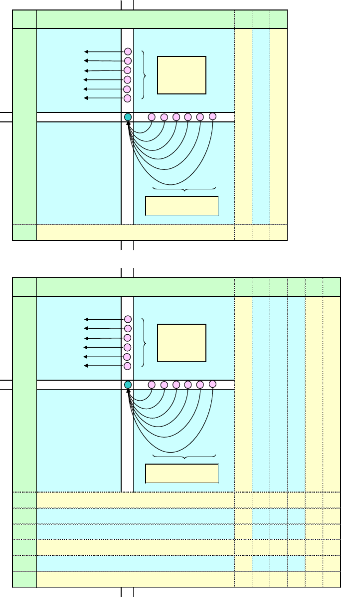
Handbook on Supply and Use Tables and Input-Output Tables with Extensions and Applications
413
Figure A12.1 Transfers made for the product-by-product IOTs
1 2 . . . . . . . . . . . . . . . . . . . . . . . . . . n
1
2
:
:
:
:
:
:
:
:
:
:
:
:
:
:
:
:
:
:
m
1 2 . . . . . . . . . . . . . . . . . . . . . . . . . . n
1
2
:
:
:
:
:
:
:
:
:
:
:
:
:
:
:
:
:
:
m
Industry j
Output of industries at basic prices
Total
SUPPLY TABLE
USE TABLE
Product
i
OUT
IMP
SUP
Industries
Products
Domestic output by product at basic prices
Imports
Total supply at basic prices
Industry
j
Industries
TOT
CON
GCF
Product i
TOT
Intermediate consumption of domestic output at basic prices
Product i produced
elsewhere
Products
Intermediate consumption
Consumption
EXP
FU
SUP
Gross capital formation
Exports
Final uses
Use at basic prices
IMP
Intermediate consumption of imports
TLS
Taxes less subsidies on products
TOT
Intermediate consumption at purchasers' prices
GVA
Gross value added at basic prices
TOT
Output at basic prices
Secondary
product of
industry j
Product i
produced
elsewhere
Secondary
product of
industry
j
Handbook on Supply and Use Tables and Input-Output Tables with Extensions and Applications
414
C. Industry-by-industry IOTs
A12.13 There are two main models for the construction of industry-by-industry IOTs:
• The assumption of a fixed industry sales (FI) structure postulates that each industry has its
own specific sales structure, irrespective of its product mix (model C).
• The alternative assumption of a fixed product sales (FP) structure postulates that each
product has its own specific market shares (deliveries to industries), independent of the
industry where it is produced. The market shares refer to the shares of the total output of a
product delivered to the various intermediate and final users (model D).
A12.14 Rueda-Cantuche and ten Raa (2009), in company with many others, use an encompassing
framework for the construction of industry-by-industry IOTs. The fixed industry sales structure
assumption postulates that all industries have unique input structures, irrespective of the product
market (removal of the second subscript in (2)). Consequently, fixed industry sales coefficients
may be defined accordingly:
=
for all
The supply table needs to be square and negatives may emerge from this assumption.
A12.15 Alternatively, the fixed product sales structure assumption assumes that product 's
unitary deliveries to industry must be independent of the supplier industry . Therefore, all
products require unique industry deliveries, irrespective of the industry of fabrication (removal of
the first subscript in (2)):
=
for all
The supply table does not need to be square and negatives do not emerge from this assumption.
A12.16 It is reasonable to assume that secondary outputs have destinations different from those
of the primary outputs. This is why the fixed product sales structure assumption attracts more
attention in the literature (see Thage and ten Raa (2006) or Yamano and Ahmad (2006)). Moreover,
FP has no negative elements, unlike FI, because of the inversion of the supply table.
A12.17 Canada, Denmark, Finland, the Netherlands, Norway, the United States and OECD are
examples of systems that fully or partially adopt FP to compile industry-by-industry IOTs
(Yamano and Ahmad, 2006).
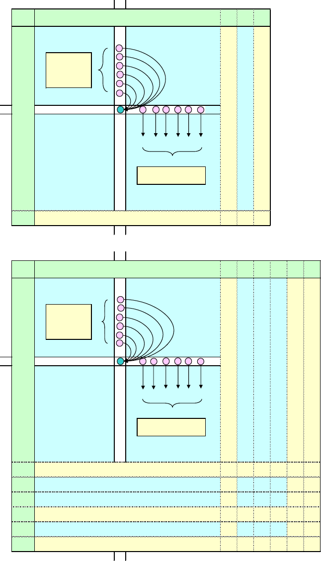
Handbook on Supply and Use Tables and Input-Output Tables with Extensions and Applications
415
Figure A12.2 Transfers made for the industry-by-industry IOTs
1 2 . . . . . . . . . . . . . . . . . . . . . . . . . . n
1
2
:
:
:
:
:
:
:
:
:
:
:
:
:
:
:
:
:
:
m
1 2 . . . . . . . . . . . . . . . . . . . . . . . . . . n
1
2
:
:
:
:
:
:
:
:
:
:
:
:
:
:
:
:
:
:
m
Product
i
SUPPLY TABLE
Industry
j
Industries
OUT
IMP
SUP
Secondary
products of
industry j
Product i
produced
elsewhere
SUP
Products
Intermediate consumption
Consumption
Gross capital formation
Exports
Final uses
Use at basic prices
Industries
TOT
CON
GCF
EXP
Secondary
products of
industry
j
FU
Product i
TOT
Intermediate consumption of domestic output at basic prices
Product
i produced
elsewhere
IMP
Intermediate consumption of imports
TLS
Taxes less subsidies on products
GVA
Gross value added at basic prices
TOT
Intermediate consumption at purchasers' prices
TOT
Output at basic prices
Industry j
USE TABLE
Products
Domestic output by product at basic prices
Imports
Total
Output of industries at basic prices
Total supply at basic prices
Handbook on Supply and Use Tables and Input-Output Tables with Extensions and Applications
416
D. Use of a hybrid technology assumption for product-by-product IOTs
A12.18 The product and the industry technology assumptions represent the two main methods
used for the construction of product-by-product IOTs from SUTs. Although, however, the
assumptions are commonly regarded in the literature as opposites, some national statistical offices
apply hybrid product and industry technology assumptions to produce product-by-product IOTs.
In some cases, the non-negativity of one of the assumptions is enough for it to be used more widely
than a single (non-hybrid) technology assumption. In particular, for hybrid models, the choice of
products for which either the product technology assumption or the industry technology
assumption will be used is mainly based on expert judgements and seldom on empirical analyses.
A12.19 Rueda-Cantuche and ten Raa (2013) present several empirical tests that provide
conclusions on the choice of technology assumption for product-by-product IOTs (such as, in the
construction of the use tables, the assumption that individual establishment data with a full input
specification exist may not be feasible within the tests).
A12.20 Following the expression (1), these authors showed that the tests can provide acceptance
and rejection regions for the competing technology assumptions allowing a hybrid technology
model in which some secondary products are treated by the one assumption and others by the other
assumption. These tests will enable national statistical offices to apply more tailored hybrid
technology assumptions, which can be complemented with expert judgments in order to improve
the entire compilation process.
A12.21 Overall, producers of IOTs should be cautious. The results from these tests should not
lead to rejection of the product technology assumption and the conclusion that it is unrealistic. On
the contrary, the lack of homogeneity in the product classification is constantly biasing final
acceptance or rejection decisions in favour of the competing model (industry technology).
A12.22 It should be noted, however, that detailed product data on inputs and outputs at the level
of individual units are required and valued at basic prices, which are not readily available from
business surveys. Businesses report data on goods and services with insufficient specification and
mostly at purchasers’ prices. There are many examples of partly specified inputs, for example,
single aggregates for a mixed bunch of goods (food and drinks in hotels and restaurants;
consumption of building materials in construction firms; office materials used in businesses, and
others) and the “other costs” items, which may include a large variety of products. It might be
common practice to use assumptions that come close to product or industry technology
assumptions to complete the full specification of firms’ data on inputs and outputs but this should
preferably be carried out with the use of actual data or structures of other firms or establishments
with the same economic activity and similar numbers of workers.
A12.23 Besides, firms report the price paid, including trade and transport margins and (if any)
net taxes on products (purchasers’ prices), so some adjustments need to be applied in order to get
firms’ input data valued at basic prices.
Handbook on Supply and Use Tables and Input-Output Tables with Extensions and Applications
417
A12.24 These tests could lead to statistically significant conclusions on the selection of the most
appropriate technology assumption but the power of the tests might be largely affected by the
heterogeneity in the product classification, the insufficiently detailed breakdown of products and
the measurement errors by the business. These tests may be used as a guide towards the selection
of one of the two technology assumptions in the construction of hybrid technology-based product-
by-product IOTs, for example, as performed by at least one regional statistical office (Catalonia,
Spain).
Handbook on Supply and Use Tables and Input-Output Tables with Extensions and Applications
419
Annex B to chapter 12. Classical causes and treatment of negative cell entries
in the product technology
A. Classical causes of negative elements in the product technology
B12.1 As mentioned in chapter 12, the product technology assumption may generate negative
values because of the systematic negatives in C
-1
and D
-1
. We indicate here the various classical
reasons that were considered for the appearance of negative elements, for example:
• There may be multiple technologies for the production of a product.
• The economic transactions may not fully record technological relations.
• The products may represent heterogeneous elements.
• There may be data errors in the SUTs.
B12.2 In this annex, these factors are briefly reviewed and possible solutions proposed. The
reader is encouraged to consult ten Raa and Rueda-Cantuche (2013) for a thorough review of the
classical issues and available solutions, including algorithmic procedures for the elimination of
negatives which will not be covered in full in this annex.
1. The product technology assumption may be incorrect
B12.3 This means that there is a product that is produced in two different ways. Clearly, there
are cases where this is true, for example in the chemical industry, where there are often different
processes that lead to exactly the same product. Negatives could be created when one process uses
inputs that are not used by another. This assumption is likely to be only valid at a very detailed
level (for example, for kind-of-activity unit or local kind-of-activity unit) and possibly not
applicable at the level of aggregation used in SUTs.
2. Economic transactions are recorded rather than technological relations
B12.4 In principle, the SUTs record all transactions between establishments and enterprises.
These are economic transactions and do not necessarily describe technology. For example, two
companies employ the same process to produce a product. One of the companies subcontracts a
large part of the process, whereas the other company performs the whole process in house. The
two companies will thus show different input structures in the use table for the same output,
possibly leading to negatives.
B12.5 Another situation that could lead to negative elements is where the company operates
vertically integrated production processes. For example, consider the production of cheese at a
dairy farm. The milk produced at the farm and used in the production of cheese is not recorded
Handbook on Supply and Use Tables and Input-Output Tables with Extensions and Applications
420
either as an input or as an output of the dairy farm. Hence, it looks as if the farm produces cheese
without using milk. If the cheese were to be transferred to the dairy industry, and the input structure
of the dairy industry were to be applied to this cheese, a negative input for milk would appear for
the dairy farm.
B12.6 Non-market output creates a special problem in the application of the product technology
assumption. Non-market output is valued by convention as the sum of the costs incurred in its
production, with net operating surplus being zero. This is applied at the level of the producing unit
and not by product. Secondary market products are valued at their market prices but the value of
the total output of the unit is determined by the costs. If, therefore, the secondary products are
transferred to the (market) industry where it is produced as primary product, a negative may arise
for the net operating surplus.
3. Heterogeneity in data and classifications
B12.7 Negatives can be generated by heterogeneity in the data. Heterogeneity is unavoidable
because products and industries need to be aggregated in SUTs. In the numerical example used in
this chapter, the manufacturing products produced by agriculture could be totally different
products from – or perhaps a subset of – the products produced by the manufacturing industry. It
is clear that assuming the product technology in such a case would create problems. It is
recommended therefore that the product technology assumption should always be applied at the
most detailed level of products possible, allowing for the requirement of square SUTs.
B12.8 The classifications play an important role here. As mentioned earlier, the international
classifications may be based on a variety of criteria that are not always the most appropriate for
input-output analysis. An example is footwear. The CPC does not distinguish footwear of different
materials. More important, it provides a distinction of footwear by use. Aggregating leather and
plastic shoes in a single column of the SUTs would, however, create heterogeneity in the
description of the production processes and may lead to negatives when another industry produces
one of the two types of shoes as secondary output.
4. Errors in the SUTs data
B12.9 Last but not least, negatives can be caused by errors in the SUTs starting point for
transformation or parts of the transformation itself, in terms of the trade margins, transport
margins, taxes on products and subsidies on products.
B12.10 This is an important consideration, because it could provide insights about the quality of
the elements of the SUTs system. In this way, the compilation of the IOTs can provide a useful
and powerful feedback loop for checking the plausibility of the SUTs data. This experience has
shown that IOTs should be compiled simultaneously with SUTs to enable the results of the IOTs
to be immediately incorporated back into the SUTs. This approach may not hold when a long run
Handbook on Supply and Use Tables and Input-Output Tables with Extensions and Applications
421
of SUTs need to be revised as a consequence of methodological changes or a new ISIC or a new
SNA.
B. Overall strategy for removing negatives
B12.11 As already indicated, the negatives in model A and model C have a structural cause. If it
use of these models is mandatory, there are various empirical ways to resolve these negatives.
B12.12 Ideally, all the negatives should be removed manually, once the cause of the negatives
has been identified, and the SUTs and IOTs rebalanced, as appropriate. If, however, the available
resources, time or information are limited, alternative strategies for resolving these negatives may
need to be applied. For example, model A is applied and negative cell entries are generated and a
three-step approach could be applied:
• All large, or significant, negative cell entries are investigated, resolved and rebalanced –
these changes could affect the SUTs or any of the steps in the transformation to the IOTs. In
this process, some positive cell entries may be identified as implausible and may also need
to be changed.
• Small negatives are eliminated by applying some form of automated procedure.
• The plausibility of the results is reviewed and changes are made, if necessary.
C. Specific approaches to dealing with negatives
B12.13 There are various ways of dealing with negatives, including:
• Merging industries
• Changing the primary producer
• Applying industry technology within the product technology framework
• Introducing new products
• Correcting errors in the SUTs
• Making manual corrections to IOTs
• After the above steps, using the Almon method used to remove any small negative cell
entries
1. Merging industries
B12.14 If two or more products are produced more or less simultaneously, it is often difficult to
distinguish the processes by which they were produced. For example, two closely related industries
Handbook on Supply and Use Tables and Input-Output Tables with Extensions and Applications
422
are restaurants (ISIC Rev. 4, group 561) and bars (ISIC Rev. 4, group 563). Restaurants will have
substantial secondary output of beverage serving services (CPC Version 2.1, group 634, the main
product of bars), while bars will have considerable secondary output of food serving services (CPC
Version 2.1, group 633, the main product of restaurants). It will be difficult to distinguish separate
input structures for beverage serving services and food serving services, since both services are
usually provided simultaneously, essentially constituting a form of joint production. Trying to
distinguish separate input structures by applying the product technology may lead to negative
elements.
B12.15 It would be better to aggregate such industries and hence the products before applying
the product technology. The assumption is then that both products are produced in the same
production process – this is far from ideal and not in line with the recommended approach, to
operate at the most detailed level possible. Merging the industries removes the secondary outputs
and prevents negatives, and can offer a convenient solution to many cases. The apparent
disadvantage of increasing the heterogeneity of the database is in fact not so important, since the
input structures that are being merged are in any event similar.
2. Changing the primary producer
B12.16 It was noted that it is essential to know which industry is the primary producer for each
product if the product technology assumption is applied. In some cases, negatives are created
because the initially chosen primary producer of a product is not the right one (for example,
research and development). In such a case, the input structure of another industry might be more
appropriate for use as the starting point.
B12.17 It must be noted that, in most cases, there are many more products than industries, and
hence there can be products in respect of which it is not immediately obvious who the primary
producer may be, in particular when the products are fairly heterogeneous.
3. Apply industry technology within the product technology framework
B12.18 In the event that the product technology is not valid because there are in fact two ways
of producing a product, the resulting problem may be resolved by applying the industry technology
assumption. The industry technology assumption posits that all products produced by the industry
are produced in the same production process. Thus it does not matter, for example, whether the
outputs of the agriculture industry are called agricultural products or manufacturing products, they
can all be treated as if they were primary products. The secondary output of manufacturing
products could thus be added to the primary output. However, the same adjustments have to be
made in the use table: in other words, the corresponding amounts have to be transferred from the
manufacturing products row to the agricultural products row and these amounts have to be
allocated to the appropriate users. It is easy to see that this problem is precisely the same as that
encountered when compiling industry-by-industry IOTs. If available, actual data could be used in
support of this assumption.
Handbook on Supply and Use Tables and Input-Output Tables with Extensions and Applications
423
B12.19 The drawback of this solution is that it leads to a reclassification of products. The heading
“agricultural products” in the IOTs would no longer encompass the same products as the same
heading in SUTs. This could pose problems for interpretation and for users. In that case, this
solution could still be applied in cases where the reclassification stays within the product groups
distinguished in the most detailed published tables.
4. Introducing new products
B12.20 Another possibility is to introduce a new product. It could well be that there are two or
more ways to produce a given product. If there is sufficient information on the different production
processes available, this could be added to strengthen the homogeneity of the IOTs. The drawback
of this method is that it is relatively labour and data-intensive. If, however, all products are defined
as characteristic in the industry where they are actually produced, then the product technology is
in practice replaced by an industry technology.
5. Correcting errors in the SUTs
B12.21 Wherever it can be established that negatives (or other implausible results) are caused by
errors, these should of course be repaired by correcting the data.
B12.22 The problem here is that IOTs are usually compiled after the closing of the accounts and
the SUTs. This is more often the case in countries where IOTs are compiled less regularly, for
example, once every five years. In such cases, when the compilation of the IOTs reveals problems
or errors in the SUTs, these can often only be resolved at the next benchmark revision and therefore
inconsistencies may have to be reflected to produce plausible IOTs.
6. Making manual corrections to IOTs
B12.23 Lastly, if large negatives remain that cannot be dealt with by any of the above solutions,
for example, because it would significantly affect the compatibility with the original SUTs, they
could be resolved by manually correcting the results of the product technology.
B12.24 After the large negative values have been removed and, where applicable, after manually
adjusting some clearly incorrect positive elements, the remaining small negatives can also be
eliminated by setting them to zero, as in Armstrong (1975). The final balancing to match the totals
can be carried out with the use of a mathematical routine such as the RAS procedure or other
methods as covered in chapter 18 of this Handbook. This is the case when these negatives may be
considered to be the normal “noise” in the compilation process, due to unavoidable heterogeneity
and statistical error within the normal confidence ranges.
7. Almon method
B12.25 Depending upon the diversity of industries’ secondary activities, model A (product
technology assumption) may generate product-by-product IOTs with negative entries.

Handbook on Supply and Use Tables and Input-Output Tables with Extensions and Applications
424
B12.26 Almon developed an alternative method which is consistent with the product technology
assumption but calculates product-by-product IOTs from SUTs without any negative entries
(Almon, 2000). The most effective application of the Almond method should be considered when
all of the above procedures have been used, and the focus is only to remove the last small suite of
negative entries. The Almond method should not be used alone and directly applied to the original
SUTs.
B12.27 The method applies the product technology by calculating IOTs row by row and taking
care of negatives as soon as they appear. It monitors the transformation process outlined for model
A in a step-by-step manner for each row (in other words, product) and, when a negative cell entry
occurs, the amounts transferred are reduced until the negative value is absorbed.
B12.28 The method leaves the row totals unaffected but there is no guarantee that the column
totals are maintained. It is therefore necessary to perform a RAS procedure or a similar procedure
to rebalance the row and column totals.
B12.29 The fact that no negative cell entries appear also means that the negative cell entries
cannot be used to analyse the quality and plausibility of the SUTs. The results of the Almon method
can, however, be checked by recalculating the use table. In a manner similar to that outlined above,
this check provides information, such as on areas where the structure of SUTs or the product
assumptions can be improved.
B12.30 Box B12.1 shows the application of the Almon method in removing small negatives for
a small numerical example.
Box B.1 Almon method
Clopper Almon developed a method (Almon, 2000) to compile product-by-product IOTs from SUTs using the
product technology assumption without negative cell entries.
In scenario A, the traditional transformation of the SUTs to IOTs with the product technology assumption
(model A) does not result in negative flows. A marginal change in the use table in scenario B does, however,
result in negative cell entries.
In scenario A, the Almon method generates the same result as the traditional transformation with model A. In
Scenario B, however, it is demonstrated how negative cell entries can be avoided by using the Almon
procedure.
The final result of the Almon method reflects the fact that rennet is only used in the cheese industry. In addition,
the Almon procedure gives an indication in the sheet “New use table” of the manner in which the use table can
be revised to avoid negative cell entries in the compiled product-by-product IOTs. In fact, in the example
adduced by Almon, the “New use table” of scenario B corresponds with the original use table of Scenario A.

Handbook on Supply and Use Tables and Input-Output Tables with Extensions and Applications
425
Supply table Supply table
Cheese Ice Cream Chocolate Rennet Other Cheese Ice Cream Chocolate Rennet Other
Cheese
70 30 100 Cheese 70 30 100
Ice Cream 20 180 200 Ice Cream 20 180 200
Chocolate 100 100 Chocolate 100 100
Rennet 20 20 Rennet 20 20
Other 535 535 Other 535 535
90 210 100 20 535 90 210 100 20 535
Use table Use table
Cheese
Ice Cream
Chocolate Rennet Other Cheese Ice Cream Chocolate Rennet Other
Cheese 100 100 Cheese 100 100
Ice Cream 200 200 Ice Cream 200 200
Chocolate 4 36 60 100 Chocolate 3 37 60 100
Rennet 14 6 20 Rennet 15 5 20
Other 28 72 30 5 400 535 Other 28 72 30 5 400 535
44 96 70 15 535 760 44 96 70 15 535 760
90 210 100 20 535 760 90 210 100 20 535 760
Product-by-product input-output table Product-by-product input-output table
Cheese
Ice Cream
Chocolate Rennet Other Cheese Ice Cream Chocolate Rennet Other
Cheese
100 100 Cheese 100 100
Ice Cream 200 200 Ice Cream 200 200
Chocolate 40 60 100 Chocolate -1.67 41.67 60 100
Rennet 20 20 Rennet 21.67 -1.67 20
Other 30 70 30 5 400 535 Other 30 70 30 5 400 535
50 90 70 15 535 760 50 90 70 15 535 760
100 200 100 20 535 760 100 200 100 20 535 760
Product-by-product input-output table Product-by-product input-output table
Cheese
Ice Cream Chocolate Rennet Other Cheese Ice Cream Chocolate Rennet Other
Cheese 100 100 Cheese 100 100
Ice Cream 200 200 Ice Cream 200 200
Chocolate 40 60 100 Chocolate 40 60 100
Rennet 20 20 Rennet 20 20
Other 30 70 30 5 400 535 Other 30 70 30 5 400 535
50 90 70 15 535 760 50 90 70 15 535 760
100 200 100 20 535 760 100 200 100 20 535 760
New use table
New use table
Cheese Ice Cream
Chocolate Rennet Other Cheese Ice Cream Chocolate Rennet Other
Cheese 100 100 Cheese 100 100
Ice Cream 200 200 Ice Cream 200 200
Chocolate 4 36 60 100 Chocolate 4 36 60 100
Rennet 14 6 20 Rennet 14 6 20
Other 28 72 30 5 400 535 Other 28 72 30 5 400 535
44 96 70 15 535 760 44 96 70 15 535 760
90 210 100 20 535 760 90 210 100 20 535 760
SCENARIO A
SCENARIO B
Industries
q
Industries
q
Industries
y
q
Products
Products
Products
Products
Industries
y
q
g'
g'
Y
q
Products
Y
q'
Products
Almon procedures
Almon procedures
Products
Y
q
Products
q'
Y
q
Products
Products
Y
q
Products
Products
Products
Y
q
Products
Products
W
g'
W
g'
W
W
Product technology assumption
Product technology assumption
q
Products
g'
W
g'
W
q'
W
q'
W

Handbook on Supply and Use Tables and Input-Output Tables with Extensions and Applications
427
Annex C to chapter 12. Examples of reviews of approaches to the treatment of
secondary products
Treatment of secondary products
Year Source or author(s) as appropriate Reference to specific pages
Transfer of outputs only
Transfer method
1961
Stone
Pages 39–41
1973
United Nations
Page 25
1985
Fukui and Seneta
Page 178
1986
Viet
Pages 16–18
1990
Kop Jansen and ten Raa
Page 215
1994
Viet
Pages 36–38
Stone method or by-product technology model
1961
Stone
Pages 39–41
1973
United Nations
Page 26
1984
Ten Raa, Chakraborty and Small
Page 88
1985
Fukui and Seneta
Page 178
1986
Viet
Pages 15–16
1990
Kop Jansen and ten Raa
Page 215
1994
Viet
Page 38
European System of Integrated Economic Accounts (ESA) Method (EUROSTAT, 1979)
1986
Viet
Pages 18–19
1990
Kop Jansen and ten Raa
Page 214
1994
Viet
Pages 38–40
TRANSFER OF INPUTS AND OUTPUTS
Lump-sum or aggregation method
1974
Office for Statistical Standards
Page 116
1985
Fukui and Seneta
Page 177
1990
Kop Jansen and ten Raa
Page 214
1994
Viet
Pages 42–43
Methods with a single technology assumption – product technology model
1968
United Nations
Pages 48–51
1968
van Rijckeghem
Pages 607–608
1970
Gigantes
Pages 280–284
1973
United Nations
Pages 26–32
1975
Armstrong
Pages 71–72
1984
Ten Raa, Chakraborty and Small
Page 88

Handbook on Supply and Use Tables and Input-Output Tables with Extensions and Applications
428
1986
Viet
Page 20
1990
Kop Jansen and ten Raa
Page 215
1994
Viet
Page 41
Methods with a single technology assumption – industry technology model
1968
United Nations
Pages 48–51
1970
Gigantes
Pages 272–280
1973
United Nations
Pages 26–32
1975
Armstrong
Pages 71–72
1984
Ten Raa, Chakraborty and Small
Pages 88–89
1985
Fukui and Seneta
Page 178
1986
Viet
Page 21
1990
Kop Jansen and ten Raa
Page 215
1994
Viet
Pages 40–41
Methods with a single technology assumption – activity technology model
1994
Konijn
Pages 143–184
1995
Konijn and Steenge
Pages 426–433
Hybrid technology assumption methods – mixed product and industry technology assumptions
1968
United Nations
Pages 48–51
1970
Gigantes
Pages 284–290
1973
United Nations
Pages 33–34
1975
Armstrong
Pages 72–76
Hybrid technology assumption methods – product technology assumption and by-product technology
method
1984
Ten Raa, Chakraborty and Small
Page 90
Handbook on Supply and Use Tables and Input-Output Tables with Extensions and Applications
429
Chapter 13. Compiling physical supply and use tables and environmentally
extended input-output tables
A. Introduction
13.1 Industrial growth and a rapidly growing world population are having a major impact on the
global environment and allocation of material resources. Most changes in the environment are
brought about by human activities and these activities result in a flow of materials. The flow of
resources from the natural environment to the economy is a prerequisite of production, while flows
of residuals from the economy to the environment are the consequence of production and
consumption. A full understanding of these processes requires a complete description of the
physical dimension of the economy and its interaction with the environment.
13.2 PSUTs and EE-IOTs are used to describe the magnitude (measured by tons or other
physical measuring units) and the nature of materials and products flowing in the economy, within
the economy and between the economy and nature. They show how the natural resources (natural
inputs) enter, are processed and subsequently, as products, are moved around the economy, used
and finally returned to the natural environment in the form of residuals (emissions, waste, waste
water, and so forth). The exchange of products between the domestic economy and the rest of the
world is also described in the PSUTs and EE-IOTs.
13.3 The SEEA Central Framework (United Nations, FAO, IMF, OECD and World Bank, 2014)
sets out the internationally agreed standard concepts, definitions, classifications, accounting rules
and tables for producing internationally comparable statistics for environmental-economic
accounts. The SEEA is fully consistent with the SNA. It uses an accounting structure and concepts,
definitions and classifications consistent with the SNA in order to facilitate the integration of
environmental and economic statistics.
13.4 The SEEA Central Framework describes a set of accounts that are relevant for the analyses
of the interactions between the environment and the economy. The present chapter focuses on the
compilation of PSUTs and the EE-IOTs. Section B presents the structure of PSUTs and the relevant
definitions and classifications of natural inputs and residuals. This section also covers the
accounting and balancing identities and the principles of physical flow accounting. Section C
covers the compilation steps for PSUTs and the way in which they fit into the overall process
provided in chapter 3 of this Handbook. This section will also cover the data sources potentially
used for the compilation of PSUTs.

Handbook on Supply and Use Tables and Input-Output Tables with Extensions and Applications
430
13.5 Section D describes how to extend standard economic IOTs in monetary units to include
information on the environment in physical units in the environmental extended IOTs. This section
focuses on two types of EE-IOTs, namely the single region IOTs and the hybrid IOTs. The
compilation steps for EE-IOTs are described in section E. Two country examples on the
compilation of PSUTs are presented at the end of section F.
13.6 The presentation of the material in this chapter does not necessarily reflect the order of
compilation of PSUTs and environmental extended IOTs recommended to countries. The
compilation of environmental accounts in general, and more specifically of the PSUTs and EE-
IOTs, is carried out in a gradual manner, starting with the compilation of those modules of the
2012 SEEA that reflect countries’ priorities and resource availability. Given the scope of the 2012
SEEA, it is not possible to provide detailed practical guidance for compilation of the accounts for
the various environmental domains (such as water, energy, forestry and others) in this Handbook.
The aim of this chapter, therefore, is rather to provide the conceptual link of the PSUTs and EE-
IOTs with the compilation of the SUTs and IOTs of the SNA, showing how to mainstream their
compilation with that of SUTs and IOTs. More guidance on the compilation of the accounts may
be found on the website of the United Nations at https://seea.un.org, and Eurostat at
http://ec.europa.eu/eurostat/web/environment/methodology. Box 13.1 also presents a list of
selected reference material.
13.7 Physical IOTs are also an extension of the SUTs framework designed to take into account
environmental considerations. They consist of a transformation of the PSUTs into physical IOTs,
although, because of the difficulties, conceptual and practical, in the compilation of physical IOTs,
the focus of the 2012 SEEA has shifted more towards the compilation of EE-IOTs rather than
physical IOTs. One conceptual disadvantage of the physical IOTs, for example, is that they do not
allow for a distinction between different types of inputs and outputs. Inputs of products and natural
inputs are combined together in physical IOTs to generate a single output, which combines
products and residuals. This limits the environmental analyses that can be made by combining
physical accounts. On the practical side, the choice of the physical unit used to measure the various
types of products, natural inputs and residuals is also not simple. This chapter, therefore, does not
elaborate further on the compilation of physical IOTs, although some countries do in fact compile
them; from this point on in the Handbook, the focus will be primarily on EE-IOTs as opposed to
physical IOTs.
B. Overview of PSUTs
13.8 The SEEA provides the conceptual foundation for the extensions of the SNA that will
include the environment. The SEEA Central Framework records flow from the environment to the
economy (natural input), within the economy (product flows), and from the economy to the
environment (residuals). Figure 13.1 provides a schematic representation of the physical flows of
natural inputs, products and residuals between the environment and the economy.

Handbook on Supply and Use Tables and Input-Output Tables with Extensions and Applications
431
Figure 13.1 Physical flows of natural inputs, products and residuals
Source: SEEA 2012 Central Framework.
13.9 PSUTs record physical flows of natural inputs, products and residuals in physical units of
measurement. They are used to assess how an economy supplies and uses natural resources and
they examine changes in production and consumption patterns over the accounting period. In
combination with data from monetary SUTs, they allow for analyses of changes in productivity
and intensity in the use of natural inputs and the release of residuals. Physical flows within the
environment, namely, natural flows of materials and energy, lie outside the scope of PSUTs.
13.10 For the recording of physical flows, the structure of the SUTs of the SNA is extended by
additional rows and columns in order to accommodate physical flows between the economy and
the environment.
13.11 As shown in Table 13.1, PSUTs consist of a pair of tables which have the same format or
structure. By row, the two tables show the various physical flow types, namely natural inputs,
products and residuals. By column, they show the various origins and destinations supplying and
using the flow items, namely industries (production activities), households (consumption
activities), accumulation (changes in stocks of produced assets and product inventories), the rest
of the world and the environment.
13.12 The physical supply table shows which physical flows are provided by which source
(industries, households, accumulation, rest of the world, or the environment). In other words, it
shows the physical flows by origin. The physical use table shows where the physical flows are
used or received (namely, production, consumption, accumulation activity and others). In other
words, it shows the physical flows by destination. The SEEA Central Framework notes that the
general framework shown in Table 13.1 may be articulated either fully or partly.

Handbook on Supply and Use Tables and Input-Output Tables with Extensions and Applications
432
Table 13.1 General PSUT
9
13.13 As indicated in chapter 2, the section of the PSUTs related to products provides the physical
measurements of the flows that are recorded in the monetary SUTs presented in previous chapters.
Many of the flows of products recorded in monetary terms relate to the use of products originating
from the environment, for example, the manufacture of wood products, or to activities and
expenditures associated with the environment, for example, environmental protection expenditure.
It should be noted that the monetary and physical SUTs of the SEEA are compiled for either a
specific underlying environmental theme or for an entire range of environmental themes. This
means that the industry and product breakdown shown in the tables explicitly identify the relevant
industries and products for the environmental theme in question. For example, when compiling
SUTs for water in physical and monetary units, the industry breakdown will explicitly identify the
industry distributing water, the industry treating wastewater and the major industries abstracting
and using water. Similarly, on the product side, the relevant products for water will be explicitly
9
Based on table 3.2.1 of the SEEA 2012 Central Framework
Agriculture,
forestry, etc.
Mining and
quarrying
…
Services
Mineral and energy resource
Water
…
Agriculture, forestry, etc.
Ores and minerals; etc.
…
Services
Solid waste
Wastewater
…
Simplified structure of the physical supply table
Total supply
by residuals
(TSR)
Total Supply
Residuals
Residuals generated by industry
(I)
Residuals
received
from the rest
of the world
(L)
Residuals
generated
by final
consumtpion
(J)
Residuals from
scrapping and
demolition of
produced assets
and emissions
from controlloed
landfill sites
( K)
Residuals
recovered
from the
environment
(M)
Products
Output by product by industry
(C)
Imports by
product
(D)
Total supply
by product
(TSP)
Total
Natural
inputs
Flows from
the
environment
(A)
Total supply
by natural
inputs
(TSNI)
Industries
Industries
Imports
Final
consumption
Gross capital
formation/accu
mulation
Environment
Agriculture,
forestry, etc.
Mining and
quarrying
… Services
Mineral and energy resource
Water
…
Agriculture, forestry, etc.
Ores and minerals; etc.
…
Services
Solid waste
Wastewater
…
Total Use
Empty by definition Blank cells may contain relevant flows
Simplified structure of the physical use table
Residual
flows direct
to the
enviornment
(Q)
Total use by
residuals
(TUR)
Total use by
product
(TUP)
Residuals
C ollection and treatment of waste and other
residuals
(N)
Residuals
sent to the
rest of the
world
(P)
Accumulation of
waste in
controlled
landfilled
(O)
Natural
inputs
Extraction of natural inputs
(B)
Total use by
natural
inputs
(TUNI)
Products
Intermediate consumption by product and by
industry
(E)
Exports by
product
(H)
Final
consumption
by product
and by
category
(F)
Gross capital
formation/accu
mulation
(G)
Industries
Industries
Exports
Final
consumption
Gross capital
formation/accu
mulation
Environment
Total
Handbook on Supply and Use Tables and Input-Output Tables with Extensions and Applications
433
identified. The monetary and physical tables are therefore compiled with the same breakdown, and
indicators can be calculated using consistent physical and monetary information.
(a) Natural inputs, products and residuals
13.14 The starting point for understanding the PSUTs is to have a clear understanding of the
terminology used in the construction of such tables. The definition of products is the same as that
used within the national accounts, namely that products (goods and services) are the result of
production. They are exchanged and used for various purposes: as inputs in the production of other
goods and services, as final consumption or for investment (2008 SNA, para. 2.36). Natural inputs
and residuals do not fall within the national accounts boundaries but are defined in the SEEA
Central Framework in order to account for the physical interrelations between the national
economy and the natural environment.
13.15 Natural inputs are all physical inputs that are moved from their location in the environment
as a part of the economic process, or are directly used in production. They include natural timber
resources and water resources that are extracted from the environment. Natural inputs should not
be confused with products. In the case of mining activities, for example, natural inputs, such as
gross ore, are input flows to the mining industry and only become products once they are an output
of the mining industry, such as processed ore and concentrates.
13.16 The three broad classes of natural inputs are distinguished in the SEEA and listed below.
Table 13.2 provides the classes of natural input as defined by the SEEA Central Framework:
(a) Natural resource inputs: these are material resources extracted from the natural
environment. They include materials actually used in production, and also natural resource
residuals, which are natural resource inputs that do not subsequently become products but
instead return immediately to the environment;
(b) Natural inputs of energy from renewable sources: these include inputs such as solar and
hydro energy captured by economic units;
(c) Other natural inputs: these include inputs such as those from soil (for example, soil
nutrients) and from air (for example, oxygen taken up in combustion processes and carbon
dioxide absorbed by cultivated plants).

Handbook on Supply and Use Tables and Input-Output Tables with Extensions and Applications
434
Table 13.2 Classes of natural input
13.17 Residuals refer to flows of solid, liquid and gaseous materials and energy that are
discarded, discharged or emitted by the economy and households to the environment (for example,
emissions to air and water) through processes of production, consumption and accumulation. The
SEEA Central Framework distinguishes the following groups of residuals:
(a) Solid waste: this covers discarded materials that are no longer required by the owner or
user. Solid waste includes materials that are in a solid or liquid state but excludes
wastewater and small particulate matter released into the atmosphere;
(b) Wastewater: this is discarded water that is no longer required by the owner or user. Water
discharged into drains or sewers, water received by water treatment plants and water
1
1.1
1.1.1
1.1.1.1 Oil resources
1.1.1.2 Natural gas resources
1.1.1.3
Coal and peat resources
1.1.1.4 Non-metallic mineral resources (excl. coal & peat resources)
1.1.1.5 Metallic mineral resources
1.1.2
1.1.3
1.1.4
1.1.5
1.1.6
1.1.6.1
Surface water
1.1.6.2 Groundwater
1.1.6.3 Soil water
1.2
2
2.1
2.2
2.3
2.4
2.5
2.6
3
3.1
3.1.1
3.1.2
3.1.3
3.2
3.2.1
3.2.2
3.2.3
3.2.4
3.3
Natural resource inputs
Extraction used in production
Mineral and energy resources
Soil resources (excavated)
Natural timber resources
Natural aquatic resources
Other natural biological resources (excluding timber and aquatic resources)
Water resources
Natural resource residuals
Inputs of energy from renewable sources
Solar
Hydro
Wind
Wave and tidal
Geothermal
Other electricity and heat
Other natural inputs
Inputs from soil
Soil nutrients
Soil carbon
Carbon dioxide
Other inputs from air
Other natural inputs n.e.c.
Other inputs from soil
Inputs from air
Nitrogen
Oxygen
Handbook on Supply and Use Tables and Input-Output Tables with Extensions and Applications
435
discharged directly into the environment is all considered wastewater. Wastewater includes
return flows of water which are flows of water directly into the environment, with or
without treatment. All water is included, regardless of its quality, including returns from
hydroelectric power generators;
(c) Emissions: these are substances released into the environment by establishments and
households as a result of production, consumption and accumulation processes. Generally,
emissions are analysed by type of receiving environment (air, water and soil) and by type
of substance, as further defined below:
(i) Emissions to air: these consist of gaseous and particulate substances released into
the atmosphere by establishments and households as a result of production,
consumption and accumulation processes;
(ii) Emissions to water: these are substances released into water resources by
establishments and households as a result of production, consumption and
accumulation processes;
(iii) Emissions to soil: these are substances released into the soil by establishments and
households as a result of production, consumption and accumulation processes;
(d) Dissipative uses of products: this covers products that are deliberately released into the
environment as part of production processes. For example, fertilizers and pesticides are
deliberately spread on soil and plants as part of agricultural and forestry practice, and in
some countries salt is spread on roads to improve road conditions for drivers;
(e) Dissipative losses: these are material residues that are an indirect result of production and
consumption activity. Examples include particulate abrasion from road surfaces, abrasion
residues from car brakes and tyres, and zinc from rain collection systems;
(f) Natural resource residuals: these are natural resource inputs that do not subsequently
become incorporated into production processes and instead return immediately to the
environment. Natural resource residuals are recorded as a generation of residuals by natural
resource extracting industries and as a flow of residuals directly into the environment.
These flows therefore do not become products nor do they enter the economy. An example
of a natural resource residual is cooling water which is abstracted to cool plants such as
electricity generation plants, chemical manufacturing plants, and others. Once the water
cools the plant, it is returned generally into the same place in the environment. It is
important to monitor these residuals because of their environmental impact.
13.18 Table 13.3 provides examples of the types of materials and components that are commonly
included in the different groups of residuals for analytical purposes, depending on whether the
focus of the analysis is on the purpose behind the discard (for example, solid waste), the destination

Handbook on Supply and Use Tables and Input-Output Tables with Extensions and Applications
436
of the substance (for example, emissions to air), or the processes leading to the emission (for
example, dissipative losses).
Table 13.3 Typical components for groups of residuals
10
* This list of typical components for groups of residuals can also be applied to certain flows defined as products.
13.19 Another way in which residuals are considered is in terms of losses. This is of particular
interest in the analysis of physical flows of energy and water. Four types of losses are identified
according to the stage at which they occur within the production process:
(a) Losses during extraction are those that occur during extraction of a natural resource before
there is any further processing, treatment or transportation of the extracted natural resource.
Losses during extraction exclude natural resources that are re-injected into the deposit from
which they were extracted;
(b) Losses during distribution are losses that occur between a point of abstraction, extraction
or supply and a point of use;
(c) Losses during storage are losses of energy products and materials held in inventories. They
include evaporation, leakages of fuels (measured in mass or volume units), wastage and
accidental damage. Excluded from the scope of inventories are non-produced assets, even
though they might be considered as being stored;
(d) Losses during transformation refer to the energy lost, for example in the form of heat,
during the transformation of one energy product into another.
10
Table 3.2.4 of the SEEA 2012 Central Framework
Handbook on Supply and Use Tables and Input-Output Tables with Extensions and Applications
437
(b) Accounting and balancing identities
13.20 As explained in chapters 1 and 2, SUTs are linked together through various accounting and
balancing identities. PSUTs, which represent the environmental extensions of the SNA-based
SUTs in physical terms, also include a range of important accounting and balancing identities. The
starting point for the balancing of the PSUTs is the supply and use of product identity, which
recognizes that, within the economy, the amount of a product supplied must be equal in physical
units to that used within the economy or exported. Thus:
Total supply of products (TSP) = Total use of products (TUP)
where
Total supply of products (TSP) = Domestic production (C) + imports (D)
Total use of products (TUP) = Intermediate consumption (E) + household final
consumption (F) + gross capital formation (G) + exports (H)
The references in parentheses relate to specific parts of the PSUTs illustrated in Figure 13.1.
13.21 In the PSUTs, the supply and use of product identity also holds in physical units for flows
of natural inputs and residuals:
Total supply of natural inputs (TSNI) = Total use of natural inputs (TUNI)
Total supply of residuals (TSR) = Total use of residuals (TUR)
13.22 These identities also relate to the fundamental physical law underpinning the PSUTs,
namely the conservation of mass and energy. These physical identities imply the existence of
material and energy balances for all individual materials within the system. It can be demonstrated
that, over an accounting period, the following is true:
Flows of materials into an economy must equal the flows of materials out of an economy, plus
any net additions to stock in the economy.
This is known as the input-output identity.
13.23 The net additions to the stock comprise additions and deductions over an accounting period
in:
(a) Gross capital formation in investment goods and inventories of products;
(b) Physical flows of residuals to and from the rest of the world;
(c) Residuals recovered from the environment (for example, oil collected following an oil
spill);
Handbook on Supply and Use Tables and Input-Output Tables with Extensions and Applications
438
(d) Accumulation of solid waste in controlled landfill sites (excluding emissions from these
sites).
13.24 Thus, the input-output identity describing the physical flows between an economy and the
environment may represented as follows:
Materials into the economy = Materials out of the economy + Net additions to stock in the
economy
where
Materials into the economy = Natural inputs (A) + Imports (D) + Residuals received from
the rest of the world (L) + Residuals recovered from the environment (M)
Materials out of the economy = Residual flows to the environment (Q) + Exports (H) +
Residuals sent to the rest of the world (P)
Net additions to stock in the economy = Gross capital formation (G) + Accumulation in
controlled landfill sites (O) - Residuals from produced assets and controlled landfill sites
(K)
13.25 This identity can be applied at the level of an entire economy and also at the level of an
individual industry or household, in which case the notion of imports and exports refers to flows
to and from other industries in the economy and also those to and from the rest of the world.
13.26 Natural resource residuals are recorded in the PSUTs, first as a supply from the
environment and use of natural inputs by the economy (parts (A) and (B) in Table 13.1) and then
as returning flow to the environment (parts (I) and (Q) in Table 13.1). Accordingly, unlike natural
inputs, they do not become products and are not recorded in the block of rows for products in the
PSUTs.
13.27 PSUTs can be compiled for a single specific environmental domain such as water or
energy, but also for a larger set of domains. In either case, these accounting identities and a
common set of accounting principles can be applied. In particular, clear boundaries must be
established in respect of the point of transition between the environment and the economy.
(c) Recording principles of physical flow accounting
13.28 When compiling PSUTs there are specific recording principles that should be followed, in
particular with regard to the gross and net recording of physical flows, the treatment of
international flows of goods, and the treatment of goods for processing. These are described below.
Handbook on Supply and Use Tables and Input-Output Tables with Extensions and Applications
439
(i) Gross and net recording of physical flows
13.29 PSUTs record flows between the environment and the economy, flows between different
economic units and, where applicable, flows within economic units. This recording of flows is
referred to in the SEEA as “gross recording”. The main advantage of a gross recording approach
is that a full reconciliation of all flows at all levels of the SUTs, for example, by industry and by
product, can be made.
13.30 Recording all of these flows may, however, hide some key relationships so, for analytical
purposes, alternative consolidations and aggregations of flows have been developed. These
alternative approaches are often referred to as “net recordings”, although the nature of the
consolidations and aggregations varies and there is therefore no single application of net recording.
13.31 One example of the difference between gross and net recording is that of PSUTs for energy.
When PSUTs for energy are compiled on a gross basis, they show all flows of energy between
economic units. Some of these are flows of energy products to energy producers which transform
one energy product into a different one (the burning of coal to generate electricity in electric power
plants is one example) while other flows are destined for end-users (as is the case with delivery of
electricity to households). PSUTs on the basis of net recording exclude non-consumptive energy
use, which is the transformation of one energy product into another product, thus allowing for a
greater focus on the end use of energy.
13.32 Generally, care should be taken when using and interpreting the terms “gross” and “net”
and clear definitions of inclusions and exclusions should be sought and provided.
(ii) Treatment of international flows
13.33 The treatment of physical flows to and from the rest of the world needs careful articulation.
In line with the SNA, the underlying principle applied in the SEEA is that relevant flows are
attributed to the country of residence of the producing or consuming unit. This differs from the
territory-based principle of recording, which is applied in a number of statistical domains such as
energy statistics and energy balances. This principle attributes the relevant flows to the country in
which the producing or consuming unit is located at the time of the flow.
13.34 In accordance with both the 2008 SNA and BPM 6, the residence of an institutional unit is
determined by the economic territory with which it has the strongest connection (2008 SNA, paras.
4.10–4.15). In the majority of situations, the concepts of territory and residence are closely aligned.
Nevertheless there are cases that require careful consideration in order to choose the appropriate
recording. These include international transport, tourist activity and natural resource inputs, as
further explored below.
13.35 International transport: to ensure consistency with other sections of the accounts, the
appropriate recording of international transport activity is centred on the residence of the operator
Handbook on Supply and Use Tables and Input-Output Tables with Extensions and Applications
440
of the transport equipment, which is usually the location of the headquarters of the transport
operator. Accordingly, regardless of the distances travelled, the number of places of operation,
whether the transport service is supplied to non-residents or whether the transport service is
between locations in different countries, all revenues, inputs (including fuel, wherever purchased)
and emissions are attributed to the country of residence of the operator.
13.36 Special attention must be made to the bunkering of fuel, primarily for ships and aircrafts.
The recording of bunkering of fuel is a transaction between the operator of the transport service
and the owner of the fuel. If the owner of the fuel is a resident of the rest of the world, the refuelling
of a ship operated by a resident unit is considered to be an import, independently of where the
refuelling takes place. In fact, there could well be a variety of special arrangements whereby a unit
resident in a country stores fuel in another country while still retaining ownership of the fuel itself.
Following the principles of the SNA and the BPM, it is the ownership rather than the location of
the fuel that is relevant. In this way if country A established a bunker in country B and transports
fuel to that country in order to refuel a ship that it operates, then the fuel is considered to have
remained in the ownership of country A and no export of fuel to country B is recorded. The fuel
stored in country B is therefore not necessarily all attributable to country B. This treatment is likely
to differ from the recording utilized in international trade statistics, and it may be necessary to
make adjustments to source data in order to align the recording to this treatment.
13.37 Tourist activity: the recording of tourist activity in the physical SUTs is consistent with the
recording of international transport activity in that the concept of residence is central. Tourists
include all those travelling outside their country of residence, including short-term students (those
studying abroad for less than 12 months), people travelling for medical reasons and those travelling
for business or pleasure. The consumption activity of a tourist travelling abroad is attributed to the
tourist’s country of residence and not to the location of the tourist when the consumption is
undertaken. Thus, purchases made in a country by a tourist are recorded as an export by the country
visited and as an import of the country of residence of the tourist. Solid waste generated in the
country by tourists should generally be attributed to local enterprises (for example, hotels and
restaurants). Emissions from local transport used by tourists (for example, taxis, minibuses,
nationally operated rental cars and so forth) are attributed to the local transport company. In
addition, as is the case with international transport, emissions from aircraft and other long-distance
transport equipment are attributed to the country of residence of the operator. In neither case are
the emissions attributed to the tourist. Emissions from cars are also attributed to the country of
residence of the operator (in this case, the driver of the car), whether the car is owned by the driver
or hired from a car rental firm (SEEA 2012 Central Framework, paras. 3.127–3.129).
13.38 It should be noted, however, that analyses of the impact of tourism on the economy or on
the environment could be made by expanding existing flows to identify the proportion attributable
to tourism activity. This is shown in the tourism satellite accounts (United Nations, Commission
of the European Communities, Eurostat, UNWTO and OECD, 2010).
Handbook on Supply and Use Tables and Input-Output Tables with Extensions and Applications
441
13.39 Natural resource inputs: these are physical inputs into the economy from the environment.
In line with the 2008 SNA, natural resources that are legally owned by non-residents are considered
to be owned by a notional resident unit and the non-resident legal owner is shown as the financial
owner of the notional resident unit. Consequently, the extraction of natural resource inputs must
occur within a country’s economic territory by economic units that are resident in the country.
13.40 The major exception to this kind of treatment occurs in respect of natural aquatic resources.
Following accounting conventions, the harvest of aquatic resources is allocated to the residence of
the operator of the vessel undertaking the harvesting rather than to the location of the resources.
Accordingly, the quantity of natural resource input that should be recorded for a country is equal
to the quantity of aquatic resources caught by vessels whose operator is resident in that country,
regardless of where the resources are caught. Natural resource inputs are not recorded for the
harvest of aquatic resources by vessels operated by non-residents in national waters nor are the
exports recorded in this situation. In the accounts of the country to which the non-resident operator
is connected, there should be entries for natural resource inputs for aquatic resources caught in
non-national waters but no reduction in national aquatic resources in the asset accounts for this
harvest.
(iii) Treatment of goods for processing
13.41 It is increasingly common for goods from one country to be sent to another country for
further processing before being returned to the original country; sold in the processing country; or
sent to other countries. In situations where the unprocessed goods are sold to a processor in a
second country, there are no particular recording issues. In situations where the processing is
undertaken on a fee-for-service basis, however, and there is no change of ownership of the goods
(the ownership remains with the original country), the financial flows are unlikely to relate directly
to the physical flows of goods being processed. Further details are covered in chapter 8.
13.42 From a monetary accounts perspective, the enterprise processing the goods assumes no risk
associated with the eventual marketing of the products, and the value of the output of the processor
is the fee agreed for the processing. This fee is recorded as an export of a service to the first country.
One consequence of this treatment is that the recorded pattern of inputs for the enterprise that is
processing goods on behalf of another unit is quite different from the pattern of inputs when the
enterprise is manufacturing similar goods on its own account.
13.43 Although this treatment is in line with that of the SNA and provides the most appropriate
recording of the monetary flows, it does not correspond to the physical flows of goods.
Consequently, a different treatment of goods for processing is recommended for PSUTs. This
entails recording the physical flows of goods, both as they enter into the country of the processing
unit and as they leave that country. Tracking the physical flows in this way enables a clearer
reconciliation of all physical flows in the economy and also provides a physical link to the
recording of the environmental effects of the processing activity in the country in which the
Handbook on Supply and Use Tables and Input-Output Tables with Extensions and Applications
442
processing is being undertaken, including, for example, emissions to air. The same considerations
apply to flows of goods for repair and merchanting.
13.44 Depending on the products and industries that are of interest, reconciliation entries may be
required if accounts combining physical and monetary data are to be compiled.
C. Compilation of PSUTs
13.45 The SEEA Central Framework provides the primary source for definitions, classifications
and methods to be employed in developing the PSUTs. This section covers the compilation steps
for PSUTs and how they fit into the overall process based on the GBSPM provided in chapter 3 of
this Handbook. This section also covers possible data sources used for the compilation of PSUTs.
It is worth noting that only a limited number of countries produce the full set of PSUTs and that,
as a result, many countries lack well-established practices in this domain. This chapter does
provide a general approach, but national practices will have to take into account national
circumstances such as data availability, resources, systems and user needs, as described in chapters
3 and 4 of this Handbook.
13.46 Generally, compilers of PSUTs are not responsible for primary data collection such as the
conducting of surveys and censuses. The role of compilers is rather to collate and integrate
information from a range of sources to provide a coherent and consistent picture of the theme or
topic that is the focus of the accounts and to ensure that the PSUTs are produced alongside the
corresponding SUTs and IOTs as being well integrated with the core national accounts. One
important role of the compiler, therefore, is to understand the various sources of information,
including their scope, coverage, item definition, and other attributes. and to be able to adjust them
if necessary to fit into the accounting framework of the SEEA.
13.47 As the source data for PSUTs come from a variety of different sources, an action plan
needs to be developed to collect all the necessary information to compile the PSUTs and to include
activities to be developed by the different stakeholders, including the different departments within
the national statistics office and other relevant agencies in charge of natural resources
management, such as the Ministry of the Environment. This, in turn, requires the establishment of
institutional arrangements to clarify the roles and responsibilities of each stakeholder and to
facilitate the sharing of responsibilities and data among the different stakeholders.
1. List of individual components of SEEA physical flow accounts
13.48 Section B provides a comprehensive examination of the systems of physical flow accounts.
In practice, the flexible and modular approach of the SEEA implementation strategy recommends
that the compilation of the SEEA accounts should start with individual component accounts that
have been identified as priorities. Table 13.4 provides a list of individual components of a full set
of physical flow accounts in the SEEA Central Framework.

Handbook on Supply and Use Tables and Input-Output Tables with Extensions and Applications
443
Table 13.4 List of individual components of SEEA physical PSUTs
PSUTs
Topics covered (reference to the SEEA 2012 Central Framework (CF)
paragraph)
Full set of SUTs for materials
All resources and materials (energy, water, air emissions, water
emissions, solid waste) (CF 3.45)
Economy-wide material flow
accounts
Supply and consumption of energy; air emissions, water emissions, and
solid waste (CF 3.279)
PSUTs for water
Supply (precipitation) and consumption of water (CF 3.186)
PSUTs for energy
Supply and consumption of energy (CF 3.140)
Air emissions accounts
Air emissions (CO
2
, pollutants) (CF 3.233)
Water emissions accounts
Water emissions (CF 3.257)
Waste accounts
Solid wastes (CF 3.268)
2. Data sources
13.49 In practice, the methods used in compiling PSUTs (whether for individual components or
a full set of components) require the use of a wide range of data sources and can be constrained in
large part by the nature of the data available. Using existing data sources wherever possible is
therefore fundamental when building PSUTs. All available sources should be reviewed for
possible use in physical SUTs, with or without adjustments, to fit within the conceptual framework.
This forms the basis for the improvement of existing data sources or even the development of new
sources to fill the gaps. Table 13.5 identifies the common national data sources for each SEEA
component accounts and the corresponding physical SUTs.
Table 13.5 Common national data sources and links to SEEA component accounts
Data source
SEEA component accounts and corresponding PSUTs
Environment statistics
Emissions inventory (Pollutant release and
transfer registry)
• Air emissions accounts
• Water emissions account
Water statistics
• Water emissions account
• Water PSUTs
• Water asset accounts
Energy statistics
•
Air emissions
• Energy PSUTs
•
Mineral and energy asset accounts
Waste statistics
• Waste accounts
Other environment statistics
• Land cover accounts
• Forest accounts
Economic statistics
National accounts
• Energy PSUTs
• Mineral and energy asset accounts

Handbook on Supply and Use Tables and Input-Output Tables with Extensions and Applications
444
• Environmental protection expenditures
• Environmental taxes and subsidies
• Environmental goods and services sector
International trade statistics
• Material flow accounts
Business statistics
• Environmental protection expenditures
• Environmental goods and services sector
Government finance statistics
• Environmental protection expenditures
• Environmental taxes and subsidies
Other (for example, administrative data)
• Mineral and energy asset accounts
13.50 A non-exhaustive list of material that is relevant for the compilation of each individual
component of SEEA physical flow accounts and the corresponding PSUTs is provided in Box
13.1.
Box 13.1 Selected reference material
Reference material on several topics:
United Nations website: https://seea.un.org/
Eurostat website: http://ec.europa.eu/eurostat/web/environment/methodology
Material flows
• Eurostat guidance developed for its environmental-economic accounting programme of work on
material flow accounting
• Forthcoming SEEA technical note on material flow accounting
Water
• Guidelines for the Compilation of Water Accounts and Statistics, prepared by the United Nations
Statistics Division, 2014
• SEEA Water, 2012
• The forthcoming SEEA technical note on water accounting
• International Recommendations for Water Statistics, 2012
• FAO guidance on collecting data in AquaStat – see
http://www.fao.org/nr/water/aquastat/main/index.stm
• Eurostat guidance developed for its environmental-economic accounting programme of work on water-
flow data
Energy
• Forthcoming SEEA Energy
• The forthcoming SEEA technical note on energy accounting
• The 2014 International Recommendations for Energy Statistics
• International Energy Agency guidance on collecting energy statistics
• Eurostat guidance from its environmental-economic accounting programme for energy flow data
Air emissions
• Forthcoming SEEA technical note on air emission accounting
• IPCC guidance on the measurement of emissions in the Framework Convention on Climate Change
• FAO guidance from its programme of work on measuring greenhouse gas emissions in agriculture

Handbook on Supply and Use Tables and Input-Output Tables with Extensions and Applications
445
• Eurostat guidance from its environmental-economic accounting programme of work on air emissions
flow data
Agricultural products and related environmental flows
• Forthcoming SEEA Agriculture, Forestry and Fisheries
• Guidance in the FAOSTAT website
• FAO handbooks and guidance on the collection of national agricultural production data, including the
ten-year agricultural census
• Global Strategy to Improve Agricultural and Rural Statistics
• Eurostat information on the collection of agricultural statistics
• Guidance on the compilation of the European Economic Accounts for Agriculture and Forestry by
Eurostat
Forestry products and related environmental flows
• Forthcoming SEEA Agriculture, Forestry and Fisheries
• Guidance for the FAO five-year global Forest Resource Assessment
• Guidance for the Joint Forest Sector Questionnaire
• The 2002 European Framework for Integrated Environmental and Economic Accounting for Forests
Fisheries products and related environmental flows
• Forthcoming SEEA Agriculture, Forestry and Fisheries
• FAO guidance on collecting fisheries statistics in
FishStat - http://www.fao.org/fishery/statistics/software/fishstatj/en
• 2004 FAO handbook on Integrated Environmental and Economic Accounting for Fisheries
3. Overall strategy for the compilation of PSUTs
13.51 Figure 13.2 shows an overview of the general compilation process. It should be noted that
steps 6, 7 and 8 in Figure 13.2 link to, and fit in with, box G in figure 3.4 of chapter 3, showing
the compilation system for SUTs and IOTs.

Handbook on Supply and Use Tables and Input-Output Tables with Extensions and Applications
446
Figure 13.2 Overview of the compilation system for PSUTs
13.52 Wherever possible, directly observed quantity data on natural input, product and residual
flows is recommended for use in the compilation of PSUTs. In an ideal scenario, the data available
for all sections of the SUTs and PSUTs are initially compiled unbalanced and are subsequently
balanced simultaneously (or sequentially, if appropriate). In this situation, steps 5 and 7 in figure
13.2 would be merged, replacing the existing step 7.
13.53 In practice, however, countries that compile SUTs and PSUTs often start with balanced
SUTs. In addition, since exhaustive source data for PSUTs are generally not available (and often
not compiled within the national accounts), the SUTs compiled within the national accounts are
converted into PSUTs by applying price and quantity data as an initial estimate of PSUTs. In this
situation, figure 13.2 reflects practical considerations where step 5 is separate from step 7.
Nonetheless, the process of compiling unbalanced PSUTs and balancing PSUTs allows for a
feedback loop to the SUTs, irrespective of whether the SUTs and PSUTs are balanced
simultaneously (or sequentially, if appropriate).
Steps 1–5
13.54 The compilation steps for the SUTs may be found in earlier chapters (from step 1 to step 5
in Figure 13.3), as follows:
• Step 1 – compilation of SUTs at purchasers’ price: see chapters 3, 4, 5 and 6.
Handbook on Supply and Use Tables and Input-Output Tables with Extensions and Applications
447
• Step 2 – compilation of valuation matrices: see chapter 7.
• Step 3 – compilation of SUTs at basic prices: see chapter 7.
• Step 4 – compilation of domestic use tables, import use tables and SUTs at basic prices and
in volume terms: see chapters 8 and 9.
• Step 5 – balancing the SUTs simultaneously (or sequentially) in current prices and in volume
terms: see chapter 11.
Step 6: Conversion of SUTs at basic prices to PSUTs
13.55 The SUTs are converted into PSUTs using information on the level of prices and data on
quantities from several sources. This step generates an unbalanced set of PSUTs, variations of
which approach are presented in the case studies later in this chapter. Information on prices can be
derived from several sources. In the ideal case, business statistics provide data on output and
intermediate use in both monetary and physical terms. The derivation of prices to be applied to the
SUTs is straightforward. These data, however, often have incomplete coverage or are very limited;
in addition to depending upon the level of aggregation, there may be large price variations per
physical unit within a product group.
13.56 Where the quantities available are taken from basic statistics, they can be applied directly
without using prices. Furthermore, the price and quantity details can provide an effective feedback
loop regarding the quality of the current price values in the SUTs.
13.57 These initial estimates can be overruled if specific information for certain industries or
expenditure categories is available. Examples of such sources include business surveys and
household budget surveys. For example, in the case of agriculture, food processing industries and
energy industries, there is generally a great deal of physical data and price levels available.
13.58 One specific source for household final consumption is scanner data provided by the retail
industry (for example, supermarkets). Applying the price levels derived from this source to
household final consumption valued at purchasers’ prices result in an alternative, and probably, a
higher quality estimate of physical data.
13.59 For some outputs, neither price levels nor quantity data can be usefully applied, for
example construction, for which an input method is applied, meaning that output in physical terms
by definition equals the sum of inputs in physical terms.
13.60 In addition to physical data for supply and use of product, the physical flows of natural
resources and residuals without a monetary value must be included. This mainly concerns the flows
between the economy and the environment, such as extraction from natural sources, air emissions,
and other such processes. It is also true that flows with no monetary value can exist within an
Handbook on Supply and Use Tables and Input-Output Tables with Extensions and Applications
448
economy, such as waste. Some of these physical flows form part of the accumulation in the
economy.
13.61 The physical supply table records natural input, product and residual flows that occur as
the result of a decrease in stock, such as, for example, waste that arises from demolishing a building
or the carbon dioxide emissions that are released from landfills. On the basis of the type of waste
that is being produced, a distinction is made between waste that results from the production process
and waste that results from discarding capital. Moreover, the use table records additions to stock
and the dumping of waste in landfills. Additions to stock are not always easy to estimate and are
often part of a balancing entry, as with the addition of buildings and infrastructure.
Step 7: Balancing the PSUTs
13.62 Compiling PSUTs in the manner described above may result in unbalanced PSUTs. This
may reflect the use of data from different sources, insufficient matching of prices and quantities or
the existence of implausible results. Additional adjustments are then necessary in order to generate
balanced PSUTs.
13.63 In the balancing of PSUTs, the following identities covering the physical flows should be
checked:
(a) For each industry, that the amount of materials and resources going in equals the amount of
materials and resources coming out;
(b) For each product, that the amount that is supplied equals the amount that is used.
13.64 It should be noted that the balancing of PSUTs may often identify inconsistencies in the
monetary SUTs, thus providing a feedback loop into the monetary SUTs. For this reason, it is often
recommended to balance the SUTs simultaneously in monetary (current prices and volume) terms
and physical units. In this case, steps 5 and 7 would be merged into a new step 7, in which SUTs
and PSUTs would be balanced at the same time.
Step 8: Transformation of PSUTs into EE-IOTs
13.65 In general, as soon as balanced PSUTs become available, they can be transformed into EE-
IOTs , using the same assumptions and techniques that are used to transform monetary SUTs into
IOTs (industry-by-industry or product-by-product).
13.66 When the compilation of PSUTs is performed simultaneously with that of monetary SUTs
both in current prices and in volume terms, an extensive set of feedback loops could be used to
improve the monetary SUTs. Figure 13.3 shows the key feedback loops in producing and balancing
the PSUTs and EE-IOTs.
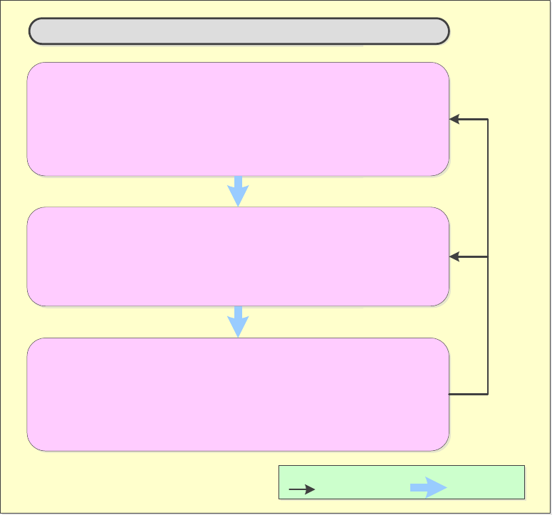
Handbook on Supply and Use Tables and Input-Output Tables with Extensions and Applications
449
Figure 13.3 Key feedback loops in producing and balancing
the PSUTs and environmental extended IOTs
13.67 In practice, the PSUTs will be compiled using the final balanced SUTs as a starting point.
The option for feedback to the SUTs, while it is then limited to the year or periods in question until
the next revision cycle, is still very useful. Any inconsistencies detected in balancing the PSUTs
may be used as additional information to guide the compilation and balancing of the next revision
of the affected SUTs. In some countries, this may have to wait for the next benchmark revision
year.
D. Environmental extended IOTs
13.68 The EE-IOTs are integrated datasets that combine information from standard monetary
IOTs and information on environmental flows, such as flows of natural inputs and residuals which
are measured in physical units. This section focuses on two types of EE-IOTs, namely the single
region IOTs and the hybrid IOTs. Reference to the multi-region IOTs will be made in this chapter
and expanded in chapter 17. The intent of this section is to introduce the main types of EE-IOTs,
SUTs at purchasers’ prices, basic prices, valuation matrices both in current prices
and previous years’ prices
• Population SUTs at purchasers’ prices
• Compile valuation prices
• Compile SUTs at basic prices
• Compile IOTs
Key phases
Compilation of Physical SUTs and Physical IOTs / EE-IOTs
• Collect price data (levels)
• Collect physical data (where applicable)
• Compile SUTs in physical terms (PSUTs)
• Compile IOTs in physical terms (PIOTs / EE-IOTs)
Validation, reconciliation and balancing
• Check key identities in physical terms
• Check plausibility of movements in physical terms
• Reconcile inconsistencies in physical terms
• Feedback/amendments from PSUTs/PIOTs/EE-IOTs to SUTs and/or IOTs
• Documentation
Key
Feedback loops Process flows

Handbook on Supply and Use Tables and Input-Output Tables with Extensions and Applications
450
to show key parts of their compilation, and to discuss some of the measurement issues associated
with them.
1. Single region IOTs
13.69 The single region IOTs consist of monetary IOTs extended to include environmental flows
in physical units. These tables are called “single region” tables as they are compiled for a single
territory (which can be either a country or a group of countries) and where the category “rest of
the world” includes all other territories or countries. This is in contrast with multi-region IOTs,
where the tables consist of sets of IOTs for more than one country and are combined in such a way
that intra-country relationships are explicitly identified. Chapter 17 of this Handbook elaborates
on multi-region IOTs.
13.70 Table 13.6 shows a simplified version of single region IOTs. It gives a detailed description
of domestic production processes and transactions within a single country (or region). An IOT is
usually structured as a product-by-product table or and industry-by-industry table. Table 13.6
shows an industry-by-industry table of industries. The rows show the outputs of an industry,
while the columns provide information about the inputs required in the production process of an
industry.
Table 13.6 Single region IOT with environmental data
Data in monetary terms
Industries
Final use
Total output
1
…
j
Final
consumption
Gross capital
formation
Exports
Industries
1
…
Z
C f e q+m
Value added
Total inputs
Data in physical (non-monetary) terms
Natural inputs /
residuals
r
tot
Notations:
• : Matrix of intermediate consumption ( by matrix)
• : Final consumption
• : Gross capital formation
• : Exports
Handbook on Supply and Use Tables and Input-Output Tables with Extensions and Applications
451
• : Value added
• : outputs of domestic industries
• : denotes the use of imported goods and services
• : Environmental flows (i.e. natural inputs or residual flows) taken from SEEA
• subscript denotes industry
• subscript denotes totals.
13.71 The output of the industries is the sum of intermediate consumption () (which is a by
matrix) and final use categories such as final consumption (), gross capital formation ()
(including changes in inventories), and exports (). It should be noted that, for all these categories,
this is the sum of domestically produced goods and services and imported products, namely =
+
, =
+
, =
+
, =
+
(subscript denotes the use of domestically
produced inputs and the use of imported goods and services). The inputs for each domestic
industry comprise the intermediate inputs () and value added categories (). Since the inputs into
an industry must equal the outputs, the column sums are thus equal to the outputs () of domestic
industries, while the row sums are equal to domestic output plus the imported products (+ ).
All the variables with the subscript are vectors that show the totals for those respective row or
columns.
13.72 The intermediate input matrix, , of IOTs is therefore a square matrix (in other words, it
contains the same number of rows and columns).
13.73 The IOT is then augmented with environmental data by industry (denoted by the vector
in Table 13.6), which may be taken from the relevant SEEA accounts. In most applications these
data relate to flows of natural inputs and residuals. The conceptual foundation for environmental
extensions to SNA-based IOTs, represented by the EE-IOTs, is described in the System of
Environmental-Economic Accounting 2012 – Applications and Extensions (United Nations,
European Commission, FAO, IMF, OECD and World Bank, 2017).
13.74 Having PSUTs available greatly facilitates the compilation of EE-IOTs, as the
environmental information is already organized into an accounting framework consistent with the
framework of the IOTs in terms of concepts, definitions and classifications. Extending the
monetary IOTs with available environmental statistics, however, and adjusted when necessary, for
the concepts and classifications of the SEEA, may be a starting point toward the compilation of
environmental-economic accounts in countries, starting with the implementation of the SEEA.
13.75 IOTs can be constructed as industry-by-industry or product-by-product tables. When a
product-by-product based structure is used for IOTs, adjustments to the environmental data are
necessary, since data on environmental flows are most commonly collected and classified by

Handbook on Supply and Use Tables and Input-Output Tables with Extensions and Applications
452
industry. The adjustment of environmental flow data in terms of industries and products will also
arise when SUTs form the basis for the representation of flows within the economy. SUTs are
generally structured with columns representing industries and rows representing products, with
substantially more products than industries. Examples of EE-SUTs are emerging in the literature
and may benefit from some analysis since they provide additional detail by product.
2. Hybrid IOTs
13.76 Hybrid IOTs consist of IOTs augmented with data in physical units for the input and output
of selected industries. Table 13.7 shows a hybrid IOT where data for the industry (shaded area
in Table 13.7) are also measured in physical terms. Many studies, for example, have analysed
energy using IOTs where the output of the energy industries is measured in gigajoules or another
energy unit. The source data from this type of data could, for example, be based on the PSUTs for
energy. Note that because the columns contain a mix of entries in different units (some monetary
and some physical), it is not possible to aggregate entries within a column. Summation across each
row is, however, possible.
Table 13.7 Single region IOT in hybrid units
Industries
Final use
Total output
1
…
J
Final
consumption
Gross capital
formation
Exports
Industries
1
…
Z
C F e q+m
J
J
(physical
units)
Value added
v
13.77 For environmental analysis, it remains relevant to extend the hybrid IOTs using
information on flows of natural inputs and residuals, as in the case of the single region IOTs. The
advantage of using physical units within the core IOTs is that, in many cases, this provides a better
description of the technological relationships for industries that have a reasonably large share of
physical rather than service-based flows. Hence, when applying the analytical techniques, there is
likely to be a better estimation of the direct and indirect environmental pressures across the
economy. It is important to note that the mathematical specifications of the input-out model apply,
irrespective of the units of the rows of the hybrid IOTs. The details of these types of models for
energy are provided in chapter 9 of Miller and Blair (2009).
13.78 This type of EE-IOTs incorporates elements of life-cycle analysis and process analysis
since it is possible to reflect the chain of flows between economic units in physical terms in the
context of an economy wide set of flows.

Handbook on Supply and Use Tables and Input-Output Tables with Extensions and Applications
453
E. Compilation of EE-IOTs
13.79 The compilation of the EE-IOTs, in particular single region IOTs, consists of two parts:
i. Monetary IOTs (upper block of Table 13.6)
ii. Environmental data by industry. In most applications these data relate to flows of natural
inputs and residuals (lower block of Table 13.6)
Table 13.8 Industry-by -industry IOTs (upper block of Table 13.6)
Data in monetary terms
Industries
Final use
Total output
1
…
j
Final
consumption
Gross capital
formation
Exports
Industries
1
…
Z
c f e q+m
j
Value added
v
Total inputs
q
c
tot
f
tot
e
tot
13.80 The monetary IOTs (Table 13.8) are derived from the SUTs following the steps described
in the previous chapters of this Handbook.
Table 13.9 Environmental data by industry (lower block of Table 13.6)
Data in physical (non-monetary) terms
Industries
Final demand
Total output
1
…
J
Final
consumption
Gross capital
formation
Exports
Natural inputs /
residuals
r r
tot
13.81 The environmental data are organized by industry in Table 13.9. Examples of such data
items are resource use and emission per industry. In most applications these data relate to flows of
natural and residual inputs. Details of the common national data sources and relevant materials for
each SEEA component of accounts of physical flows may be found in tables 13.4 and 13.5 above.
13.82 The environmental data do not necessarily have to be derived from PSUTs. Usually, the
information on environmental flows, the basic data, will not be strictly aligned with the
measurement boundaries of the SEEA. Care should therefore be taken to record appropriately,
with adjustment as necessary, entries for purchases made abroad by tourists and for re-exports.
Careful attention should also be paid to the general issue of recording data on a residence basis
rather than a territory basis. Having balanced PSUTs behind the information in table 13.9 helps to
Handbook on Supply and Use Tables and Input-Output Tables with Extensions and Applications
454
guarantee the reliability of the information and the consistency between monetary and physical
data (ensured by the balancing feedback loops).
13.83 In addition to the materials listed in Box 13.1, a number of databases have been developed
that incorporate physical flows and environmental information. They require the integration of
data from various data domains as envisaged in the EE-IOTs: the 2012 WIOD (Dietzenbacher and
others, 2013, and Timmer, 2012) and the projects on an environmental accounting framework
using externality data and input-output tools for policy analysis (EXIOPOL) and compiling and
refining of economic and environmental accounts (CREEA) funded by the European Union.
13.84 There are a number of measurement issues that should be borne in mind when compiling
the EE-IOTs. In the 2008 SNA, imports and exports are defined on the basis of ownership rather
than physical flows. In physical terms, however, a difference in the recording of some flows of
products (for example, goods sent abroad for processing) may need to be taken into account (see
chapter 3 of the SEEA Central Framework for more details of the treatment in physical terms).
Consequently, analysis seeking to use information in both monetary and physical terms may
require adjustment to either data set to ensure an alignment in the treatment of certain flows.
13.85 Basic environmental statistics may not be in strict alignment with the measurement
boundaries of the SEEA. Care should therefore be taken to record, and adjust if necessary, in an
appropriate manner, entries for purchases made abroad by tourists, re-exports and the general issue
of recording data on a residence basis rather than on that of territory (further details may be found
in section 3.3 of the SEEA 2012– Central Framework).
F. Country examples
13.86 This section presents two country examples in the compilation of PSUTs: Denmark and
the Netherlands. An example of the compilation of EE-IOTs may be found in chapter 19,
section D.
1. Danish PSUTs
13.87 In Statistics Denmark, the compilation of SUTs is not just an integral part, it even serves
as the backbone of the annual Danish national accounts in current prices and in previous years’
prices. Every year, as part of the final annual national accounts, the SUTs are constructed using a
classification level including 117 industries, 135 groups of final use, and approximately 2,350
products, of which approximately 1,800 may be characterized as goods (physical products).
13.88 The PSUTs follow as closely as possible, where applicable, the layout, classifications and
definitions, and methods used for the Danish SUTs and IOTs. Furthermore, in order to ensure
correspondence between the SUTs and IOTs, on the one hand, and the PSUTs, on the other, and
to speed up the data handling and construction of the tables, the information technology system
Handbook on Supply and Use Tables and Input-Output Tables with Extensions and Applications
455
and database used for balancing and preparing the monetary tables have been extended to include
the physical information.
13.89 The accounts for waste and water are produced independently of the SUTs. The monetary
and physical energy accounts are produced as part of the SUTs process and enter directly into the
national accounts SUTs and the PSUTs, respectively. The emissions accounts are subsequently
based on PSUTs for energy, with some additions for non-energy-related air emissions. It should
be noted that Statistics Denmark also produces physical IOTs after the PSUTs have been produced
and, in this process, all the physical accounts fit directly into an environmental extended IOTs
framework.
13.90 The PSUTs are integrated with, and build partly on, the existing Danish economy-wide
material flows accounts, energy and air emission accounts.
13.91 The economy-wide material flows accounts are based on information from resource
extraction statistics, fisheries statistics, agricultural statistics and foreign trade statistics. All
information is available in tons.
13.92 The system of PSUTs is constructed as a further layer to the SUTs. This means that the
same classifications of industries and products are used for the physical flows. For the final uses,
a slightly different classification is used. Thus, the physical flows are less relevant for some
consumption groups while, on the other hand, it may be more appropriate to classify households’
final consumption expenditures according to whether the consumption involves durable goods or
not.
13.93 For the Danish PSUTs, more than 100 types of natural resources (various types of biomass
and minerals) and 40 types of residuals (types of solid waste and air emissions) were added to the
classification of materials and products, giving a total of approximately 2,000 items along the
materials and products dimension of the system.
13.94 Figure 13.4 shows the complete system of monetary and physical flow data, including
monetary data on products, and physical data on natural inputs, products and residuals. The top
layers are monetary data, including, on the supply side, basic prices only and, on the use side, basic
prices, trade margins, taxes, and purchasers’ prices. The bottom (light blue) layer is physical data
measured in tons. For products, there is a one-to-one correspondence between the monetary data
and the physical data.
13.95 In front of the physical layer of products, as shown in figure 13.4, the data for natural
resources are added. The environment is added as the supplier of natural resources, while the
industries (intermediate consumption) are the only users.
13.96 The residuals are also added to the layer of products. The supply comes from industries
and households. It should be noted that, unlike in the SUTs, the households are now also

Handbook on Supply and Use Tables and Input-Output Tables with Extensions and Applications
456
represented on the supply side, since they also generate residuals. The users of residuals are both
industries and the environment. Residuals such as waste for incineration go into the waste
treatment industry, while air emissions go into the environment.
13.97 In practice, all monetary and physical data illustrated in Figure 13.4 are stored and managed
in a file using a common system of transaction codes and classifications. Each flow is identified
first by a product code for the natural resource, product or residual. This code is followed by a
transaction code (covering type, origin or destination), classification (the specific industry, and so
forth) and then the data for basic prices, wholesale and retail margins, taxes (excluding VAT) less
subsidies on products, VAT, purchasers’ prices and finally the quantity (in tons).
13.98 The Danish energy accounts present the supply and use of 40 types of energy products.
The supply and use of products are broken down by domestic industries, households, imports and
exports and other parameters. The Danish energy accounts are made up using various measuring
units: monetary units (Danish kroner), natural physical units (tons, cubic metres, and so forth) and
energy units (petajoules). Tons are used for the purpose of the PSUTs.
Figure 13.4 Danish SUTs framework extended with physical flows
FINAL USE
INDUSTRIES
Purchasers' prices
VALUATION
Intermediates
Non-deductible VAT
Other net taxes on products
NATURE
Trade marggins
Basic prices
QUANTITIES (tons)
IMPORTS
INDUSTRIES
Flow to environment
Exports
Change in inventories
Gross fixed capital fomation
PRODUCTS
Consumption of government
Consumption of households
Industries LEGEND
Flow from environment (Nature as supplier)
Gross capital formation (Accumulation)
Consumption of households
Taxes less subsidies on products
Valuation matrices
RESIDUALS Trade and tranport margins
Imports
NATURAL INPUTS
Industries Quantities (tons)
BALANCING ITEM
SUPPLY TABLE
Values at purchasers'
prices
Values at basic prices
USE TABLE
Intermediates at
purchasers' prices
Value added at
basic prices
Final use at
purchasers' prices
Domstic production
at basic prices
Handbook on Supply and Use Tables and Input-Output Tables with Extensions and Applications
457
13.99 Data on energy-related air emissions of carbon and sulphur are drawn from the Danish air
emission accounts. The air emission accounts show the energy-related and other types of air
emissions of various substances from industries and households. The CO
2
and SO
2
air emissions
are converted into carbon and sulphur, based on the molecule weights. This procedure is used since
the oxygen used for the combustion of energy is not included on the input side of the PSUTs
system.
13.100 In addition to the economic-environmental accounts, a number of other data sources are
used:
• Waste statistics (physical data) broken down by waste fractions
• Water statistics (physical data)
• Foreign trade statistics
• Production statistics (physical and monetary data)
• Agricultural, forestry and fishery statistics (physical data)
• SUTs from the national accounts (monetary data)
• Assumptions used in transforming the SUTs to IOTs
13.101 As a general rule, water is not included in the Danish PSUTs. In order to balance inputs
and outputs, however, it is necessary to account for the inclusion of water in some products (for
example, beverages), on the input side and the evaporation of water from products (for example
from slaughtered animals) on the output side. Water supplied for production purposes in
agriculture, horticulture, forestry and fishery is implicitly included when calculating the input of
natural resources from the harvested biomass weight. Information on the quantities of water added
to products is also obtained by including existing structural information, and by estimations carried
out during the general balancing process.
13.102 The foreign trade statistics include very detailed data on the imports and exports of
products. The information is available in both monetary values and quantities measured in tons,
and sometimes also additional physical units (such as cubic metres).
13.103 The compilation of domestic production in tons broken down by industries is primarily
based on the production statistics of Statistics Denmark for the manufacturing industries while
agricultural, forestry and fishery statistics are used for the corresponding primary industries. In the
case of a number of items in the product balances, there is no information in the product statistics
on the weight in tons, and this is therefore estimated indirectly. In those cases where alternative
quantitative information has been given in, for example, cubic metres or pieces, a conversion is
made from such conversion factors as specific gravity or weight per piece. In other cases, the

Handbook on Supply and Use Tables and Input-Output Tables with Extensions and Applications
458
quantities are estimated on the basis of value and corresponding unit volume price. As price and
quantitative information is available for exports in almost all product balances based on the foreign
trade statistics, the unit volume prices are typically calculated on the basis of the proportionality
between the basic price and the weight of the exported item.
13.104 Thus, all cells for resource flows, all cells for imports and exports and domestic production
and most cells for residual flows can initially be filled out by using the physical data sources as
described above. By contrast, with a few exceptions, it is not possible to fill out the various
domestic uses of products from the basic data. Those exceptions include agricultural products and
energy products, where reliable data on the uses can be found in many cases.
13.105 Figure 13.5 shows the various stages in transforming basic data and statistics into PSUTs.
Figure 13.5 From source data to PSUTs
Balancing the PSUTs
13.106 It is a fundamental principle of accounting that the flow of materials (natural resources,
products and residuals) into a single industry or into households must be precisely matched by a
corresponding accumulation or flow from the industry or household group.
Handbook on Supply and Use Tables and Input-Output Tables with Extensions and Applications
459
13.107 Although the initial filling out and estimations ensure that, for each product, the total
supply equals total use, there is no guarantee that the material balance for the industries and
households in question actually exists.
13.108 For each of the 117 industries and the households represented in the PSUTs, it is therefore
necessary to adjust the inputs or outputs until a complete balance between material inputs and
outputs (including accumulation) is obtained.
13.109 The balancing is undertaken, among other factors, in the light of information on the
technical production conditions in the industries, obtained from different technical reports and
additional statistical information. In addition to this, it is necessary, in a very large number of
cases, to use estimates and common-sense considerations.
13.110 The reconciliation of the inputs and outputs in the Danish PSUTs system is carried out for
11 subgroups of materials (natural resources, products and residuals) corresponding to relatively
similar or coherent groups of materials, for which there is an apparent connection between inputs
and outputs. The groups are: energy, agricultural products, glass, metallic minerals, construction
minerals, plastic, wood and paper, rubber, chemical products and fertilizers, lubricants and oil
waste, and other materials.
13.111 The 11 individual sub-P SUT systems are reconciled before a final reconciliation of the
total PSUTs takes place, because it is easier and more logical to focus on inputs and outputs of
products that are physically connected through the production processes. For example, when the
sub-physical SUTs for energy are reviewed, these will include the input flows of natural gas, crude
oil and biomass used for energy production, all energy products and energy-related residuals, while
all other products are excluded. The energy-related residual flows comprise air emissions of carbon
and sulphur, other energy-related air emissions and solid waste of fly ash and, for instance,
desulphurization products, and others.
13.112 For other groups besides energy, there are in practice certain links between them, for
example, inputs of chemical products and fertilizers are used in relation to the production of animal
and crop products. The existence of these links between the different groups means that it is not
possible to make a complete balance within one single group, and instead an interim balancing
item is introduced for each subgroup in the system (except for energy). When positive for an
industry, this artificial residual represents a net input of materials belonging to other groups in the
industry. When negative, this means that the industry delivers products of the specific material
type to be used as inputs for the production of products of another material type.
13.113 If the balancing of the 11 subgroups is carried out with complete accuracy, the individual
balancing items will cancel each other out when they are added up. In practice this is not the case,
since the balancing items will also include uncertainties and inconsistencies introduced during the
initial phases and balancing processes. Accordingly, it is necessary to make a final balancing to
ensure that the artificial residuals sum to zero.

Handbook on Supply and Use Tables and Input-Output Tables with Extensions and Applications
460
13.114 Table 13.10 shows a numerical example of PSUTs for Denmark for the year 2009 (it should
be noted that the data in Table 13.10 were preliminary). The supply table shows that 104.9 million
tons of natural inputs were extracted from the environment in Denmark. All these inputs were used
by Danish industries. In all, 295.5 million tons of products were supplied, of which 232.6 million
and 62.9 million tons were Danish output and imports, respectively. The 295.5 million tons of
products were used as follows: 176.4 million tons were used for intermediate consumption by
industries; 18.9 million tons were used in household consumption; 62.0 million tons were used for
gross capital formation; and 38.3 million tons were exported. Industries generated 48.7 million
tons of residuals and households 18.9 million tons of residuals.
Table 13.10 PSUTs in Denmark
13.115 The use table shows that all these residuals go into the environment. Following the SEEA
Central Framework conventions, residuals that are sent to controlled landfills should be recorded
as accumulation in the economy, but for these simplified Danish SUTs they are not recorded as
such.
13.116 Table 13.10 also shows that the basic bookkeeping identities covered above are all fulfilled.
For accumulation, rest of the world and environment, there is no balance between supply and use
of products, but when all three items are considered together, the total supply equals total use. This
indicates that, in 2009, Danish imports exceeded Danish exports and that the extraction of natural
inputs from the environment exceeded the amount of residuals that were returned to the
1000 tons
Industries Housholds
Govern-
ment
Accu-
mulation
Rest of the
world
Environ-
ment
Total supply
Natural inputs 104 965 104 965
Products 232 603 62 901 295 505
Residuals 48 732 18 867 67 600
Total 281 336 18 867 62 901 104 965 468 069
1000 tons
Industries Housholds
Govern-
ment
Accu-
mulation
Rest of the
world
Environ-
ment
Total supply
Natural inputs 104 965 104 965
Products 176 370 18 867 61 958 38 309 295 505
Residuals 67 600 67 600
Total 281 335 18 867 61 958 38 309 67 600 468 069
Denmark 2009 = Grey cells are null by definition.
Physical supply table
Physical use table
Handbook on Supply and Use Tables and Input-Output Tables with Extensions and Applications
461
environment. In this way the exchange of materials between the Danish economy and the rest of
the world, plus nature, showed a surplus of 62.0 million tons of material. This amount is exactly
equal to the accumulation of materials in the economy as shown in the column for accumulation.
2. PSUTs in the Netherlands
13.117 The PSUTs compiled by Statistics Netherlands are fully in line with the standards set out
by SEEA. The starting point for the PSUTs is the balanced SUTs, compiled as part of the national
accounts. While the physical flows have a monetary value, the flows without a monetary value are
added on (for example natural inputs, waste and emissions). The integration of all physical flows
in the PSUTs generates a consistent and coherent set of data which are also consistent with the
monetary information contained in the monetary SUTs of the SNA. As a consequence, such
economic variables as labour and GVA can be analysed in combination with the physical data
shown in the PSUTs. Statistics Netherlands regularly compiles SUTs, IOTs and PSUTs, but not
physical IOTs.
(a) Structure of the PSUTs for the Netherlands
13.118 The PSUTs follow as closely as possible the structure and classifications of the SUTs. One
important difference between the SUTs and PSUTs is that the PSUTs also include the physical
flows that do not have a monetary value. In the supply table, air emissions and waste are recorded
(the former under the heading balancing item in the example below). In the use table, recycled
waste and extraction from the environment are taken into account. In addition, a balancing item is
introduced in order to achieve the material balance at the industry level, which consists of items
such as emissions other than carbon dioxide, the supply and use of water, and others.
13.119 Table 13.11 shows an example of the SUTs for the Netherlands for 2010 and Table 13.12
shows the corresponding PSUTs for the same year.

Handbook on Supply and Use Tables and Input-Output Tables with Extensions and Applications
462
Table 13.11 SUTs for the Netherlands, 2010
Netherlands 2010
Supply table at basic prices
Million Euro
Agriculture
Manufacturing
and
construction
Services
Total
(1) (2)
(3) (4) (5) (6)
Agriculture (1) 25 299
153
41 25 493 13 900 39 393
Manufacturing
(2) 1 230
282 553 35 780 319 563 301 843 621 406
Construction
(3) 70 84 922
4 676
89 668 1 521
91 189
Trade, transport and
communication
(4) 565
15 375
222 573 238 513
20 319 258 832
Finance and business services (5) 477 7 803
274 997
283 277 50 908 334 185
Other services (6) 312
2 531
219 567 222 410 16 366 238 776
Total
(7) 27 953
393 337 757 634
1 178 924 404 857
1 583 781
CIF/FOB adjustments on imports
(8) - 3 272
- 3 272
Direct purchases abroad by
residents
(9)
Total
(10) 27 953
393 337 757 634
1 178 924
401 585 1 580 509
Use table at basic prices
Million Euro
Total
Households NPISH
General
government
(1) (2) (3) (4) (5) (6) (7) (8) (9) (10)
(11) (12)
Agriculture
(1) 4 679 13 686 1 152 19 517 2 461 161 168 17 086 19 876
39 393
Manufacturing
(2) 7 921 153 180 47 758 208 859 54 468
5 373 39 357 3 775 309 574 412 547 621 406
Construction
(3) 292
23 573 17 370 41 235 399 522 46 786 2 247 49 954
91 189
Trade, transport and
communication
(4) 1 790 31 077 73 293
106 160
62 054 860 3 725 10 673 77
75 283
152 672 258 832
Finance and business services (5) 2 052
41 219 152 096
195 367
74 771 5 3 546
13 442
47 054
138 818 334 185
Other services
(6) 169 3 429 20 925 24 523 50 518
4 451 153 957 461
285
4 581
214 253 238 776
Total at basic prices
(7) 16 903
266 164 312 594 595 661 244 671 5 316
167 123 110 880 4 305 455 825 988 120
1 583 781
Taxes less subsidies on products
(8)
222 1 493 13 791
15 506 32 523 109 13 769 3
1 845 48 249 63 755
Total
(9) 17 125 267 657 326 385 611 167
277 194 5 316 167 232
124 649 4 308 457 670 1 036 369
1 647 536
CIF/FOB adjustments on exports
(10)
- 3 272
- 3 272 - 3 272
Direct purchases abroad by
residents
(11)
Purchases on the domestic territory
by non-residents
(12)
Total at purchasers’ prices
(13) 17 125 267 657 326 385 611 167 277 194 5 316 167 232 124 649 4 308 454 398 1 033 097 1 644 264
Compensation of employees
(14) 2 603 59 807 248 061
310 471
310 471
Other taxes less subsidies on
production
(15) - 537
- 106 - 337 - 980 - 980
Consumption of fixed capital
(16) 3 660 20 186 83 136 106 982 106 982
Net operating surplus
(17) 5 102 45 793 100 389 151 284
151 284
GVA (18) 10 828 125 680 431 249 567 757 567 757
Total
(19) 27 953 393 337 757 634 1 178 924 277 194
5 316 167 232 124 649 4 308 454 398 1 033 097 2 212 021
= Grey cells are null by definition.
GVA
INDUSTRIES
FINAL USE
Total use at
basic prices
PRODUCTS
Gross fixed
capital
formation
Exports
Changes in
inventories
INDUSTRIES
Imports
Total
supply at
basic
prices
PRODUCTS
Agriculture
Manufacturing
and
construction
Services
Total
Final consumption expenditure

Handbook on Supply and Use Tables and Input-Output Tables with Extensions and Applications
463
Table 13.12 PSUTs for the Netherlands, 2010
Netherlands 2010
Transformation from SUTs to PSUTs
13.120 The starting point for the compilation of PSUTs (in kilograms) is the balanced SUTs valued
at basic prices. In addition to the data used for the SUTs, there are several data sources available
covering prices and quantities. The most important sources are:
• Foreign trade statistics
• Data on output of manufacturing
• Data on intermediate use from business statistics (limited)
• Scanner data from supermarkets
• Price information from branch organizations and dedicated research institutes (mainly with
regard to agriculture)
Physical supply table
Million kilogram
Agriculture
Manufacturing
and
construction
Services
Total
(1)
(2) (3) (4) (5) (6) (7) (8) (9)
Agriculture
(1)
43 592 31 43 623 26 779 70 402
Manufacturing
(2) 182 334 216 16 345 350 743 328 027 678 770
Construction
(3)
Trade, transport and
communication
(4)
Finance and business
services
(5)
Other services
(6)
Total
(7) 43 774 334 247 16 345 394 366 354 806 749 172
Waste
(8) 74 596 50 944 5 136 130 676 9 297 6 059 15 350 161 382
Extraction
(9) 143 679 143 679
Balancing item
(10) 75 143 258 891 88 265 422 299 85 219 282 455 789 973
Total
(11) 193 513 644 082 109 746 947 341 94 516 6 059 370 156 426 134 1 844 206
Physical use table
Million kilogram
Agriculture
Manufacturing
and
construction
Services Total
(1) (2) (3) (4) (5) (6) (7) (8) (9) (10)
Agriculture
(1) 5 957 41 879 1 875 49 711 2 437 216 10 197 7 841 70 402
Manufacturing
(2) 17 955 292 152 47 582 357 689 31 280 7 573 184 069 98 159 678 770
Construction
(3)
Trade, transport and
communication
(4)
Finance and business
services
(5)
Other services
(6)
Total
(7) 23 912 334 031 49 457 407 400 33 717 7 789 194 266 106 000 749 172
Waste
(8)
76 602 68 068 144 670 1 495 15 217 161 382
Extraction
(9) 38 778 101 095 3 806 143 679 143 679
Balancing item
(10) 54 221 140 888 56 483 251 592 60 799 101 610 375 972 789 973
Total
(11) 193 513 644 082 109 746 947 341 94 516 110 894 209 483 106 000 375 972 1 844 206
= Grey cells are null by definition.
Flow to
environment
Total
PRODUCTS
Total
PRODUCTS
INDUSTRIES
Households
Accumulation
Exports
INDUSTRIES
Households
Accumulation
Imports
Flow from
environment
Re-exports
Handbook on Supply and Use Tables and Input-Output Tables with Extensions and Applications
464
• Quantity data on energy and energy-related products from the energy accounts
13.121 Following the approach of Konijn, de Boer and van Dalen (1995), the initial estimates for
the physical use of products are compiled by applying import prices to the monetary use table. The
physical supply is initially estimated by applying export prices to the monetary supply table. The
justification for this is that a large share of the domestic production of goods is exported, while a
large share of the use of goods is imported.
13.122 If specific data are available, these initial estimates are overruled in the next step. The
business statistics dedicated to the composition of output provide information on prices and
quantities of the supply of goods for manufacturing at the three-digit or four-digit level of NACE
Revision 2. This information is especially useful in cases where the products are not homogeneous,
leading to a difference in prices among industries. It may also happen that differences in quality
between products lead to differences in prices. For example, meat produced by slaughterhouses
will probably be of a different quality than meat produced by the food-processing industry. As a
consequence, there will be a difference in price levels between the meat products emanating from
these two industries.
13.123 For a limited number of industries, price information for the intermediate inputs is available
and this can be used to overrule the initial physical estimates based on import prices. Additional
price information collected by branch organizations and research institutes is also used. The most
important examples cover price data for agricultural products; together with harvest estimates,
these provide a sound base for estimating the physical flows in this area.
13.124 Scanner data provided by supermarkets are a valuable source of information for the
transformation of the whole or part of the consumption of households into physical units.
13.125 In addition to the price information, the physical information observed is used in compiling
the PSUTs. This mainly covers the data on agriculture and energy (crude oil, fuel, natural gas,
electricity, and other forms of energy). Data on energy are derived from energy accounts.
13.126 Through the application of this information on balanced SUTs, PSUTs for all relevant
products may be prepared, even though these PSUTs are not balanced.
13.127 In addition to the physical flows for supply and use of products, the physical flows for
materials not having a monetary value are included. These mainly concern flows between the
economy and the environment, such as air emissions, extraction of natural resources, the input of
oxygen in combustion processes and waste. Adding these flows will make it possible to analyse
the balance of physical input and physical output at the industry level. Emission and waste statistics
are the main sources for making initial estimates for these physical flows. The items mentioned
only cover parts of the non-monetary flows; the extraction of water by the production of beverages,
for example, is missing. When the PSUTs are balanced, the adjustments for these missing items
are made.
Handbook on Supply and Use Tables and Input-Output Tables with Extensions and Applications
465
Accumulation
13.128 On the supply side the material flows are incorporated, resulting from the reduction of
physical stocks of products. Examples include the growing availability of physical residuals due
to the demolition of machines and buildings and air emissions from controlled landfills. A
distinction is made between types of waste, such as the waste resulting from a production process
and the waste resulting from scrap of capital goods, for example.
13.129 On the use side, the additions to the capital stock (gross fixed capital formation, both
monetary and physical) and the accumulation of waste in landfills are taken into account. As the
estimates of the accumulation part of the PSUTs are not straightforward, they form a less reliable
part of the PSUTs.
Balancing the PSUTs
13.130 The initial estimates of the PSUTs are not balanced – neither at product level (rows) nor at
industry level (columns). There are several causes underlying the inconsistencies between the
supply and use of products in the PSUTs. As observed previously, products which are not
homogeneous can give rise to inconsistencies because the prices may differ significantly between
the various producing and using industries. The assumption that output is mainly exported and
intermediate use is mainly imported is not always valid. When significant parts of domestic output
are used domestically, inconsistencies are likely to appear. Lastly, some of the source data could
be inaccurate.
13.131 The balancing of the PSUTs has three steps:
• Detection and balancing of major inconsistencies at the product level
• Detection and balancing of major discrepancies between input and output in physical terms
by industry
• Automated balancing of minor inconsistencies
13.132 During the balancing at the product level, major inconsistencies between supply and use
on a product level are resolved by analysing the link between the physical volumes of outputs and
the physical volumes of inputs (for example the number of cattle entering the slaughterhouses and
the volume of meat produced). In this stage, the input from the branch specialists is used in judging
the plausibility of the results.
13.133 In the balancing of the input and output in physical terms by industry, the material flows
to and from the environment are taken into account. In the supply table, the carbon dioxide and
water emissions in combustion processes are taken into account. In the use table, the oxygen
necessary for combustion is recorded. A specific estimate is made for nitrogen (N
2
) extracted from
the air in producing ammonia. Estimates for the other emissions to the air or water are not made
Handbook on Supply and Use Tables and Input-Output Tables with Extensions and Applications
466
because they are relatively small compared to carbon dioxide emissions. The above mentioned
items, excluding carbon dioxide emissions resulting from combustion, are recorded as part of the
balancing item with the industries in the PSUTs.
13.134 In addition to the above mentioned flows, the balancing item consists of the water content
of products. The production of beverages has a relatively low intermediate input of raw materials
because the main input is water, which is extracted from the environment.
13.135 The opposite can also happen in that the water content is reduced in the production process.
In the PSUTs for the Netherlands, separate estimates are made for the water content of products,
and, in this way, the estimates by industry are made on whether the balance of the water is supplied
to or extracted from the environment. This information is used to judge the plausibility of the
balancing items by industry.
13.136 In many cases, a balancing item is necessary for those types of industries where services
are produced but where a considerable proportion of inputs consist of goods, for example
restaurants and pubs. A meal in a restaurant is recorded as a service, while the inputs are goods
and services.
13.137 In the construction industry, the physical estimate of output is relatively low because no
direct estimate is made of the physical value of dwellings, buildings, roads, etc. as a consequence
of a lack of data. The physical output for construction is accounted for in the balancing item in the
supply table.
13.138 As a consequence, the theoretical contents of the balancing item may vary greatly between
industries.
13.139 The remaining minor inconsistencies are balanced using an automated balancing procedure
similar to the approach used for balancing the SUTs, as covered in chapter 11 of this Handbook.
Handbook on Supply and Use Tables and Input-Output Tables with Extensions and Applications
467
Chapter 14. Supply and use tables and quarterly national accounts
A. Introduction
14.1 The previous chapters of this Handbook focused primarily on the compilation of annual
SUTs. SUTs can also play an important role, however, in the compilation of quarterly national
accounts, by ensuring the consistency and coherence of the estimation of the accounts.
14.2 Although the ideal scenario is for SUTs to be compiled and published on a quarterly basis
and benchmarked with the annual SUTs, this is often difficult to achieve, owing, for example, to
data unavailability, lack of human and financial resources and time constrains. Nonetheless,
quarterly SUTs provide a key tool for the compilation of quarterly national accounts or as a
minimum a validation tool of such accounts.
14.3 For both quarterly and annual SUTs, an integrated approach to balancing in current prices
and in volume terms and also at basic prices and at purchasers’ prices will ensure a high degree of
consistency and coherence.
14.4 The present chapter provides an overview of ways in which SUTs can be used to improve
the quarterly national accounts. Since there are various scenarios that can be used in practice, this
chapter focuses only on three main situations which represent the use of SUTs in various degrees
in the compilation of the quarterly national accounts.
14.5 A progressive approach could be implemented whereby the annual SUTs are first used to
improve the quarterly national accounts, then the quarterly supply and use of product-based models
are put in place to edit and validate the quarterly national accounts and, lastly, quarterly balanced
SUTs are compiled and published when appropriate data sources and validation processes are
developed.
14.6 Section B of this chapter provides a general overview of the quarterly national accounts
and the main differences between their compilation and that of annual national accounts, in respect
of data sources, revisions, timings, level of detail and other characteristics, and the issue of
benchmarking the quarterly national accounts with the annual national accounts. Section C
describes in more detail the uses of SUTs in the compilation of the quarterly national accounts.
Reference sources that provide additional detail include: Eurostat (2013b) Handbook on Quarterly
National Accounts and the IMF (2017) Quarterly National Accounts Manual.
Handbook on Supply and Use Tables and Input-Output Tables with Extensions and Applications
468
B. Quarterly national accounts
14.7 The quarterly national accounts constitute a system of integrated quarterly time series
coordinated through an accounting framework. The quarterly national accounts adopt the same
principles, definitions and structure as that applied in the annual national accounts. In principle,
the quarterly national accounts cover the entire sequence of accounts and balance sheets in the
SNA. In practice, the constraints of data availability, time, and resources mean that the quarterly
national accounts are usually less complete than their annual counterparts.
14.8 The main purpose of the quarterly national accounts is to provide a picture of current
economic developments much more quickly than the annual national accounts and more
comprehensive than those provided by individual short-term indicators. Thus, the quarterly
national accounts may be seen as positioned between the annual national accounts and specific
short-term indicators in many of these purposes. The quarterly national accounts are commonly
compiled by combining annual national account data with short-term source statistics and annual
national account estimates (for example, benchmarked to annual estimates).
14.9 In general, in the identification of sources and design of methods, the same principles apply
to both the annual and the quarterly national accounts. The quarterly national accounts data sources
are generally more limited, however, in detail and coverage than those available for the annual
national accounts because of issues of data availability, collection cost, and timeliness and this
may affect the level of detail of the quarterly national accounts. Some compilation issues that are
more pertinent to the compilation of either the short-term indicators or the quarterly national
accounts include:
• Monthly or quarterly type adjustments (for example, working days, trading days, moving
holidays, leap years, etc.)
• Seasonal adjustment (for example, handling annual sale periods, use of autoregressive
integrated moving average (ARIMA) models, trend cycle estimation)
• Quarterly chain-linked volume estimates
• Deriving estimates of quarterly variables consistent with annual benchmarks
• Smoothing
• Forecasting and nowcasting
14.10 In addition, the compilation of the quarterly national accounts is not to be considered in
isolation but as a consistent and coherent part of the annual national accounts process and part of
a time series. This will entail additional work in the compilation of the quarterly national accounts
to benchmark the quarterly national accounts with the annual national accounts, on the one side,
Handbook on Supply and Use Tables and Input-Output Tables with Extensions and Applications
469
and to revise previous quarters as more information becomes available, on the other. Issues with
the data sources and benchmarking are further considered below.
1. Data sources
14.11 Ideally, the same data sources used for the annual estimates of GDP should be used for the
quarterly estimates. This is often not possible, however, because the data are not available on a
quarterly basis (in other words, detailed breakdowns are not available) or less timely, and, when
they are available, the higher frequency data may be less accurate and reliable.
14.12 For example, the present practice in the United Kingdom for early GDP data releases is as
follows:
• First (preliminary) estimate of United Kingdom GDP is released some 25 days after the
quarter.
• Second estimate of the GDP is released some 55 days after the quarter.
• Third estimate of the GDP is released some 85 days after the quarter, together with the full
quarterly national accounts, balance of payments and the institutional sector non-financial
and financial accounts.
14.13 The first estimate of United Kingdom GDP contains a mix of collected data (for example,
data from business surveys and administrative data) and data based on forecasts and nowcasts to
complete the picture. Here the short-term indicators play a key role. The first estimate is heavily
based on the production (or output) approach to measuring GDP using proxies to estimate output
and an assumption that GVA moves in line with output in the short-term. At this stage, there are
very limited data underlying the expenditure approach to measuring GDP. With the move to the
second estimate and through to the third estimate, more and more data become available replacing
the earlier forecasts of missing data for both approaches. By the time the third estimate is produced,
there are also some data available for the income approach to measuring GDP.

Handbook on Supply and Use Tables and Input-Output Tables with Extensions and Applications
470
Figure 14.1 Quarterly GDP production (output) aggregate: data availability
and estimation in the United Kingdom
14.14 Figure 14.1 shows how the quarterly data underlying the production (output)-based
aggregate evolve over time, in which process the collected data replace early forecasts and
nowcasts of missing data. Similarly, Figure 14.2 shows how the underlying components of the
expenditure approach to measuring GDP evolve over time.

Handbook on Supply and Use Tables and Input-Output Tables with Extensions and Applications
471
Figure 14.2 Quarterly GDP expenditure components: data availability and estimation in
the United Kingdom
14.15 Many countries have monthly and quarterly surveys collecting a wide-range of economic
information but generally not with the same level of detail or coverage of the corresponding annual
surveys. Various totals may be collected but no breakdowns, for example, total turnover may be
collected but not with a product breakdown. Thus the structure of the last annual SUTs (preferably
in volume terms) or the last dataset collected helps to provide the ratios and percentages needed to
break down the totals to be carried forward in the compilation process prior to any quarterly
balancing process.
14.16 Similarly, administrative data, where available, can also be used in the quarterly national
accounts. Some administrative data, however, may not be timely enough for the quarterly national
accounts, such as, for example, labour costs or self-employment incomes.
14.17 The quarterly national accounts may therefore be less accurate than the more
comprehensive annual national accounts for a number of reasons, including the following:
• Less information is available on a quarterly basis than on an annual basis and there is more
reliance on proxy indicators.
• The basic quarterly statistics are often less robust than the annual equivalents (for example,
the annual data may be available through annual audited accounts).
• The sample sizes in the quarterly business surveys are smaller.
Handbook on Supply and Use Tables and Input-Output Tables with Extensions and Applications
472
• There are greater sample and non-sample errors in the data sources.
• Balancing is not completed through quarterly SUTs, whereas the SUTs framework may be
applied annually.
14.18 It is therefore important to have a framework that allows for the confrontation of the
different data sources and their reconciliation. The SUTs framework allows for the analysis and
reconciliation of data inconsistencies thanks to which a coherent picture is provided of GDP and
its components.
2. Data reconciliation, benchmarking and revisions
14.19 An important step in the compilation of the quarterly national accounts is the benchmarking
of these accounts with the annual national accounts when the latter become available. This is a
necessary step to ensure that the quarterly national accounts are consistent with the annual accounts
and with the short-term evolution of quarterly indicators. Benchmarking refers to the procedures
used to maintain consistency among the time series available at different frequencies (in this case,
annual and quarterly) for the same target variable.
14.20 The need to synchronize the implementation of major revisions including benchmarking
was briefly covered in chapter 11. These exercises should, in particular, be implemented, compiled
and balanced through a SUTs framework both in current prices and volume terms and also at basic
prices and at purchasers’ prices.
14.21 Since quarterly data sources are not of the same quality as the equivalent of the annual data
sources (for reasons already mentioned above, such as smaller survey samples, coverage, and
others), benchmarking usually consists of adjusting quarterly data to match annual (or
quinquennial) benchmarks. Once the quarterly national accounts have been benchmarked with the
annual national accounts, both the quarterly and the annual national accounts are consistent in the
sense that the annual accounts are the sum (or the average) of the quarterly accounts.
14.22 Before the benchmarking exercise is undertaken, a separate reconciliation exercise should
be considered, requiring dedicated resource and time. This involves reconciling the data from the
short-term and quarterly survey source and the annual source. For example, the annual growth rate
and current price level for, say, turnover, should be aligned. The same reconciliation principle
before benchmarking applies to all other variables (for example, gross fixed capital formation,
purchases of goods and services, and others) where such a link exists across short-term, quarterly
and annual surveys. In a sense, this reconciliation process improves the quality of source data and,
in turn, lessens the full impact of the automatic benchmarking focus, thereby helping to reduce the
need for future revisions. Use of this investigative and reconciliation approach may mean that the
short-term and quarterly survey source estimates should be changed, or the annual survey estimates
changed or a combination of both. This process will help to ensure that the highest quality source
Handbook on Supply and Use Tables and Input-Output Tables with Extensions and Applications
473
estimate is used for benchmarking and may mean that this estimate is different from that which
would have been generated via a direct benchmarking approach without this reconciliation step.
14.23 In the quarterly national accounts, benchmarking serves two purposes:
• Quarterly distribution (or interpolation) of annual data to construct time series of
benchmarked quarterly national accounts estimates (referred to as “back series”)
• Quarterly extrapolation to derive the quarterly national accounts estimates for quarters for
which annual national accounts benchmarks are not yet available (“forward series”)
14.24 Various techniques are used to benchmark the quarterly national accounts to the annual
national accounts. These include, for example, pro rata benchmarking methods, the proportional
Denton methods, the proportional Cholette-Dagum method with first-order autoregressive error
(which incorporate the Chow-Lin methods (Chow and Lin, 1971) and its variants as particular
cases), and others. The IMF Quarterly National Accounts Manual (IMF 2017) provides a detailed
review of these methods. The forthcoming Handbook on Backcasting (United Nations,
forthcoming) provides guidance on backcasting time series in national accounts.
14.25 It should be noted that it is highly important to capture rapid changes in the economy within
quarterly periods (or annual periods) which may go unnoticed in the annual or five-yearly
structural statistics. For example, with the impact of globalization, the advent of new industries
and products, rapid technological change and other developments, it is recommended that data on
sales and purchases are collected more regularly through business surveys. This will ensure that
structural change is picked up quickly and will reduce reliance on modelled results that depict
smooth series.
14.26 By collecting more data it will be possible to ensure that key structural changes are not
overlooked within a given year. Even such traditional industries as electricity, gas, oil and the like
change their input structures rapidly. For example, changes such as privatization (for example,
leading to the non-consolidation of the electricity and gas industries, by separating such functions
as generation, transmission, distribution and supply), the use of environmentally more friendly
inputs (for example, the use of gas or nuclear fuel by the electricity industry, as opposed to coal),
the contracting out of certain processes (for example, billing services), and others. Much more
detail should be collected on, for example, an annual basis and perhaps only control totals need to
be collected on a quarterly basis, which assume the same structural breakdowns as in the previous
annual configuration.
14.27 In general, the incorporation of new annual data for one year requires the revision of
previously published quarterly data for several years in order to avoid introducing distortions in
the series. Similarly, the annual benchmarking of previously published quarterly national accounts
estimates can generate revisions to the quarterly data. In principle, previously published quarterly
national accounts estimates for all preceding and following years may have to be adjusted to ensure
Handbook on Supply and Use Tables and Input-Output Tables with Extensions and Applications
474
that the short-term movements are preserved as far as possible. In practice, however, with most
benchmarking methods, the impact of new annual data will gradually diminish and approach zero
for sufficiently distant periods. It is also worth noting that the first estimates of the annual national
accounts tend to be based on the annualized quarterly accounts, which, through such processes as,
for example, seasonal adjustments, may change previously published quarterly estimates.
14.28 Ideally, revisions to quarterly indicators should be incorporated in the quarterly national
accounts series as soon as possible to reflect the most up-to-date short-term information available.
This is particularly relevant for the forward series, which should immediately incorporate revisions
to preliminary values of the indicators for the previous quarters on the basis of more up-to-date
and comprehensive source data. If revisions to preliminary information in the current year are
disregarded, the quarterly national accounts may easily lead to biased extrapolations for the
subsequent periods. For the back series, revisions to previous years of the indicator should be
reflected in the quarterly national accounts series at the time when revisions to new or revised
annual national accounts benchmarks are incorporated and they should be implemented through
the SUTs framework.
14.29 The benchmarking (and revisions) of the quarterly national accounts with the annual
national accounts is an important aspect to consider for the compilation of quarterly SUTs. In fact,
when quarterly SUTs are compiled, these should also be benchmarked with the annual SUTs in
order to provide a consistent set of figures on a quarterly and annual basis. The techniques used
for the benchmarking and revisions are largely similar to those used for the quarterly national
accounts.
C. SUTs and quarterly national accounts
14.30 Quarterly GDP is typically calculated by aggregating a limited number of components,
derived either from the production side (in other words, the GVA of economic activities plus net
taxes on products), from the expenditure side (consumption plus capital formation plus net
exports), or from the income side, although this last is less common. In most countries, the
production approach is the preferred approach for deriving the official quarterly GDP measure.
The production-based GDP is then used as a predetermined variable in the expenditure
decomposition. This situation generally has two consequences: the first is that one of the
expenditure items is derived residually (such as changes in inventories or household consumption);
the second is that statistical discrepancies are presented as a residual item between the production-
based GDP and the sum of the expenditure components. Either way, the inconsistencies between
expenditure and production components are not properly investigated and addressed. As a result,
the quality of the quarterly GDP estimate may be compromised.
14.31 One way of achieving consistent quarterly GDP data at a detailed product level is to
compile quarterly SUTs. A set of SUTs is considered the best framework for GDP compilation in
the 2008 SNA, at any frequency. Some countries with sophisticated national accounts systems
Handbook on Supply and Use Tables and Input-Output Tables with Extensions and Applications
475
derive their official quarterly GDP from quarterly SUTs (for example, the Netherlands compiles
quarterly SUTs). In effect, the main advantage of using the SUTs framework is that it helps to fill
data gaps of specific items with missing information, which could be a very complicated task in a
quarterly national accounts system based on aggregate variables. The development of a quarterly
SUTs system may, however, be extremely demanding in terms of resources. Countries should be
aware that the preconditions for the successful development of quarterly SUTs include having a
well-established system of annual SUTs; sophisticated staff with significant SUTs and national
accounts skills and expertise; and a willingness to revolutionize the existing quarterly national
accounts compilation system. There are four sets of quarterly SUTs that should – or could – be
compiled:
• SUTs in current prices, unadjusted
• SUTs in previous years’ prices, unadjusted
• SUTs in current prices, seasonally adjusted
• SUTs in previous years’ prices, seasonally adjusted
14.32 Even if data for quarterly SUTs are not available in a comprehensive framework, a partial
version in the form of product balances for particular products can provide some of the benefits of
SUTs for balancing. The validation process of quarterly national accounts is performed by means
of a simplified quarterly supply-use model derived on the basis of assumptions from the most
recent annual SUTs. Some countries use apply the SUTs framework on a quarterly basis typically
at a less detailed level than annually and as a compilation and validation tool where the detailed
results are not intended for publication.
14.33 The main advantage of using SUTs in the process of validating the quarterly GDP is that
inconsistencies calculated at the aggregate level can be transformed into detailed imbalances
between total supply and total use of specific products (or between total output and total input of
specific economic activities, if the fixed input-output ratio assumption is relaxed). This detailed
view makes it possible to pinpoint the major sources of inconsistencies and enables compilers to
identify the most critical areas of intervention. The editing process should be reiterated until the
quarterly GDP data show a satisfactory degree of consistency in the quarterly supply-use model.
14.34 This validation tool can be helpful in assessing the consistency of both quarters that are
benchmarked to closed years, and quarters that are extrapolated from the latest annual benchmark.
Although the quarterly data are benchmarked to consistent annual data, they may still lack
consistency at the quarterly level owing to seasonal effects, outliers, and other sub-annual effects.
These effects may introduce distortions in the measurement of short-term changes of GDP, with
possible consequences for the determination of business cycle turning points. In extrapolation, a
supply-use model for validation can be particularly useful in verifying that the quarterly aggregate
GDP figures are internally consistent.
Handbook on Supply and Use Tables and Input-Output Tables with Extensions and Applications
476
14.35 There are three main ways in which the SUTs framework can be used for the compilation
of quarterly national accounts and described in the following section of this chapter. They comprise
the following measures:
• Use of annual SUTs with a product-flow method for the compilation of quarterly national
accounts
• Use of a partial quarterly SUTs-based model to validate quarterly national accounts
• Compilation of quarterly balanced SUTs to underpin the compilation of quarterly national
accounts
14.36 Country practices may use different variations of these methods but the main
considerations presented here are still valid.
1. Annual SUTs and the quarterly national accounts
14.37 When only annual SUTs are available, they can be used in aid to the compilation of
quarterly national accounts in combination of a product-flow method. The product-flow method
essentially consists of a simple form of the SUTs but requires much less and up-to-date
information. This is in contrast with the SUTs which require full information on the supply of
products which come from both domestic production and imports and on the uses of products for
their own production (i.e. intermediate consumption), final consumption, gross capital formation
and exports. The product-flow approach, based on the SUTs, requires a bridge between basic prices
and purchasers’ prices.
14.38 The annual SUTs are used to derive ratios that are applied to quarterly totals or to make
extrapolation. In the Federal Statistical Office of Germany, the product-flow method is used in the
calculation of gross fixed capital formation in machinery and equipment. The domestic supply is
first determined from base statistics with a detailed breakdown of goods. By applying capital
formation ratios (from the previous SUTs or IOTs) and adding some supplementary information
and adjustments, machinery and equipment can be derived from this. The product-flow method is
mainly based on sources that are available on a quarterly basis, for example, the production
statistics, or even on a monthly basis, for example, turnover surveys and foreign trade statistics.
As a result, the up-to-date quarterly accounts follow the flow pattern from the annual accounts.
The quarterly results may be aggregated to form annual results. Gross fixed capital formation in
machinery and equipment is determined at a very fine level of product disaggregation as the
difference between product supply (production plus imports) and exports.
14.39 Table 14.1 demonstrates the type of information required to balance the supply and the use
of products (goods and services) at purchasers’ prices. Any differences have to be allocated to the
supply of goods and services or the use of goods and services or both.

Handbook on Supply and Use Tables and Input-Output Tables with Extensions and Applications
477
Table 14.1 Balancing supply and use of products
2. Quarterly SUTs-based model to aid validation of the quarterly national accounts
14.40 A quarterly SUTs-based model consists of a partial compilation of quarterly SUTs-based
on existing national accounts data and on modelling of the remaining data that are required in a
SUTs approach. The quarterly SUTs-based model uses the relationships in the annual tables to
expand the level of detail available on a quarterly basis, to ensure a better articulation of the
relationships between the different approaches to measuring GDP and thus to assist in the
identification of possible inconsistencies. The quarterly SUTs-based model uses the economic
relationships between variables in the latest available annual SUTs (referred to as the “reference
year tables”) to generate the additional product detail required to complete the quarterly SUTs.
The fundamental assumption underlying the model is that the economic relationships that apply in
the reference year tables, in theory and in volume terms, remain the same during the subsequent
quarterly estimation periods. As the substantial component is based on modelled data, it is not
generally used to compile the quarterly national accounts, but is used instead as a validation tool
in the compilation process. It helps to identify and resolve inconsistencies in the data and, in the
longer run, it may help to identify areas of improvements of the accounts and lead the way for the
establishment of a regular compilation of quarterly SUTs.
14.41 In general, a quarterly SUTs-based model makes use of the relationships in the latest annual
SUTs and expands the data of the quarterly national accounts roughly to the level of detail in the
annual SUTs. The underlying assumption is that the industry and product structure in the quarterly
SUTs is relatively stable until the next set of annual SUTs become available. As industries and
economies are constantly changing and with ever greater rapidity, this assumption – albeit valid –
Output at basic prices
Imports CIF
Trade margins
Transport margins
Taxes on products
Subsidies on products
Supply at purchasers' prices
Intermediate consum[tion
Final consumption expenditure by households
Final consumption expenditure by NPISH
Final consumption expenditure by government
Gross fixed capital formation
Changes in valuables
Changes in inventories
Exports
Total use at purchsers' prices
No Co d e (1) (2) (3) (4) (5) (6) (7) (8) (9) (10) (11) (12) (13) (14) (15) (16)
1 01111 Wheat, seed
2 01112 Whe a t, other
3 01121 Maize (corn), seed
⁞ ⁞
3150 97990 Other miscellaneous services n.e.c.
3151 98000 Domestic services
3152 99000 Se rvi ces provided by extra -terri tori a l org.
CATEGORIES
PRODUCTS
Tota l
Handbook on Supply and Use Tables and Input-Output Tables with Extensions and Applications
478
becomes weaker, especially in current prices. In this case, coefficients of the previous quarter
should be used, where data are available.
14.42 The quarterly SUTs-based model is best applied to data that have been seasonally adjusted
in volume terms. As mentioned earlier, a quarterly SUTs-based model should be based on ratios
calculated from annual SUTs. Annual-to-quarter assumptions work better for volume estimates
than for current price estimates, as the price component may be subject to sudden changes even in
the short term. For example, large swings in international oil prices may significantly modify the
input-output ratios of high-energy-consuming industries such as transport. Similarly, assumptions
from annual SUTs are better suited for seasonally adjusted data. Seasonal effects may change the
annual relationships between variables, so it would be inappropriate to apply annual ratios in the
distribution of quarterly patterns not adjusted for seasonality.
14.43 It may be useful to note that, in order to accommodate a time dimension in the quarterly
SUTs-based model, the basic SUTs will need to be expanded to create a suite of interrelated tables
in which each table has a time dimension covering the total estimation period.
14.44 The first step in the construction of a quarterly SUTs-based model is to create a domestic
output table at basic prices from the production-based GDP estimates. The domestic output table
distributes output by economic activity into primary and secondary products. Quarterly output is
usually calculated in the quarterly national accounts system by economic activity, very often by
assuming a stable relationship with GVA in volume terms. A quarterly distribution of the output
of economic activities can be made by taking the shares of primary and secondary products from
the most recent annual SUTs. This assumption reflects the mix of products produced by an
industry, in volume terms and seasonally adjusted, should remain fairly stable in the short-term.
14.45 The next step is to populate the remaining elements contained in the supply table. Quarterly
data on imports of goods and services are readily accessible with sufficient detail from the
merchandise trade statistics and balance of payments data; it should therefore not be complicated
to populate the imports column with actual data. In absence of detailed data, the structure of
imports of goods separate from the imports of services from the annual SUTs can be used to
distribute the total quarterly imports of goods and services. This assumption may not work well,
however, for such economies as those with large shares of imported capital goods, which can cause
swift changes in the mix of imports and their destination for use.
14.46 The supply table is completed with the transformation of basic prices into purchasers’
prices, which is the valuation needed for the supply of products to match the valuation for the use
of products in the use table.
14.47 The first transformation required is to allocate trade and transport margins among the
various products. This calculation can be done using the structure of margins by product from the
annual SUTs. As the total amount of margins is known from the quarterly domestic output table,
the initial allocation of margins by product (based on the annual SUTs) must be reconciled with
Handbook on Supply and Use Tables and Input-Output Tables with Extensions and Applications
479
the total amount. A similar two-step transformation is performed for taxes less subsidies on
products. The initial allocation of net taxes based on the flows of output is reconciled with the total
quarterly net taxes provided by government data.
14.48 The intermediate consumption part of the use table should also be linked to the production-
based GDP estimates. Intermediation consumption by industry should preserve the fixed (or stable)
relationship between GVA and output. Hence, total intermediate costs by industry are to be
distributed on the basis of the intermediate input structure in the annual SUTs. The assumption of
a stable intermediate input structure is reasonable for relatively short periods of time in volume
terms. This is not true in current prices, because of short-term price volatility. When compiling
quarterly SUTs (in current prices and in previous years’ prices, unadjusted and seasonally
adjusted), the assumption of stable product structures by industry may be acceptable for seasonally
adjusted data in volume terms. The seasonality of output and intermediate consumption may cause
the quarterly structure of unadjusted data to differ from the annual structure; here it would be better
to use the ratios from the SUTs of the same quarter of the preceding year.
14.49 The last step in the calculation of the quarterly SUTs-based model is to break down each
of the final use components by product. The use table should be based on the quarterly estimates
of expenditure components that are as independent as possible from the production-based quarterly
GDP estimates.
14.50 The quarterly total flows in the use table are distributed by product using the simplest
assumption that the shares in the annual SUTs for each final use category remain stable in the short
term in volume terms. This assumption may be satisfactory for household consumption, which
presents fairly regular patterns dominated by frequent purchases (food, housing, transportation,
and so forth), but it may not hold true, even in the short-term, for other final use categories. For
example, purchases of certain capital goods may be very volatile, introducing substantial
differences in the product shares. The same can happen with exports, in particular for small, open
economies. Once again, this assumption may work well only for quarterly and seasonally adjusted
data and in volume terms.
14.51 For changes in inventories, it is very unlikely that the product allocation in a given year
will remain the same for each quarter. Inventory levels can move very rapidly between quarters
under the influence of different phases in the economy, movements that can substantially modify
the product shares estimated in the annual SUTs. An alternative assumption for calculating
quarterly inventories in the SUTs-based model is to link the opening and closing levels of
inventories to the supply of products (output plus imports). The difference between the closing and
opening stocks (inventory levels) would give an estimate of the changes in each quarter. In this
case, however, for practical reasons, it is preferred that the quarterly distribution for the type of
product for the changes in inventories shall be based on the annual SUTs.
Handbook on Supply and Use Tables and Input-Output Tables with Extensions and Applications
480
14.52 Once all the elements of the quarterly SUTs-based model are generated and put in place, it
is possible to compare and analyse the discrepancies between total supply and total use for each
individual product. This is the main objective of using a SUTs-based model for validating the
components of quarterly GDP. Although the quarterly tables are constructed with several
assumptions, they can provide a very useful insight into the sources of aggregate discrepancies
arising from the aggregate quarterly GDP estimates and can help in identifying at detailed levels
where new, and significant, product imbalances have materialized.
(a) Reference year
14.53 The reference year plays an important role in the structure of the quarterly SUTs-based
model as the ratios from the annual SUTs influence the breakdown of the quarterly totals. The
natural choice here is to use the latest year of the annual SUTs. The repeated referencing of the
quarterly SUTs model involves re-specifying the level and composition of outputs and
intermediate inputs for each industry to reflect the relationships in the latest reference year.
Updating the reference year ensures that changes in economic relationships are captured in the
quarterly SUTs-based model as soon as possible, although the reference year may lag one or two
years behind the quarterly national accounts data.
14.54 For some years, the structural changes in the economy may be relatively small, with change
occurring incrementally in response to such factors as technological advances and changing
consumer tastes. Some events, however, may have a significant impact on the cost structure of
industries and take place rapidly. For example, a severe drought is likely to change the relationship
between the supply of products and the intermediate use of products for the agriculture industry.
(b) Seasonally adjusted data versus unadjusted data
14.55 One priority when using SUTs to validate the components of quarterly GDP is to ensure
that all the assumptions made maximize the preservation of the time series properties of the
quarterly national accounts and avoid any breaks between quarters. The use of seasonally adjusted
data facilitates the application of annual ratios to distribute quarterly data. Ratios taken from the
annual SUTs of contiguous years, when available, however, can be substantially different. This
could necessitate steps between the last quarter of one year (based on a set of ratios from that year)
and the first quarter of the following year (based on a different set of SUTs). In such cases, instead
of using fixed quarterly ratios, the annual ratios in the two different years can be interpolated to
smooth out the transition between the two levels.
14.56 For the quarterly national accounts data, unadjusted for seasonal effects, a quarterly SUTs-
based model using annual assumptions poses greater challenges. The relationship between
economic variables can be highly seasonal. For example, the share of purchases of tourism services
during a holiday period is certain to be higher than the annual average. If proper assumptions can
be made about the seasonal variation, however, a quarterly SUTs-based model for unadjusted data
can reveal inconsistencies between the seasonality of production and expenditure data. For
Handbook on Supply and Use Tables and Input-Output Tables with Extensions and Applications
481
example, seasonal peaks and troughs are expected to appear in the same quarters along the supply
and use of specific product rows. A quarterly SUTs-based model based on unadjusted data could
reveal inconsistencies when related quarterly national accounts variables are based on indicators
with diverging seasonal patterns.
14.57 An approach to consider in obtaining quarterly and seasonally adjusted benchmarked
chain-linked data may be:
• Step 1: Seasonally adjust quarterly national accounts data at the highest level of breakdown
and obtain the corresponding seasonal factors.
• Step 2: Derive seasonally adjusted data at previous years’ prices.
• Step 3: Obtain different aggregates seasonally adjusted at previous years’ prices simply by
adding up the corresponding components.
• Step 4: Balance the quarterly SUTs and chain-link the results.
• Step 5: Carry out a residual seasonality analysis (in some cases, this involves changing the
seasonal factors using the balanced unadjusted series, and then returning to step 1).
(c) Data in current prices versus data in volume terms
14.58 The construction of quarterly SUTs (fully balanced or nearly balanced) in volume terms
can help in analysing the consistency of the quarterly national accounts figures in current prices.
The final quarterly SUTs in previous years’ prices can be reflated with available price indices (for
example, producer prices, consumer prices, imports and exports prices). Discrepancies in the
resulting quarterly SUTs in current prices can reveal inconsistencies in the price statistics at a
detailed product and industry level. Furthermore, the results from the quarterly SUTs-based model
can be compared with the current price estimates derived from the quarterly national accounts
system. In this way, a quarterly SUTs-based model can also be beneficial for improving the quality
of the estimate of the GDP deflator.
(d) Level of detail and classification
14.59 The level of detail for a quarterly SUTs-based model is to be chosen with pragmatism.
Theoretically, the desire may be to build quarterly SUTs with hundreds of rows and columns to
improve the robustness of the assumptions, but development and maintenance of such large
systems of quarterly SUTs may be unsustainable. Quarterly SUTs-based models should be
simplified versions of existing annual SUTs. The level of detail of the quarterly national accounts
system must be borne in mind when deciding on the number and type of products and economic
activities of the quarterly SUTs-based model.
Handbook on Supply and Use Tables and Input-Output Tables with Extensions and Applications
482
14.60 When quarterly GDP is calculated using only the production approach, the quarterly SUTs-
based model can be used to develop a rudimentary estimate of quarterly GDP using the expenditure
components. Many countries do not calculate quarterly GDP by expenditure because of the lack
of source data (in other words, the lack of a continuous household consumption data source).
Product-flow assumptions from available annual SUTs, such as fixed shares underpinning the
breakdown of final use, can be used to allocate the production-based estimates between the
different uses. With this approach, however, the resulting GDP estimate using the expenditure
approach would be constructed from the production-based GDP data and no discrepancy would
appear between the two estimates. Consequently, the quarterly GDP by expenditure could not be
considered an independent measure of the GDP.
14.61 The classification used in the quarterly SUTs-based model should reflect the classification
used in the annual SUTs and the quarterly national accounts and therefore the underlying data
sources.
3. Quarterly SUTs for quarterly national accounts
14.62 The compilation of balanced quarterly SUTs is the best option for the compilation of
coherent and consistent quarterly national accounts but it poses certain challenges, such as data
availability and data coverage, timeliness of the data processing and balancing and ensuring an
appropriate level of resources.
14.63 Most of the considerations covered in the previous section also hold for the compilation
and publication of quarterly SUTs. The compilation of quarterly SUTs often relies, however, on a
wider set of source data with high frequency and a more complete balancing process. Some
countries regularly compile and publish quarterly SUTs. The text below is based primarily on
experience in the Netherlands with the compilation of quarterly SUTs.
(a) Quarterly SUTs in the Netherlands
14.64 In the Netherlands, the quarterly estimate of GDP and its components covering both the
production and expenditure approaches to measuring GDP are compiled using quarterly SUTs.
The quarterly SUTs are simultaneously compiled in current prices and in volume terms.
14.65 For each quarter, two estimates are made: a flash estimate which is published at T+45 days
and a firmer estimate which published at T+90 days. When making the estimate for the fourth
quarter, the first three quarters are updated in order to get a best possible first flash estimate of the
reporting year concerned. The four quarterly SUTs also form the base for estimates for the
preliminary years combined with new information for certain industries and expenditure
categories, such as government, banking and insurance, health services and foreign trade.
14.66 Like the annual SUTs, the quarterly SUTs are balanced at purchasers’ prices excluding
VAT (use table). The valuation gap between output at basic prices and the supply at purchasers’
Handbook on Supply and Use Tables and Input-Output Tables with Extensions and Applications
483
prices is covered through the additional columns on trade and transport margins and taxes and
subsidies on products in the supply table. In addition, non-deductible VAT is recorded in a separate
row in the use table.
14.67 The quarterly SUTs cover estimates in both current prices and in volume terms. The
volume-based estimates are expressed in average prices of the previous year. The choice for the
price base ensures the additivity of the four quarters to annual figures in volume terms. In order to
estimate volume changes, the corresponding quarter of T-1 must also be expressed in average
prices of T-1.
14.68 For each cell of the SUTs, the following data are available:
,
=
(
,
,
)
, current prices of quarter of year
,
=
(
,
)
, volume terms of quarter of year 1 expressed in average
prices of the year T-1
,
=
,
,
volume terms of quarter of year 1 expressed in
average prices of the year 1
,
=
(
,
,
)
, current prices of quarter of year 1
,/
=
,
/
,
, price index of quarter of expressed in the average prices of
year 1
,/
=
,
/
,
, price index of quarter of 1 expressed in the average
prices of year 1
,
=
,
/
,
, volume index of quarter of compared with quarter of 1.
(b) Source data
14.69 Compared with the annual data, the source data for quarterly estimates are less detailed and
are often less reliable. In addition to the lack of detail, the main shortcomings include the lack of
data covering intermediate consumption and changes in inventories.
14.70 For manufacturing and commercial services, the main data sources for turnover are based
on VAT or surveys. For agriculture, data on quantities and prices are available. For the flash
estimate, government budget data are used, while for more reliable estimates, quarterly
government accounts are available for a large part of government. Data on financial institutions
are provided by the central bank. Health care is estimated using a model approach.
14.71 Estimates for exports and imports of goods and services are based on data derived from
foreign trade statistics. Household consumption is based on data from retail trade, and specific
information like vehicle registration.
Handbook on Supply and Use Tables and Input-Output Tables with Extensions and Applications
484
14.72 When gross fixed capital formation is not available on a quarterly basis, estimates can be
derived from the supply of capital goods following a product-flow approach. For specific parts,
additional information is available in the form of vehicle registrations, the details of aeroplanes
and ships, and other elements.
14.73 For changes in inventories, only limited information is available and estimates are made
during the process of balancing combined with the seasonal pattern of the previous year.
14.74 No quarterly data are available for trade and transport margins. These are estimated using
the ratios and percentages from the annual SUTs of the previous year. For the volume estimates,
this process is governed by the rules described in chapter 9. If this assumption is applied for current
prices, changes in the percentage of trade and transport margins may go unnoticed until the next
annual SUTs are compiled.
14.75 For the deflation of the quarterly SUTs, producer price indices, import and export prices
and consumer price indices are available. The observed data are transformed into indices which
have as their base the average prices of T-1.
14.76 As very little data for intermediate consumption are available, the initial estimates are
based on the assumption of fixed input-output coefficients in volume terms. For each industry,
each product forming intermediate consumption, the ratio to total output of the corresponding
quarter of T-1 is applied to the estimates in volume terms of the quarter being estimated. In order
to get current price estimates, the volume estimates are inflated using the above mentioned price
indices. When balancing, these initial estimates of intermediate consumption are adjusted and
reconciled with the estimates of supply.
(c) Balancing
14.77 The balancing of quarterly SUTs is very similar to the balancing of annual SUTs. The
balancing process starts with the detection of large inconsistencies which need additional analysis
and detailed investigation and these are then balanced manually. One significant difference
between the balancing of quarterly and annual SUTs is the reliability of the estimates of
intermediate consumption. The same identities must hold and the same plausibility checks can be
applied. In the case of quarterly SUTs, however, more and larger adjustments are made to
intermediate consumption, although they must be limited to the extent that the balanced results
show plausible movements over time and plausible input-output ratios.
14.78 In the balancing process, other checks are also undertaken of such factors as links with the
labour accounts. Changes in labour productivity constitute an important indicator for judging
plausibility. For the more reliable estimates in the quarterly SUTs, a balanced link with the
quarterly sector accounts is also established.
(d) Benchmarking or reconciliation
Handbook on Supply and Use Tables and Input-Output Tables with Extensions and Applications
485
14.79 To ensure consistency between the quarterly accounts and the annual accounts
benchmarking or reconciliation may be necessary. This is designed to ensure that:
(a) The sum of the four quarters in current prices equals the annual estimates in current
prices;
(b) The sum of the four quarters of year T in average prices of the previous year (T-1)
equals annual estimates of T in prices of the previous year (T-1);
(c) The sum of the four quarters, for example, for T-1 in average prices of T-1 equals
the annual estimates of T-1 in current prices (of T-1).
14.80 In the Netherlands approach, the preliminary annual estimates are the sum of the four
quarters combined with annual information for specific industries or expenditure categories (for
example, government, banking and insurance, health services and foreign trade). After having
reconciled large discrepancies between quarterly and annual information for those specific items,
the balancing of the four quarters and the annual information is carried out simultaneously, using
automated procedures.
14.81 For the final estimates, for most industries the annual source data are available including
intermediate consumption and changes in inventories. The final annual estimate of the SUTs is
made autonomously and is not linked to the updated quarterly SUTs. Accordingly, for the final
estimates, the quarterly SUTs must be benchmarked or reconciled with the annual SUTs. After
having reconciled the large discrepancies between quarterly and annual SUTs, the benchmarking
of the four quarters is carried out simultaneously, using automated procedures.
Handbook on Supply and Use Tables and Input-Output Tables with Extensions and Applications
487
Chapter 15. Disseminating supply, use and input-output tables
A. Introduction
15.1 Data dissemination is an important activity for any statistical production process as it
provides the users with a range of statistics produced to internationally agreed guidelines.
Presenting SUTs and IOTs to the users in a clear, transparent and user-friendly manner is thus an
important task of the statisticians. The present chapter provides an overview of the elements that
should be considered when disseminating SUTs and IOTs. It starts in section B with the description
of how users’ needs must be identified in order to tailor the dissemination of data to the main types
of users of SUTs and IOTs. Section C describes the importance of having a dissemination strategy
and the elements that should be covered in that strategy. Section D describes the importance of the
communication strategy in the dissemination of statistics, as, in today’s world, statistical
information is not just made available to users but is communicated to them in a way that it is more
accessible and understandable. Section E provides examples of dissemination formats of SUTs
and IOTs and lists frequently published tables. Lastly, section F elaborates on the Statistical Data
and Metadata Exchange (SDMX), which was developed for the purposes of sharing data and
metadata for national accounts and which includes a module for SUTs and IOTs.
B. User identification
15.2 Economic statistics have a wide variety of users making very different uses of the statistics.
The SUTs, IOTs and other related products provide important analytical tools for many types of
users, including all levels of government, international organizations, the private sector, research
institutions and the public, including the media and other bodies. These users may be grouped into
two main categories in respect of the intensity with which they make statistical use of the
information disseminated. There are general data users (such as journalists, students, teachers,
small businesses or ordinary citizens who have simple data requirements but from a great range of
information) and analytical users (such as government departments, local authorities, researchers,
and international organizations with complex data requirements on detailed variables, time series
and regional breakdowns).
15.3 An awareness and understanding of the possible users and of their needs is vital not only
for the compilation of SUTs and IOTs (the identification of users’ needs is the first phase of the
statistical compilation process; see chapter 3) but also for the identification of effective ways to
disseminate the statistical information. Knowing who the users are helps to guide the kind of
message being conveyed when statistics are released in a language accessible to users (who may

Handbook on Supply and Use Tables and Input-Output Tables with Extensions and Applications
488
not have the technical expertise necessary to follow the nuances of national accounts or to draw
on such references as the SNA or BPM).
15.4 To meet the different demands, the dissemination of SUTs and IOTs can take place through
a variety of channels. The media and the general public generally make use of press releases, which
present the main findings from the SUTs and IOTs. Detailed information on SUTs and IOTs is
usually presented in the yearbooks of individual countries; this information can be used by
researchers, students and international organizations. Special publications may also be prepared,
including time series and detailed data, accompanied by metadata and, on occasion, a short
economic analysis based on these indicators. These publications may be used for a variety of
purposes by governments, researchers, academic media and international organizations. Lastly,
the use of electronic platforms makes it possible to reduce the costs of dissemination and to make
the information more usable and accessible, such as, for example, through the websites of the
different national statistics offices.
C. Dissemination strategy
15.5 The compilation of SUTs and related products in general forms a small subset of the data
compiled by the national statistical office or national central bank but a key and very rich dataset
in terms of the interlinkages between all stakeholders in an economy – all producers of goods and
services and all consumers of goods and services. Thus, the dissemination of SUTs and IOTs
should form part of a more comprehensive dissemination strategy pursued by the office compiling
these tabulations.
15.6 The dissemination strategy includes various elements such as determining what
information is made available, ensuring its timeliness and coherence between the disseminated
data sets, maintaining statistical confidentiality, applying a revision policy, identifying user needs,
selecting formats and means of dissemination, and disseminating metadata and information on
data quality.
15.7 The dissemination strategy is to be developed and formulated in line with the Fundamental
Principles of Official Statistics (2013), see Box 15.1. Principle 1, in particular, states that
“…official statistics are to be compiled and made available on an impartial basis by official
statistical agencies to honour the entitlement of citizens to public information” and sets out clear
guidance for dissemination.
Box 15.1 Fundamental Principles of Official Statistics
Principle 1
Official statistics provide an indispensable element in the information system of a democratic society,
serving the Government, the economy and the public with data about the economic, demographic, social
and environmental situation. To this end, official statistics that meet the test of practical utility are to be
compiled and made available on an impartial basis by official statistical agencies to honour citizens’
entitlement to public information.

Handbook on Supply and Use Tables and Input-Output Tables with Extensions and Applications
489
Principle 2
To retain trust in official statistics, the statistical agencies need to decide according to strictly professional
considerations, including scientific principles and professional ethics, on the methods and procedures for
the collection, processing, storage and presentation of statistical data.
Principle 3
To facilitate a correct interpretation of the data, the statistical agencies are to present information
according to scientific standards on the sources, methods and procedures of the statistics.
Principle 4
The statistical agencies are entitled to comment on erroneous interpretation and misuse of statistics.
Principle 5
Data for statistical purposes may be drawn from all types of sources, be they statist
ical surveys or
administrative records. Statistical agencies are to choose the source with regard to quality, timeliness,
costs and the burden on respondents.
Principle 6
Individual data collected by statistical agencies for statistical compilation, whether they refer to natural
or legal persons, are to be strictly confidential and used exclusively for statistical purposes.
Principle 7
The laws, regulations and measures under which the statistical systems operate are to be made public.
Principle 8
Coordination among statistical agencies within countries is essential to achieve consistency and efficiency
in the statistical system.
Principle 9
The use by statistical agencies in each country of international concepts, classifications and methods
promotes the consistency and efficiency of statistical systems at all official levels.
Principle 10
Bilateral and multilateral cooperation in statistics contributes to the improvement of systems of official
statistics in all countries.
Adopted by the General Assembly at its 73rd plenary meeting, on 29 January 2014
15.8 To help establish good dissemination practices, there is a range of information and good
practice already available. For example, the General Data Dissemination Standards (IMF, 2013)
were developed by IMF to assist member countries not in a position to subscribe to the Special
Data Dissemination Standards to develop nevertheless a sound statistical system as the basis for
timely dissemination of data to the public. The purpose of the General Data Dissemination
Standards is to encourage member countries: to improve data quality, to provide a framework for
evaluating needs for data improvement and setting priorities in this respect, and to guide countries
in disseminating comprehensive, timely, accessible, and reliable economic, financial, and
sociodemographic statistics to the public. ECE has developed a set of publications providing
guidance to statistical organizations in the communication and dissemination of statistics (see
UNECE, 2009). These publications have been prepared within the framework of the ECE work
sessions on the communication and dissemination of statistics.

Handbook on Supply and Use Tables and Input-Output Tables with Extensions and Applications
490
15.9 Other examples of dissemination practices may be found in statistics codes of practice,
such as the European Union Statistics Code of Practice (Eurostat, 2011a), the United Kingdom
Code of Practice for Statistics (United Kingdom Statistical Authority, 2009), and others.
1. Release calendar
15.10 The availability of a release calendar is important for the users. Knowing when the
information is released and disseminated will enable users to plan their activities accordingly. The
compilation and release schedule should be realistic for compilers and, at the same time, useful for
users. In addition, it is often a good practice to announce in advance the precise dates at which
particular data series will be released. The advance release calendar should be posted at the
beginning of each year, or at least well in advance of the release date, on the websites of the
agencies responsible for dissemination. This will also help to provide evidence that there has been
no political or ministerial interference in the production and dissemination of official statistics.
15.11 Figure 15.1 shows an example of a national release calendar covering SUTs, IOTs and
national accounts.
Figure 15.1 Release calendar covering SUTs, IOTs and
national accounts: Statistics Denmark
Month of publication
Year T
Q1
Year T
Q2
Year T
Q3
Year T
Q4
Year T
Middle May of year T A
End May of year T P
End June of year T R
Middle August of year T - A
End August of year T R P
End September of year T R R
Middle November of year T - - A
End November of year T R R P
End December of year T R R R
Middle February of year T+1 - - - A
End February of year T+1 R R R P P (SQ)
End March of year T+1 R R R R R (SQ)
End June of year T+1 R R R R R (SQ)
Beginning November of year T+1 - - - - R (AP1)
End November of year T+1 R R R R -
Beginning November of year T+2 - - - - R (AP2)
End November of year T+2 R R R R -
Beginning November of year T+3 - - - - F
End November of year T+3 F F F F -
Note:
A Advanced or flash GDP estimate (GDP 45)
P Preliminary QNA figures (QNA60)
R Revised (applies both to QNA90 and to successive revisions)
F Final (applies both to annual and quarterly figures) annual figures include final SUTs and IOTs.
SQ Sum of quarters
AP1 First preliminary annual calculation including IOTs.
AP2 Second preliminary annual calculation including IOTs.
Statistics Denmark national accounts publication schedule for 2017
(including revision schedule)
The revisions of the quarterly figures in November T+1, T+2 and T+3 are made in order to make the quarterly figures consistent with the annual
figures.
The above detail has been compiled by Sanjiv Mahajan (Office for National Statistics, United Kingdom) (as at February 2017).

Handbook on Supply and Use Tables and Input-Output Tables with Extensions and Applications
491
2. Data revision and revision policies
15.12 Revisions are an essential part of data compilation. They occur as a consequence of the
trade-off between the timeliness of published data and their reliability, accuracy and
comprehensiveness. To address this trade-off, the responsible agencies often compile and
disseminate the provisional data that are then revised when new and more accurate data become
available. Although, in general, repeated revisions may be perceived as reflecting negatively on
the reliability of official data, attempts to avoid them by producing accurate but very delayed data
will result in failure to meet users’ needs.
15.13 Figure 15.2 shows the United Kingdom quarterly and annual revision (including SUTs)
policy to the first estimate of quarterly GDP through successive quarterly exercises through to
annual benchmarking. The pending revision policy (quarterly or annual) and description of
revisions are communicated well in advance so that users can prepare appropriately. This is even
more important for significant revisions, such as a new version of the SNA or industrial
classification or methodological changes and takes place through the publication of articles,
organization of seminars, and other measures. Although descriptions are provided, the exact
estimates are not available until the release day.
Figure 15.2 Measuring United Kingdom GDP and SUTs: revision policy
Release Brief description Revised periods
Apr- 13 1st estimate Preliminary estimate of GDP (after 25 days) No revisions
May-13 2nd estimate 2nd estimate of GDP (after 55 days) 2013 Q1 only
Jun-13
3rd estimate
(Quarterly exercise)
Quarterly national accounts (after 85 days)
GDP, BoP, financial and non-financial accounts for all
institutional sectors also released at the same time.
Up to past 13 quarters
Sep-13
Annual exercise
ONS Blue Book and Pink
Book
2013 Q1 potentially revised
Annual and quarterly revisions back to
1990 Q1.
SUTs revisions back to 1997.
Dec-13 Quarterly exercise 2013 Q1 potentially revised Up to past 11 quarters
Mar-14 Quarterly exercise 2013 Q1 potentially revised Up to past 12 quarters
Jun-14 Quarterly exercise 2013 Q1 potentially revised Up to past 13 quarters
Sep-14
Annual exercise
ONS Blue Book and Pink
Book
1st annual exercise
Partial benchmarking
Annual revisions back to 1948.
Quarterly revisions back to 1955.
SUTs revisions back to 1997.
Dec-14 Quarterly exercise 2013 Q1 potentially revised Up to past 11 quarters
Mar-15 Quarterly exercise 2013 Q1 potentially revised Up to past 12 quarters
Jun-15 Quarterly exercise 2013 Q1 potentially revised Up to past 13 quarters
Sep-15
Annual exercise
ONS Blue Book and Pink
Book
2nd annual exercise
Benchmarking short-term indicators
1st annual balancing exercise through SUTs
Annual revisions back to 1985.
Quarterly revisions back to 1985.
SUTs revisions back to 1997.
: : : :
: : : :
Note:
The revision policy can, and does, vary for quarterly exercises, for example, to allow for exceptional cases. Always determined well in advance.
For each quarterly / annual exercise, whatever the policy for periods open to revision, it applies to all variables, accounts and institutional sectors.
The periods open to revision cover both current prices and previous years' prices as well as reflect annual chain-linking of the volume data.
The above detail has been compiled by Sanjiv Mahajan (Office for National Statistics, United Kingdom) (as at February 2017).
Month
Revision time frame – United Kingdom GDP estimate for 2013 Q1
(First UK quarterly GDP estimate and subsequent revisions through to annual benchmarking)
Handbook on Supply and Use Tables and Input-Output Tables with Extensions and Applications
492
15.14 In general, countries are encouraged to develop a well-designed revision policy that is
carefully managed and coordinated with other areas of statistics and then communicated to users
well in advance. The development of such a policy should aim at providing users with the
necessary information to cope with revisions in a more systematic manner. The absence of
coordination and planning of revisions will be seen as a quality problem by users. Essential features
of a well-established revision policy are a predetermined schedule, reasonable stability from year
to year, openness, advance notice of reasons for the revision and its effects, easy access of users
to sufficiently long time series of revised data, and the adequate documentation of revisions in
statistical publications and databases.
15.15 In general, errors (statistical or data processing errors) should be corrected as soon as they
are detected. In some cases, the compiling agency may decide to carry out a special revision for
the purposes of reassessing the data coverage or data compilation methods, which could lead to
significant changes in the historical time series. It is recommended that such revisions be
announced in advance and the reasons for such revisions, along with an assessment of their
possible impact on the available data, should be given (see also the forthcoming United Nations
Handbook on Backcasting Methodology).
3. Confidentiality
15.16 One of the most important policy concerns relevant to data dissemination is the
preservation of statistical confidentiality. Statistical confidentiality is necessary in order to gain
and keep the trust of both respondents to statistical surveys and users of the statistical information.
Principle 6 of the Fundamental Principles of Official Statistics (see Box 15.1) stipulates that
individual data collected by statistical agencies for statistical compilation, whether they refer to
natural or legal persons or not, are to be strictly confidential and used exclusively for statistical
purposes. It is therefore important that appropriate disclosure checking procedures are in place as
part of the dissemination process. In some cases, permissions may be sought from a business to
publish information which helps to reduce the number of disclosive cells. Where data validation
by an external organization or a specific expert is necessary or significant benefits as part of data
quality assurance are expected or have been previously demonstrated, unreleased non-confidential
information may be provided in such cases under strict and agreed conditions for the purposes of
validation and quality before its official release.
4. Metadata
15.17 Metadata may be defined as “data about data” which enable and facilitate sharing,
querying, understanding and using statistical data over the different stages of collection,
compilation and dissemination, and at their various levels of aggregation, from microdata to
macrodata. They encompass administrative facts about the data (such as, who has created them
and when) and definition of the concepts applied along with a description of how the data were
collected and processed before they were disseminated or stored in a database. Metadata are

Handbook on Supply and Use Tables and Input-Output Tables with Extensions and Applications
493
important for users and also play a crucial role in the statistical production process, as common
standards and definitions should be followed to the extent possible throughout all statistical
domains, in order to facilitate the linking and integration of statistical information.
15.18 As metadata are generated and processed during every step of the compilation process,
there is a strong need for a metadata management system to ensure that the appropriate metadata
retain their links with data. Metadata dissemination should be an integral part of the dissemination
strategy. A good practice in this regard is the active linking of metadata to the statistical data that
they describe, and vice versa, by implementing metadata-driven systems and management systems
for metadata throughout the various stages of the statistical production process. There are several
information model specifications that can contribute to achieving this goal, most notably SDMX
(see section F). While such specifications are designed to enable performance of different
functions, they can be used together in the same system, or complement one another, in the
compilation and exchange of data and metadata. Box 15.2 provides examples of reference
metadata in the SDMX metadata structure for SUTs and IOTs.
Box 15.2 Reference metadata in the SDMX metadata structure for SUTs and IOTs
1. Contact
2. Metadata update
3. Statistical presentation
4. Unit of measure
5. Reference period
6. Institutional mandate
7. Confidentiality
8. Release policy
9. Frequency of dissemination
10. Accessibility and clarity
11. Quality management
12. Relevance
13. Accuracy
14. Timeliness and punctuality
15. Coherence and comparability
16. Cost and burden
17. Data revision
18. Statistical processing
19. Comment
Source: http://ec.europa.eu/eurostat/web/esa-supply-use-input-tables/data/database
D. Communications of SUTs and IOTs with users
15.19 The production, analysis and dissemination of official statistics must be done in a
transparent and accessible way. To aid all users, information is provided through different
channels, such as websites, regular press releases, news releases, statistical reports and emails.
15.20 All communications should be supported by a solid relationship with the media, which are
likely to be the main distributors of public statistics to the general public. In this way, the
information is available to all users at the same time without privileged access, although there may
be a limited number of people who, for specific reasons, are granted time-limited pre-release
access.
Handbook on Supply and Use Tables and Input-Output Tables with Extensions and Applications
494
15.21 The communications department in the statistical office or central bank is responsible for
the relationship between the office or the bank and the media, by organizing and coordinating press
briefings, press conferences and interviews with experts, processing requests from journalists and
fulfilling other requirements such as handling media crises or issuing correction responses to media
comments. In addition, lock-in-type briefings for journalists and media reporters may be
undertaken just ahead of a release to enable the quick, timely and efficient dissemination of
material by the media moments after the official releases.
15.22 This type of approach should be followed with most official press releases, in particular
those which may contain market-sensitive material. With lock-in procedures of this type, attendees
would not be allowed the use of mobile phones or other electronic devices or access to the Internet.
They would operate within an environment controlled by the national statistical office or central
bank in which all connections pass through a central switch which the office or bank can manually
turn on and off, thereby preventing any leaks before release. These approaches also contribute to
strengthening the public perception of statistical independence, trust and confidence and give
assurance that there is no government interference with official statistics.
15.23 The link between the media officers and the statistician is important. Media training should
be provided for all statisticians who come into contact with the media as this lies outside the scope
of the work of the professional statistician.
15.24 To communicate national accounts data effectively, a press release, report or article should
be designed to perform the following tasks:
• Interpret the tables of numbers and graphs clearly
• Tell a story about the data;
• Catch the reader’s attention quickly with a headline or a graph
• Be written in a clear and accessible way, with minimal use of economic and statistical jargon
• Be easily understood, interesting and entertaining
• Encourage others, including the media, to use the national accounts data appropriately to add
impact to what they are communicating
15.25 Before preparing such materials, the target audience should be identified in a first step. It
is also important to be aware of the available communications media, including the press,
television, radio, Internet and the rapidly evolving social media options.
E. Dissemination format for SUTs and IOTs
15.26 More often than not, SUTs and IOTs data tends to be annual data and less up-to-date than
the latest quarterly estimate of GDP. Nonetheless, this does not mean that a newsworthy story
Handbook on Supply and Use Tables and Input-Output Tables with Extensions and Applications
495
cannot be extracted from the SUTs and IOTs data to form the basis of a news release. On the
contrary, often newspaper headlines can be generated from the releases of SUTs and IOTs.
15.27 SUTs and IOTs data are disseminated mostly via the national statistical office or central
bank websites with dedicated topic web pages and through various file formats. Press releases,
articles and analyses may be disseminated in PDF form, as these are easier for users to print, while
the data are also provided on line in Excel or alternative formats, to enable users to easily
manipulate the data to suit their needs – this aspect is very important in meeting user needs. In any
event, the national statistical office or central banks need to ensure that whatever format they use
is user-friendly.
15.28 The released SUTs and IOTs and related articles and analyses can be produced and
published as separate printed publications, and also provided as web-based analyses. Given the
increasing popularity of data visualization, appropriate graphics could, even should, be used in
releasing SUTs and IOTs-based material to make the products more understandable, and
accessible, to users who are unfamiliar with them.
15.29 Other analyses such as satellite accounts for energy and air emissions are often linked to
web pages for SUTs and IOTs. These data are presented using exactly the same principles,
definitions and classifications in national accounts and SUTs and IOTs, and it is therefore possible
to combine data for use in a wider range of analyses of economic trends and structures. This
approach adds considerable value to the user, especially in terms of ensuring the availability in
close proximity of consistent and coherent related products.
15.30 The SUTs data may be disseminated in various forms and formats, for example, using open
data formats, tabular data structures, and in other ways. SUTs can be disseminated in a structured
template format, for example, in Excel, with several worksheets covering different parts of the
framework for a specific year. This structured template format has to adhere to good practice,
discipline and stability and comply with metadata standards in order to be effective. Below are
examples of tables, after disclosure testing, that could be considered as part of the dissemination
of SUTs, with the main tables shown in italics:
• Supply table at basic prices, including transformation into purchasers’ prices
• Use table at purchasers’ prices
• Valuation matrices
• Use table at basic prices with the split of domestic use table and imports use table
• GVA by industry (for each industry, analyses by the type of factor incomes and by
institutional sector)
• General government final consumption expenditure table (separating central government
and local government, analyses of each industry column (by ISIC) and product row (by CPC)
Handbook on Supply and Use Tables and Input-Output Tables with Extensions and Applications
496
• Household final consumption expenditure table (analyses by COICOP (column) and by CPC
(row), as well as analyses by type of durables and services)
• NPISHs table (analyses of each industry column (by ISIC) and product row (by CPC), and
column (by COPNI) and product row (by CPC)
• Gross fixed capital formation table (analyses of each industry column (by ISIC) and product
row (by CPC ))
• Production account by industry and by institutional sector
• Generation of income account by industry and by institutional sector
• PSUTs and EE-IOTs
15.31 Similarly, an Excel workbook approach could be used for IOTs and related analyses for a
specific year. Examples of what to include when disseminating IOTs are provided below:
• Industry-by-industry IOTs or product-by-product IOTs or both
• Leontief inverse
• Multipliers, such as output, employment, employment costs, and others
• Range of environmental accounts, such as, for example, EE-IOTs, air emissions accounts,
energy accounts, and others
15.32 The above approach provides data for a specific year. Assuming the structure of the
templates are the same for each year, derived analyses or analytical tools or a menu-driven analyses
or pivot tables could be provided to allow for time series analyses or revision analyses of any cell
in the framework or ratio-type analyses. Further examples of such derived analyses may include:
• Export shares of goods and services by product
• Import penetration of goods and services by product
• Net trade in goods and services by product
• Labour and capital productivity by industry
15.33 Furthermore, the national statistical office or central bank could provide functional
analyses meeting a range of user needs. More examples are provided in the “Additional reading”
section at the end of this Handbook and include the following:
• Specific cross-cutting sectors, such as the “digital sector”, “sharing economy”, “creative
sector”, “food sector”, “oil and gas sector” and “sports sector”
• Concentration ratios for businesses by industry
• Satellite accounts, for example, agriculture, tourism, health and education
Handbook on Supply and Use Tables and Input-Output Tables with Extensions and Applications
497
F. Statistical Data and Metadata Exchange initiative
15.34 Seven institutions, namely the BIS, European Central Bank, Eurostat, IMF, OECD, United
Nations and the World Bank sponsor the SDMX initiative to foster standards for the exchange of
statistical information. The standard in the present instance is an International Organization for
Standardization (ISO) standard (ISO Technical Specification 17369:2013, which revises ISO
Technical Specification 17369:2005). It offers an information model for representing statistical
data and metadata, together with formats to represent this model (SDMX-EDI and several SDMX-
ML formats). It also proposes a standard way of implementing web services, including the use of
registers.
15.35 The SDMX information model covers various elements, as described below:
• Descriptor concepts: In order to make sense of statistical data, it is necessary to know the
concepts associated with them. For example, on its own, the figure 1.2953 is somewhat
meaningless but if we know that it is an exchange rate for the United States dollar against
the euro on 23 November 2006, it already makes more sense.
• Packaging structure: Statistical data can be grouped together at the following levels:
observation level (the measurement of a phenomenon); series level (the measurement of a
phenomenon over time, usually at regular intervals); group level (a group of series, a well-
known example being the sibling group, a set of series which are identical except for the fact
that they are measured with different frequencies); and data-set level (comprising several
groups covering, for example, a specific statistical domain). The descriptor concepts
mentioned above can be attached at various levels in this hierarchy.
• Dimensions and attributes: There are two types of descriptor concepts: dimensions, which
both identify and describe the data, and attributes, which are purely descriptive.
• Keys: Dimensions are grouped into keys, which allow a particular set of data (a series, for
example) to be identified. The key values are attached at the series level and given in a fixed
sequence. By convention, frequency is the first descriptor concept and the other concepts are
assigned an order for that particular data set. Partial keys can be attached to groups.
• Code lists: Every possible value for a dimension is defined in a code list. Each value on that
list is given a language-independent abbreviation (code) and a language-specific description.
Attributes are represented either by codes or free-text values. Since the sole purpose of an
attribute is to describe and not to identify the data, this does not pose a problem.
• Data structure definitions: A data structure definition (data classification scheme) specifies
a set of concepts which describe and identify a set of data. It indicates which concepts are
dimensions (identification and description) and which are attributes (just description), and it
gives the attachment level for each of these concepts on the basis of the packaging structure
(data set, group, series or observation), together with their status (mandatory or conditional).
Handbook on Supply and Use Tables and Input-Output Tables with Extensions and Applications
498
It also specifies which code lists provide possible values for the dimensions and gives
possible values for the attributes, either as code lists or free-text fields.
15.36 The SDMX data structure definitions for national accounts data exchange covers a module
for the SUTs and IOTs. It is envisaged that the implementation of SDMX-compliant databases will
facilitate the data and metadata exchange.
Handbook on Supply and Use Tables and Input-Output Tables with Extensions and Applications
499
Part four
Handbook on Supply and Use Tables and Input-Output Tables with Extensions and Applications
501
Chapter 16. Regional supply and use tables
A. Introduction
16.1 SUTs compiled at the national level, like the national accounts, can often conceal
differences in the economic and social development between various regions within the country.
In recent years, there has been increasing interest in compiling regional national accounts along
with regional SUTs, which, in a manner consistent with their national counterparts, provide more
detailed and disaggregated information for regional economic analysis, fiscal and monetary policy
and monitoring. The term “regional” refers in this chapter to subnational areas that make up the
country under consideration.
16.2 Many of the issues arising when compiling regional SUTs and IOTs are similar to those
encountered in the compilation of regional national accounts, such as, for example, assigning
transactions to multi-regional units where the centre of predominant economic interest is situated
in more than one region within the country, or assigning transactions to national units for which
the centre of predominant economic interest cannot be geographically located (this is the case, for
example, of governments, national railways, electricity corporations, and other entities) (see 2008
SNA, paras. 18.47–18.51).
16.3 Other issues involve the compilation of the interregional trade flow matrices. Since in the
regional accounts each region is treated as a different economic territory, transactions with other
regions are treated as external transactions. With external transactions it is important, however, to
distinguish between those with the rest of the world and those with other regions within the
country, in order explicitly to maintain the link with the national accounts.
16.4 The present chapter provides, in section B, a general description of the two main methods
– top-down and bottom-up – used to compile regional SUTs and IOTs. The issues arising in the
compilation of regional SUTs are presented in section C, using the practical country example of
Canada. This country example is representative of the conceptual and practical issues commonly
encountered in the compilation of regional SUTs and IOTs.
B. Issues arising in and methods for the compilation of regional SUTs and IOTs
16.5 There are a number of statistical issues associated with the compilation of regional
accounts. These include the selection of the relevant statistical unit, the treatment of productive
activities crossing regional boundaries, data availability, confidentiality and the consistency of
matching micro estimates and macro-estimates.
Handbook on Supply and Use Tables and Input-Output Tables with Extensions and Applications
502
16.6 In general, the statistical units that are particularly relevant for compiling regional
aggregates are establishments and enterprises. Enterprises often cover activities in more than one
region and are therefore not entirely suitable for regional accounts. Establishments are often
preferred, as they are strictly delimited to single geographical localities. Some issues also arise,
however, with the choice of establishments, for instance, full information may not be available at
the establishment level. In addition, mobile equipment such as ships, trains, planes cannot be
categorized as local units. They must be attached to local units in an appropriate and consistent
way. Sites where there is no labour activity (such as railway crossings or automated signal boxes)
also cannot be categorized as local units.
16.7 The case when a producer unit has only one site does not generally pose conceptual issues.
In practice, however, many producer units have sites in more than one region and are active in
more than one industry (multiregional and heterogeneous units). Depending on the information
available for the different types of statistical unit, whether local units, establishments or
enterprises, the classification at local and aggregated level should be as consistent as possible in
order to obtain reliable regional aggregates, for each region and by industry, that are also consistent
with the national aggregates.
16.8 Some productive activities cross regional boundaries. These include, for example, transport
services and energy supply. Producer units may also operate in more than one region either at
permanent sites or on a temporary basis; thus, for example, builders may undertake work in
different regions. This interregional activity must be allocated consistently between regions. For
this purpose two general approaches may be used: the residence approach and the territorial
approach.
16.9 The residence approach consists in allocating GVA to the region where the unit is resident
and the gross fixed capital formation to the region where the producer unit owning the goods
actually uses them. The residence approach is particularly difficult to apply in the energy and
transport industries. In brief, the residence approach means that GVA obtained from transporting
goods across several regions is not split between the regions but allocated to one region, that in
which the producer unit is resident. In addition, gross fixed capital formation in national
infrastructure networks is allocated to the region where the unit in charge of the infrastructure is
resident rather than where the asset is located.
16.10 In the territorial approach, activities resulting from factors of production would be allocated
to the region in which the economic activities are actually carried out, irrespective of the resident
regions of either the factor of production or the production units. The activities of a builder, for
example, would be allocated to the region where the building site is located. Interregional transport
activity would be split between the regions and gross fixed capital formation on energy and
transport networks would be allocated to the region where the asset is located. In more general
terms, the activity resulting from factors of production would be allocated to the region in which
Handbook on Supply and Use Tables and Input-Output Tables with Extensions and Applications
503
the economic activities are actually carried out, irrespective of the resident regions of either the
factor of production or the production units.
16.11 Data availability represents a major constraint when compiling regional accounts, SUTs
and IOTs. The availability of regional statistics has a significant impact on the method chosen for
the compilation of regional accounts, in particular for the compilation of trade flows across regions
within a country.
16.12 Where there is a smaller territory of reference, represented by the regions of a country,
more issues regarding confidentiality may arise as greater granularity is likely to create more data
disclosure issues.
16.13 Another important issue arising in connection with the compilation of regional accounts,
SUTs and IOTs is that of the coherence and consistency of the accounts at regional and national
levels and also the matching of micro-estimates and macro-estimates.
16.14 As noted above, the two main methods for compiling regional national accounts, and thus
regional SUTs and IOTs, are the top-down and bottom-up methods. The bottom-up (or ascending)
method of estimating a regional aggregate involves collecting (or using) data at establishment level
and adding them together to derive the regional value of the aggregate. The method is referred to
as “bottom-up” because the elements for calculating the aggregate are directly collected at the local
level.
16.15 The top-down method consists in the disaggregation at the regional level of the national
accounts aggregates without any attempt to single out the establishment or local unit. The national
figure is distributed using an indicator which is as close as possible to the variable to be estimated.
For example, wages and salaries might be allocated to regions using total employment multiplied
by average earnings from a different statistical source. Such variables like gross fixed capital
formation, however, are much more difficult to allocate meaningfully in economic terms across
several regions as there are no linked proxies. The method is named “top-down” because the
aggregate is allocated to a region and not to a local unit and the notion of a local unit does not
always underpin the estimates. Sometimes an indicator is used to allocate an aggregate to regions.
16.16 In general, the bottom-up method is preferred but it relies on the availability of detailed
data collected at regional level. In practice, the choice of the method is usually determined by the
availability of data and the legislative and administrative arrangements in the country, and the
methods often used consist of a combination of the two methods above. More information on the
comparison between the top-down and bottom-up methods and methods for the compilation of
regional accounts may be found in Eurostat (2013a) and (1995), and Eding and others (1999).
Handbook on Supply and Use Tables and Input-Output Tables with Extensions and Applications
504
C. Example of bottom-up methods for regional SUTs: Canadian experience
16.17 This section outlines practical issues arising in the compilation of regional SUTs using a
bottom-up approach, through a description of the experience of Statistics Canada. The issues
encountered by Statistics Canada reflect, to a great extent, general issues and the description of
those issues is therefore put forward as a country example.
16.18 The section begins with an overview of the development and evolution of the annual
Canadian regional input-output programme since its inception in the late 1990s. It then describes
the interregional accounting framework and the methods used to address specific issues such as
regional trade flows, valuation, and other conceptual issues in the regional accounts. The section
concludes with an account of the lessons learned by Statistics Canada and future directions for the
Canadian programme, providing a useful insight for other countries at various stages of their
statistical development.
1. Development and evolution of regional economic accounts
16.19 The Canadian macroeconomic accounts programme produces comprehensive annual
provincial and territorial input-output accounts. These consist of detailed rectangular SUTs built
for the most part through the bottom-up approach, with the national SUTs being the sum of the
provinces and territories. They are released some two and a half years after the reference period in
question and are fully integrated with the other regional dimensions of the Canadian System of
Macroeconomic Accounts programme. This includes more timely annual estimates of income-
based and expenditure-based GDP and of real GDP by industry for Canada’s provinces and
territories. They draw on a well-developed statistical feeder system, including economic surveys,
tax data and other administrative and regulatory sources. They are entrenched in regional fiscal
policy implementation and make possible a range of important interregional analyses and
applications.
(a) Evolution of interregional accounts
16.20 The need for regional accounts to provide a rigorous framework for economic analysis has
long been recognized in Canada. The Canadian economy is characterized by a high degree of
regional diversity and specialization, and also by a high volume of trade among provinces and
territories.
16.21 Regional input-output accounts evolved out of national programmes with a long history in
Canada. They started with developing the components of the income approach to measuring GDP
and final domestic demand by province in 1981. The accounts replicated the concepts and
framework at the national level but were constructed with more limited information. Rather than
employ bottom-up estimation by region, they were generally based on approximate allocations of
more robust statistics built at the national level. The early accounts were experimental in nature
Handbook on Supply and Use Tables and Input-Output Tables with Extensions and Applications
505
and lacked the critically important regional trade flows which were subsequently developed when
the enabling regional SUTs framework was in place.
16.22 Experimental IOTs for Canadian provinces and territories were developed on an ad hoc
basis as resources permitted and included the reference years 1974, 1979, 1984 and 1990. These
tables were primarily intended for modelling purposes and used data from existing statistical
programmes designed to compile estimates at the national level. Unlike their national counterparts,
they were not fully integrated with the standard national accounts programme and did not serve as
benchmarks for national accounts compilation.
16.23 Official annual regional SUTs were introduced in the Canadian System of Macroeconomic
Accounts programme with the reference year 1997, when a significant investment was made in
provincial economic statistics to improve their quality for use in specific regional fiscal policy
applications. In particular, the regional tables would ensure the necessary quality and provide
sufficient detail for use in allocating revenue from the newly introduced harmonized sales tax, a
VAT-type tax applied among the federal government and participating provinces.
16.24 Starting in 1997, a comprehensive programme was implemented to compile fully
integrated national, provincial and territorial statistics for three components of the Canadian
System of Macroeconomic Accounts on an annual basis:
• Income and expenditure dimension
• Provincial and territorial GDP by industry
• Input-output accounts
16.25 Use of the regional accounts was thereafter integrated in fiscal formulae spelled out in
federal regulations.
(b) Development of statistical feeder systems
16.26 The new role played by regional accounts called for a significant improvement in the
quality and detail of economic source data at subnational level. To fulfil this role, an agency-wide
project known as the Project to Improve Provincial Economic Statistics was launched in 1996. A
principal mandate of the project was to ensure that provincial statistics used to build the new
accounts were adequately reliable for intergovernmental revenue-sharing and for critical scrutiny
by participating governments. Since fiscal formulae relied on provincial shares to determine
revenue entitlements, it was also necessary that estimates were uniformly reliable across all
provincial jurisdictions. The existing survey framework and infrastructure were overhauled and
revamped, and a range of new annual business surveys introduced.
16.27 A critical strategy of the Project to Improve Provincial Economic Statistics was to integrate
the content of the economic survey programme through the introduction of the Unified Enterprise
Handbook on Supply and Use Tables and Input-Output Tables with Extensions and Applications
506
Survey. Among its features, this survey included a centralized survey frame operated through an
enhanced business register with the regular profiling of the organizational structure of large and
complex enterprises, to ensure their accurate representation of establishments by region. The
strategy focused on the collection of production, employment, sales and other requisite information
at the establishment level to ensure an accurate reflection of the region where operations took
place, while maintaining coherence at the enterprise level.
16.28 A second element of the Project to Improve Provincial Economic Statistics was to enhance
access by Statistics Canada to, and its capacity to make use of, administrative records such as
corporate tax files. Increased reliance on administrative records allowed data collection at
substantially lower cost and with minimal response burden. The principal administrative database
is the General Index of Financial Information, consisting of the financial statements of all Canadian
businesses based on corporate income tax records. Extensive use is also made of other tax data on
income statistics such as personal tax and personal income.
16.29 More recently, the objectives of the Unified Enterprise Survey are being advanced through
an expanded harmonization initiative at Statistics Canada known as the Integrated Business
Statistics Program. This new framework further integrates survey operations, including content,
collection and processing, with a view to realizing important efficiency objectives. It also benefits
from a more mature system of administrative data sources. Unlike the Unified Enterprise Survey,
which was limited to annual economic surveys covering specific industries (manufacturing,
services and distributive trades) the Integrated Business Statistics Program will eventually cover
all industries and activities surveyed, both annual and sub-annual.
2. Regional accounting framework
16.30 The Canadian SUTs are rectangular in format, permitting the articulation of many products
per industry covering both outputs and inputs. A product may thus be produced by many industries
and purchased by many users. The national and the interregional tables record 230 industries based
on the North American Industry Classification System (NAICS) and 490 products, along with 278
categories of final uses, comprising:
• 100 household final consumption expenditure groups
• 54 industry groups for gross fixed capital formation in machinery and equipment
• 54 industry groups for gross fixed capital formation in construction
• 54 industry groups for gross fixed capital formation in intellectual property
• 2 inventory groups
• 9 categories of government and NPISH expenditure

Handbook on Supply and Use Tables and Input-Output Tables with Extensions and Applications
507
• 5 categories for imports and exports
16.31 The regional accounts in Canada are compiled for 14 regions, which comprise 10
provinces, 3 territories and 1 territorial enclave.
16.32 In order effectively to integrate national and regional concepts and conventions, Statistics
Canada focused on two principal areas: the development of interregional trade flows and the
regionalization of production. These are described in the following sections.
(a) Interregional trade flows
16.33 The accounting framework of the interregional (or interprovincial, as they are known in
Canada) SUTs is an extension of the framework of the national SUTs. It consists of two sets of
tables:
• SUTs for each region
• Interregional trade flows table
16.34 The format of regional SUTs differs from that of national tables in one essential respect.
The final expenditure categories include regional import and regional export columns, in addition
to the foreign export and foreign import columns of the national tables. This is represented in Table
16.1.
Table 16.1 SUTs framework for interregional SUTs
Agriculture,
forestry, etc.
Ores and
minerals; etc.
… Services
Agriculture,
forestry, etc.
Mining and
quarrying
… Services
Final
Consumption
Gross
capital
formation
Exports to
ROW
Imports
from ROW
Agriculture, forestry, etc.
Ores and minerals; etc.
…
Services
Agriculture, forestry, etc.
Mining and quarrying
…
Services
Gross value added
GDP
Total
Zero by definition
Agriculture,
forestry, etc.
Ores and
minerals; etc.
… Services
Agriculture,
forestry, etc.
Mining and
quarrying
… Services
Final
Consumption
Gross
capital
formation
Exports to
ROW
Imports
from ROW
Exports
to other
Regions
Imports
from
other
Regions
Agriculture, forestry, etc.
Ores and minerals; etc.
…
Services
Agriculture, forestry, etc.
Mining and quarrying
…
Services
Gross value added
Total
Zero by definition
….
Products
Industries
Total
Products
Final uses
Total
Region 1
Region 2
National
Products
Industries
Products
Industries
Industries
Final uses
Handbook on Supply and Use Tables and Input-Output Tables with Extensions and Applications
508
16.35 The interregional trade flow tables provide a further regional breakdown for each column
of regional export and import. This is a matrix which identifies the exporting and importing regions
for each product. The data sources used in developing the flows are:
• Annual survey of manufacturers (destination of shipments)
• Annual wholesale survey (origin and destination)
• Surveys on transportation origin and destination
• Surveys on destination of services data from business services
• Travel survey of the residents of Canada
16.36 Trade flows are conceptually reflected by the sale of products from one region (or abroad)
to another. Exports originate from a region if the goods or services are produced or withdrawn
from inventories of an establishment in the region. The region of export or import refers to the
ultimate region of origin and destination rather than the port of landing or the regions where goods
are shipped. A regional export also occurs when goods and services are purchased within a region
by non-residents, such as hotel accommodation, meals or entertainment. Similarly, imports are
defined if the goods or services are destined for the region’s current expenditure or capital
expenditure, used as intermediate inputs by establishments in the region or make up additions to
inventories. Goods shipped into a region but destined for another region do not constitute imports.
(b) Valuation
16.37 Trade flows of goods are valued at basic prices. By this definition, the valuation of a good
excludes all costs associated with transportation, distributive trade (wholesale and retail) mark-ups
and also taxes on products. This method of valuation is preferable to purchasers’ prices, since it
more accurately measures the value of trade flows of goods and services by permitting the
decomposition of purchasers’ price into its separate costs.
16.38 To illustrate this point, we may take a good produced in Quebec purchased by a wholesaler
in Ontario and subsequently sold to a customer in Alberta via a retailer. A Manitoba trucker
transports the good from Quebec to Alberta. As a final consumer, Alberta is importing from three
provinces: Quebec, Ontario and Manitoba. The basic price value of the good is an import from
Quebec; the wholesale mark-up is an import from Ontario; while the transportation service is an
import from Manitoba. The retail margin is Alberta’s own production and, hence, no
interprovincial trade flow is generated. If the trade flows were valued at purchasers’ prices for the
above example, this could only be represented as a single trade flow from Quebec to Alberta, and
the activity occurring in Ontario and Manitoba would not be shown.
Handbook on Supply and Use Tables and Input-Output Tables with Extensions and Applications
509
(c) Accounting identities
16.39 The principal accounting identities used in the derivation of interregional and international
trade flows of goods and services are described below.
16.40 In each province and for each product, the total domestic supply must equal the sum of
sales to the rest of the world (international exports), sales to other provinces (interregional exports),
and sales within the province itself. Total domestic supply is defined as the value of production
plus shipments out of the inventories of producers, wholesalers and retailers. Estimates of the total
domestic supply originate with the regional SUTs. Each side of the identity (whether trade flows
or components of total domestic supply) is often measured from different data sources.
16.41 In each province and for each product, the total domestic use must equal the sum of
purchases from the rest of the world (international imports), purchases from other provinces
(interprovincial imports), and purchases from its own province. Total domestic use is equal to final
domestic use plus intermediate domestic use (inputs into the production process) plus additions to
inventories of producers, wholesalers and retailers. Again, estimates of the total domestic use
originate with the regional SUTs. Each side of the identity (whether trade flows or components of
total domestic use) is often measured from different data sources.
16.42 In each region and for each product, the total domestic supply minus total domestic use
equals total exports minus total imports. This yields a measure of net trade by province and by
product.
16.43 For each product, the sum of international exports and imports by region is identical to
their national counterparts.
16.44 For each product, interregional exports and imports are the same when summed over all
provinces since one region’s exports must be another region’s imports.
16.45 For each product, the sum for all regions’ total domestic supply and use, combined with
foreign supply and use equal the national values of total supply and total use.
16.46 Goods purchased outside Canada and re-exported to the rest of the world are not part of
the regional identities. They are recorded as a separate element, as a trade flow from the rest of the
world to outside Canada.
16.47 The above identities collectively form an accounting framework for adjusting source data,
filling data gaps and analysing the quality and consistency of trade flow estimates. They are
particularly important because, although several sources exist that indicate trade flows, they are
often not adequate for developing a complete matrix of interregional trade flows.

Handbook on Supply and Use Tables and Input-Output Tables with Extensions and Applications
510
16.48 It is worth noting, that surveys on destinations are very unusual and difficult to undertake.
It is essential, however, to include wholesale trade to be able to follow deliveries. Chile is another
country that undertakes such surveys for its five-yearly benchmark SUTs.
16.49 The rectangular framework allows the trade flow pattern obtained from the sources
mentioned to be prorated iteratively, for example, using the RAS technique, to the domestic supply
and domestic use control totals originating from the provincial SUTs. This is carried out in respect
of the above identities for each product at the highest level of detail possible, the 490 products.
16.50 Table 16.2 presents the accounting framework and identities reviewed and also a summary
of the total of all interregional and international trade flows for the year 2010. There is a similar
table for each of the 490 products, in which all the above-mentioned accounting identities are in
place.
Table 16.2 Interregional and international trade flows
by province and territory, 2010
Canada 2010
16.51 The numbers along each row, except those on the diagonal, represent the exports of the
province or territory identified at the head of the row toward the other provinces or territories and
the rest of the world. The last number along a row represents the total domestic supply of the
exporting region. Total domestic supply estimates are derived from the regional SUTs.
16.52 The numbers down each column, except those on the diagonal, represent the imports of the
region identified at the top of the column from other regions and the rest of the world. The last
number at the bottom of a column represents the total domestic use of the importing region. Total
domestic use estimates are derived from the regional SUTs.
16.53 The estimates along the diagonal represent the value of the goods produced and consumed
within the same region. The estimate on the diagonal at the “world” intersection represents goods
Millions Canadian dollars
Origin N.L. P.E.I. N.S. N. B. Que. Ont. Man. Sask. Alta. B.C. Y.T. N.W.T. Nvt .
Govt.
Abr.
Rest of
the world
N.L.
31 678 78 946 1 949 2 103 1 351 328 56 314 108 3 16 7 10 959 49 897 10 959 7 259
P.E.I.
90 7 241 273 275 183 369 21 19 54 30 927 9 483 927 1 315
N.S.
870 377 55 273 1 325 1 587 2 170 220 159 592 461 9 37 28 6 354 69 461 6 354 7 834
N.B.
959 586 1 663 44 450 3 852 1 853 265 106 874 347 11 43 17 12 377 67 404 12 377 10 577
Que.
1 597 339 2 453 3 116 498 869 38 721 2 317 1 792 7 696 6 001 78 316 246 19 78 083 641 643 78 083 64 692
Ont.
3 280 829 5 394 4 722 40 717 958 738 8 083 6 267 24 535 18 364 305 609 408 224 186 975 1 259 450 186 975 113 737
Man.
112 35 211 182 2 152 6 235 76 824 1 880 2 811 1 686 25 72 29 12 909 105 162 12 909 15 430
Sask.
38 27 102 128 1 016 5 736 2 254 82 644 5 142 1 621 15 42 27 26 130 124 922 26 130 16 148
Alta.
683 92 750 743 5 543 19 861 5 409 11 658 373 317 15 459 313 811 332 79 807 514 779 79 807 61 655
B.C.
287 87 671 577 5 014 10 451 1 603 1 966 13 089 301 484 402 282 168 41 527 377 609 41 527 34 598
Y.T.
2 4 4 22 133 7 9 38 92 3 511 23 6 313 4 164 313 341
N.W.T.
9 1 10 4 111 659 23 28 133 87 17 5 999 85 2 122 9 286 2 122 1 166
Nvt.
5 9 2 50 387 11 7 33 12 1 31 3 376 21 3 945 21 548
Abroad
9 1 374 1 1 384 1 9
Rest of the world 7 997 973 10 369 14 605 100 959 214 299 13 746 14 420 60 944 49 740 396 846 287 528 24 708 514 817 24 708
Demand
47 607 10 665 78 128 72 083 662 178 1 260 971 111 109 121 010 489 573 395 493 5 086 9 127 5 018 2 146 483 213 3 753 407 458 505 335 308
Imports from
Rest of the world
7 997 973 10 369 14 605 100 959 214 299 13 746 14 420 60 944 49 740 396 846 287 528 24 708 514 817
Imports from
other regions
7 932 2 451 12 486 13 027 62 350 87 934 20 539 23 946 55 312 44 269 1 179 2 283 1 355 244 335 308
Destination
Supply
Exports
to Rest
of the
world
Exports
to other
regions
Handbook on Supply and Use Tables and Input-Output Tables with Extensions and Applications
511
imported from outside Canada and re-exported to the rest of the world. These re-exported
international imports have been excluded from both international imports and exports of all
regions.
16.54 It should be noted that, since one region’s exports forms another region’s imports, the
Canada total of interregional exports is equal to that of total interregional imports. Finally, the
number on the diagonal at the intersection of the total supply column and total use row represents
Canada’s total supply or use from both domestic and foreign sources.
16.55 As the trade flows are derived in a fully balanced set of provincial SUTs, whereby the
supply and use constraints are derived from these tables, changes in trade flows are often traceable
to changes in these supply and use constraints. Furthermore, these constraints yield net trade
estimates which provide reliable constraints for the derivation of provincial trade flows.
3. Conceptual issues involved in regionalization of economic accounts
16.56 In paragraph 18.47, the 2008 SNA identifies three types of institutional units that require
different treatments in the regionalization of accounts:
• Regional units
• Multiregional units
• National units
16.57 Multiregional units have their centre of predominant economic interest in more than one
region. National units such as national governments have a centre of predominant economic
interest that is not located geographically, not even in the sense of a multiregional location. When
regional source data are available, a bottom-up-approach is applied, in which the sum of (actual)
provincial data becomes the national total. This is applied with all goods-producing industries,
distributive trade and several service industries. In cases where there are no detailed regional data,
the approach used is generally top-down where national estimates are allocated to regions based
on industry-specific methodologies. Starting with the 1997 reference year, when regional surveys
and other sources came on stream, the top-down approach is used in only a few areas in the
Canadian input-output accounts.
16.58 The accounting framework was developed to ensure the effective integration of national
and regional concepts and conventions. The accounting framework incorporated the following
conventions which are further described in the next sections:
• An additional region that covers foreign production such as that of embassies and armed
forces abroad.
Handbook on Supply and Use Tables and Input-Output Tables with Extensions and Applications
512
• Consistent and economically meaningful treatment for the head offices for multiregional
corporations.
• Regionalization of central government expenditures, construction projects, and the output
of the air transportation industry.
• Treatments for regionalization of financial services, such as banking and insurance.
(a) Spatial boundary: extra-regional foreign production
16.59 Developing regional accounts in an existing national framework will involve certain
economic activities that properly belong in the national jurisdiction but are not associated with any
specific region. Examples include embassies, armed forces stationed abroad and activities relating
to off-shore oil and gas extraction. With off-shore activities in relation to Canada, these do not
pose a regionalization problem as, under the constitution, each province and territory has its
respective jurisdiction over off-shore resources. The activities of embassies and armed forces
stationed abroad, however, do not take place within the spatial boundary of a province or territory
and, although part of national GDP, they have no economic impact on the region where the main
responsibility centre is located. Rather than allocating activity across regions and thereby distorting
GDP, a fourteenth region was created to accommodate such activities.
(b) Head offices
16.60 Head offices and other ancillary units, such as warehouses, serve all establishments that
make up an enterprise. They often undertake significant expenditure on behalf of their
establishments by, for example, purchasing data processing services delivered to constituent
establishments or incurring costs that benefit them indirectly, such as wages of managers,
advertising services, and other requirements. Head offices typically do not receive corresponding
revenue from their establishments for these services.
16.61 The problem of multi-establishment head offices and ancillary units has two key
dimensions: classification and allocation.
16.62 As stated in the 2008 SNA: “If an establishment undertaking purely ancillary activities is
statistically observable, in that separate accounts for the production it undertakes are readily
available, or if it is in a geographically different location from the establishments it serves, it may
be desirable and useful to consider it as a separate unit and allocate it to the industrial classification
corresponding to its principal activity” (para. 5.41).
16.63 This treatment ensures that GVA generated by head offices is recognized in the region of
the head office. If the head office expenses were allocated to all constituent establishments in
different regions, the head office would be effectively “moved” to other regions. Consequently,
Handbook on Supply and Use Tables and Input-Output Tables with Extensions and Applications
513
the actual host region’s GVA, and in turn GDP, would be reduced or understated, while those of
other regions would be overstated.
16.64 In order to preserve the GVA and GDP associated with the head office in the region of its
actual residence, the treatment adopted in the Canadian accounts is to impute an output for the
services provided by the head office equal to the sum of its own intermediate expenses plus the
compensation of employees that staff the head office. In addition to these costs, a consumption of
fixed capital component may be added to the imputation of output when adequate data are
available. This step, however, is not followed in the Canadian accounts. The output of the head
office would then be shown as a purchased input of all establishments in all industries and regions
served by the head office.
16.65 Up to the 2014 reference year, the Canadian accounts do not include a separate head office
industry. Outputs, inputs and GVA relating to head offices and ancillary units are classified to the
industry of their primary establishment.
(c) Output of central government
16.66 The output of central government and local government services is defined as the sum of
the costs incurred in producing the services. The costs consist of intermediate inputs, compensation
of employees, consumption of fixed capital, and other taxes less subsidies on production (see 2008
SNA, para. 6.94). Canada’s system of government consists of three main levels: federal, provincial
or territorial, and municipal. The last two levels of government do not present regionalization
problems because their services are limited to the geographical boundaries of a single region.
16.67 Activities of the central or federal government are undertaken on behalf of all residents of
Canada in all regions. As such, the federal government is a resident of all regions. In the allocation
of federal government expenditures, the central conceptual question is that of where the goods and
services are used in order to produce the government output. The convention adopted for this
purpose is that production occurs in the region where transactions occur, in other words, where
wages and salaries are paid, intermediate inputs are used and physical capital is consumed. This
criterion is more relevant for national accounts because it is the impact of federal government
activity on the regional economy that is most relevant for measuring production and in presenting
regional policy choices. When the region where services are consumed is not identifiable, an
approximation is made of the actual flow of goods and services. For example, the expenditure
related to a coast guard vessel which patrols several provinces is assigned to the province of the
home port of the vessel.
16.68 Another criterion considered but not implemented in the Canadian accounts calls for the
allocation of federal government revenues and expenditures on the basis of benefits received by
each region. Based on this approach, referred to as the “service benefit criterion”, federal
expenditures would be allocated on a per capita basis regardless of the regions in which they are
Handbook on Supply and Use Tables and Input-Output Tables with Extensions and Applications
514
incurred. This criterion assumes that federal expenditures generate services benefiting every
Canadian.
(d) Taxes
16.69 In Canada, taxes on production are predominantly collected by local and provincial
governments. Activities of these governments fall completely within boundaries of regions and
present no regionalization problems.
16.70 Taxes on products are levied by all three levels of government: federal, provincial and
municipal. Only federal taxes applicable to, and collected in, all provinces and territories present
a regionalization issue. The federal government exacts a number of consumption taxes on goods
and services, the largest of which are the goods and services tax, fuel tax and federal excise taxes,
such as the sales tax on tobacco. These taxes on products are allocated to regions where taxable
products are consumed for intermediate use or purchased as final use categories. Similarly, other
federal product taxes such as excise duties, excise taxes and import duties are distributed based on
the regional consumption of the relevant products.
(e) Construction
16.71 In the Canadian input-output accounts, construction is defined as the putting in place of
buildings and structures by specialized trades managed by general contractors. Activity by
construction contractors and by industries and governments on their own account are combined
into a single industry group. This treatment was adopted in response to data limitations, since the
values of materials and services are not available separately for construction contractors and own-
account producers. It is preferable to assign an input product such as ready-mix concrete, for
example, to a total construction activity than to distribute it among contract and own-account
producers. This entails the shift of materials and labour compensation from industries undertaking
own-account construction to the construction industry.
16.72 Construction is broken down into eight structural types: residential construction; non-
residential building construction; transportation engineering construction; oil and gas engineering
construction; electric power engineering construction; communications engineering construction;
other engineering construction; and repair construction. Each structural type is treated as an
industry with outputs, intermediate inputs and GVA components. Hence, the subcontractor’s sales
of special trades to general contractors are netted out of production and intermediate inputs,
materials, services and primary factors are routed directly to the construction industry.
16.73 Following this concept of construction, the GVA generated belongs in the region where
the structure is put into place, regardless of the residence of the contractor or its labour force. When
regional boundaries are crossed by contractors, a notional establishment is created that employs
the labour and capital dedicated to the project in the region where the work is carried out.
Handbook on Supply and Use Tables and Input-Output Tables with Extensions and Applications
515
(f) Air transportation
16.74 In Canada, there are very few dominant players in the air transportation industry, so that,
at the provincial level, data sources show an over-representation of revenue in provinces where the
corporate head offices of the national air carriers are located. As a result, the revenue from these
sources is not very amenable for use in regionalization of the output. Other data are available on
revenue by province but these data are based on the point of sale, which does not represent
production as much as it does consumption. Although data are also available on the origin and
destination of passengers, these do not include the intermediate steps of the journeys. Given the
limitations of the available datasets, it was decided to distribute the national output of this industry
over provinces using GVA by province. The provincial distribution of compensation of employees
is obtained from personal income tax data. Gross operating surplus is allocated at a provincial
level, based on consumption of fixed capital data by province.
(g) Financial institutions
16.75 The regional distribution of financial institutions presents specific problems that involve
both conceptual issues relating to the nature of production and measurement challenges that are
the subject of current debate in many countries. The Canadian System of Macroeconomic
Accounts has determined approaches to the regionalization of statistics on financial services,
taking into account currently employed national concepts and conventions.
(i) Banks and other deposit-accepting credit intermediaries
16.76 These institutions are legally authorized to accept deposits, and produce two distinct
products: FISIM and other explicit, fee-for-service financial services. Where the regional
allocation of FISIM is concerned, output is produced whether a lender provides funds to a bank or
a borrower receives funds from a bank. Each type of transaction comprises a component of FISIM.
Using this concept of output, production in the regions will vary depending on how much
borrowing and lending activity takes place in each region, with some regions potentially showing
flows of net lending and others showing net borrowing from other regions. This is consistent with
the notion of an intermediation service underlying the SNA concept, where production is deemed
to occur when funds are either borrowed or lent out. The Canadian System of Macroeconomic
Accounts uses a provincial distribution of assets and liabilities that has sufficient detail for the
allocation of FISIM by sector across the provinces. Output of FISIM by province is then calculated
as the sum of the allocated national sectoral FISIM using the closest available proxy of loan or
deposit. The second product of deposit-accepting institutions is financial services for which
explicit fees are charged. Regional estimates for the output of these products present no conceptual
problems, although a number of practical difficulties and data gaps remain. For instance, as fee
incomes are not reported by region, total fees at the national level must be allocated to regions.
Average levels of assets and liabilities by region are used as a guide for the allocation of fees
relating to each type of asset or liability; thus, for example, the amounts held in cheque accounts
Handbook on Supply and Use Tables and Input-Output Tables with Extensions and Applications
516
are used to allocate fees earned from managing cheque accounts. Wages by province are used for
fee types that do not have an associated logical asset or liability.
(ii) Life and non-life insurance
16.77 Like other financial services, life insurance and non-life insurance underwriters tend to be
located in one region, whereas their clients and regional networks are dispersed across all regions.
Since the most crucial part of insurance provision is risk management through risk pooling and re-
insurance, there is a compelling argument that the security offered by an insurance policy is a
product of risk pooling. Accordingly, the regional location of insurance production is taken to be
that of the head office province. For its part, however, the network that distributes and delivers
these services is located across all regions. In relation to these regional operations, the insurer
incurs wages and salaries, commissions paid to sales staff, other intermediate expenses, and
depreciation of physical capital located at their regional offices. A part of total output of insurance
is therefore produced by its regional operations and must be allocated accordingly. Wages by
province are used to carry out this allocation, as these represent the most reliable data by province
available. A direct consequence of this concept of production is that production and consumption
of services are geographically separated and generate interregional flows of payment between the
producing and consuming regions.
(iii) Investment brokers
16.78 There are two distinct services offered by investment brokers. First, brokerage services,
consisting of the purchase and sale of publicly traded financial assets such as bonds, equities and
others are provided to clients. While they may interact with their clients through their network of
local offices located in the regions, brokers provide these services by executing trades at their head
office locations. Trades are executed at exchanges or through the electronic trading networks and
electronic settlement infrastructure owned and operated by brokerage houses. Clearly, there is
some production taking place in the head office province, where either the virtual or the physical
exchanges follow client instructions and transact their trade. Second, these services are sometimes
combined with the provision of financial advice to clients in their region of residence. Wages,
salaries and commissions are paid in line with the services provided in regions. These services are
produced and consumed in the same region, while that part of the service that relates to trade
execution is produced in the head office province and consumed in the province of the client’s
residence. Since no adequate data exist on transactions by province of residence of clients, the
costs of these services are presently allocated to provinces using proxies relating to investment
income.
(iv) Open-end investment (mutual) funds
16.79 In Canada, members of the public can purchase units of mutual funds, which in turn invest
their funds in a wide range of financial assets. The funds contract out the portfolio management to
asset-management companies, and purchase professional services to manage the investments and
Handbook on Supply and Use Tables and Input-Output Tables with Extensions and Applications
517
ensure compliance with regulatory requirements. These fees are known collectively as
management and administrative expenses and are usually expressed as a ratio to the net asset value
of the fund (management expense ratio) and represent the output of the mutual fund. The money
managers and other professional service providers are located in all regions of the country, so
output does not coincide with the location of the mutual fund. Since the money management
company is most often the fund sponsor, the regional location of the investment manager and fund
tend to coincide. A practical means of allocating output regionally is therefore to use the fund
location. A secondary expense (and output) associated with purchase of mutual fund units is
incurred because companies sponsoring a fund, that is, marketing and distributing units of the fund,
often charge a fee against the fund to compensate their licensed sales forces and financial advisors
who recommend the fund. Such sales charges related to mutual funds are allocated to regions using
data on labour compensation by region. The geographical location of the consumption of
investment fees is straightforward because it depends on the region where the beneficiaries or
investors are located. Since no data are available on the regional residence of funds’ beneficiaries,
household expenditure on mutual funds services is allocated to regions using proxies related to
investment income. Consequently, there will be interprovincial exports of these services from
those regions where money management is concentrated and imports of services into other regions.
4. Lessons learned and future directions
(a) Role of SUTs in the Canadian system of national accounts
16.80 The Canadian regional SUTs are at the core of the Canadian System of Macroeconomic
Accounts, serving as a statistical audit for consistency, integrity and comprehensiveness. The
SUTs framework ensures coherence across programmes, with the SUTs functioning as a
benchmark for integrated programmes of the Canadian System of Macroeconomic Accounts,
including the income approach and expenditure approach to measuring GDP, GDP by industry
and provincial labour productivity. The detailed SUTs also make possible the estimation of
regional trade flows up to the latest reference year, which in turn allows for the estimation of
interregional trade flows in the current period using a projected SUTs approach.
16.81 In order to assure quality across the integrated programmes of the Canadian System of
Macroeconomic Accounts, annual reconciliation processes are conducted between the various
internal stakeholders in Statistics Canada. This ensures important feedback on national estimates,
including feedback to survey partners producing source data. Work-in-progress quality reviews
carried out with provincial government statistical counterparts are also integrated into the annual
cycle and provide additional quality checks.
16.82 In addition to the benchmarking and quality assurance role, the availability of regional
SUTs has enabled Statistics Canada to maintain provincial input-output models and analytical
products. Statistics Canada is therefore able to offer customized, client-specified economic impact
simulations to clients on a cost-recovery basis. There is increasing appetite to undertake this work,
Handbook on Supply and Use Tables and Input-Output Tables with Extensions and Applications
518
with a view to gaining a better understanding of the regional impacts of infrastructure projects, for
example, in the oil and gas industry. Specialized analyses are also undertaken for key clients such
as the simulation of the impact of tax policy alternatives. The tables are also used in experimental
work to develop, for example, estimates of subregional GDP for municipalities and provincial
multi-factor productivity. Statistics Canada also offers regular regional workshops to educate
potential users about these models and analytical products.
(b) Challenges
16.83 The production of detailed annual regional SUTs adds significantly to the cost and
operational complexity of the statistical programme and involves a number of other significant
challenges arising in the Canadian context, notably the following.
16.84 Heightened scrutiny of data: Since the data are used to allocate tax revenue across
provincial governments (similar to the situation in the European Union, where national accounts
data are used to determine member States’ monetary contributions to the Union) and to equalize
fiscal capacity across provinces through appropriate fiscal arrangements, they are subject to a great
deal of scrutiny at the detailed product level. Tax outputs are key deliverables and quality must be
maintained at a very detailed level. This accountability limits the flexibility to use approximate
top-down modelling techniques in estimation and favours direct compilation from source data to
ensure that estimates are transparent and justifiable.
16.85 Confidentiality: The broad use of detailed data presents challenges in terms of
confidentiality and the need to suppress data to safeguard confidentiality. Efforts need to be made
to develop a confidentiality mask to suppress data in such cells but also to minimize additional
suppressions to avoid disclosure by deduction or by residual, thereby avoiding releasing only very
aggregate estimates by province. Work is also required to adapt aggregations to ensure maximum
information can be released. Although publicly released data used to include aggregations and
suppressed cells, access to the full detail has been made available to all users as of 2016.
(c) Costs
16.86 While deemed worth the investment, Canadian regional SUTs are costly to maintain. Some
50 staff members are involved in the input-output programme within the Canadian System of
Macroeconomic Accounts (this staffing level is unusually high but indicates the high priority
attached to this work and its impact). In addition, substantial investment is made in collecting the
source data required to build the estimates. In a recent modernization exercise, the industry and
product classifications were streamlined. Detail that was considered no longer relevant was
eliminated and new detail added in areas of growing economic importance, for example, the
services industries and oil and gas.
Handbook on Supply and Use Tables and Input-Output Tables with Extensions and Applications
519
(d) Operational complexity
16.87 Maintaining a complex and detailed integrated programme involves coordinating a series
of reconciliation and feedback processes on an annual cycle. It also entails constant active
interaction with partners across a broad spectrum of sources to ensure that data requirements are
met. These requirements are particularly challenging in periods of downsizing and constrained
resources to maintain quality of outputs.
(e) Historical continuity
16.88 This issue arises in particular when historical revisions are undertaken. In the Canadian
System of Macroeconomic Accounts, the last, so to speak, “big-bang” historical revision was
undertaken in 2012 with the introduction of the 2008 SNA. This involved a lengthy and complex
decision-making process and, for cost-benefit reasons, it was not possible to recompile the tables
back in time. It was therefore decided to undertake a backcasting exercise using a modelled
approach for analytical purposes, implemented over time as allowed by capacity constraints. The
Canadian System of Macroeconomic Accounts is moving to a new approach of more frequent,
smaller-scale revisions across all programmes. A new mechanism is therefore needed to assure
coherence across time that can be continuously maintained.
Handbook on Supply and Use Tables and Input-Output Tables with Extensions and Applications
521
Chapter 17. Multi-country supply and use tables and input-output tables
A. Introduction
17.1 Although the focus of this Handbook is generally on national SUTs and national IOTs,
there is growing demand for these instruments to capture the structure and mechanism of cross-
border fragmentation of production activities. The development in recent years of multi-country
SUTs and IOTs has been primarily driven by academic and policymaking interests in three key
areas of global governance.
17.2 The first area is the link between the environment and the economy. There is a growing
need to respond to the range of data demands for environmental analyses that cover policy,
regulation and taxation and, more generally, will facilitate a better understanding of the cross-
border impacts of economic activity on the environment. The study of the carbon footprint offers
a view that complements production-based emission estimates as it gives a consumption-based
perspective which identifies the driving forces behind emissions from the demand side (for
example, final products associated with highest carbon dioxide emissions). The multi-country
SUTs and IOTs with environmental extensions, such as carbon intensities and others, constitute a
powerful analytical tool for tracking the footprint of production activities all over the world (see
Wiedmann, 2009, and Carbon Trust, 2011).
17.3 The second area of interest relates to the rapidly changing features of international trade
and governance. The “trade in value-added” analysis attempts to trace international flows of GVA
embodied in traded products across economic activities and countries. The traditional approaches
in studies of this kind rely heavily on information sourced from individual firms. The multi-country
SUTs and IOTs-based analysis complements these traditional approaches, yet provides a wider
perspective for analysing the nexus of inter-industrial linkages at the global scale (see OECD and
WTO, 2013, and Inomata, 2014, for a non-technical introduction to the concept of trade in value-
added). In addition, Inomata (2017) provides an extensive overview of the analytical frameworks
of SUTs and IOTs for the study of global value chains.
17.4 Multi-partner country SUTs are of central importance in the satellite accounting framework
for measuring global value chains. The Expert Group on International Trade and Economic
Globalization Statistics was created by the United Nations Statistical Commission in 2015 with
the task of preparing a handbook on a system of extended national accounts and integrated business
statistics. In this handbook, measurement of the interconnectedness of economies is dealt with by
properly accounting for global value chains while maintaining a national perspective.
Handbook on Supply and Use Tables and Input-Output Tables with Extensions and Applications
522
17.5 The third area of significant policy and business relevance concerns the impact of
globalization on labour markets. Globalization has promoted international trade and production,
yet, at the same time, we can observe a growing wealth disparity between those who are connected
to global growth and those who are not. Linking multi-country SUTs and IOTs to the driving forces
of global growth, in particular in the light of labour productivity and employment, will provide
insights on the relationship between globalization and income distribution within a given country.
To this end, employment, wages and other labour-related dimensions are regularly added to multi-
country SUTs and IOTs (examples include the European Full International and Global Accounts
for Research in Input-Output Analysis (FIGARO) project and the OECD-WTO trade in value
added database), and national statistics offices are encouraged to consider adding these dimensions
to their own SUTs.
17.6 The main objective of the present chapter is to provide a schematic description of the
compilation procedure of multi-country SUTs and IOTs. Section B starts with an overview of the
tables and then addresses some methodological and practical issues that arise during their
compilation. Section C sets out a simplified compilation procedure. Section D introduces the
efforts that have been undertaken so far at the international level to build the databases and section
E describes areas of further work.
B. Overview of multi-country SUTs and IOTs and main compilation issues
17.7 Multi-country SUTs and IOTs bring together the national tables of different countries into
a single format, and thus have the same basic structure as the national SUTs and IOTs. The
distinctive feature of multi-country tables, however, is that these tables explicitly present
international transactions in the form of import matrices and export matrices by trading partners,
which makes possible the comprehensive mapping of global production networks. Figure 17.1 and
Figure 17.2 show a simplified format of multi-country SUTs and IOTs respectively, for the case
of three countries with four products and three industries. The cells shaded in blue refer to the
entries based on the source data of Country A, while segments without cells (shaded in grey) in
the multi-country SUTs correspond to non-existent data by construction.

Handbook on Supply and Use Tables and Input-Output Tables with Extensions and Applications
523
Figure 17.1 Schematic representation of multi-country SUTs (three-country case)
* Except to those of the countries in Rest of the world
Product 1
Product 2
Product 3
Product 4
Product 1
Product 2
Product 3
Product 4
Product 1
Product 2
Product 3
Product 4
Industry 1
Industry 2
Industry 3
Industry 1
Industry 2
Industry 3
Industry 1
Industry 2
Industry 3
Final use 1
Final use 2
Final use 1
Final use 2
Final use 1
Final use 2
Product 1
Product 2
Product 3
Product 4
Product 1
Product 2
Product 3
Product 4
Product 1
Product 2
Product 3
Product 4
Industry 1
Industry 2
Industry 3
Industry 1
Industry 2
Industry 3
Industry 1
Industry 2
Industry 3
Compensation of employees
Operating surplus
Other gross value added
Total output
(basic prices)
Country A
Country B
Country C
Country A
Country B
Country C
Ctry A
Ctry B
Ctry C
Export to Rest of the
world
+ discrepancies
Total use
(basic prices)
Country A
Country A
Country B
Country C
Country B
Country C
Import from all countries (CIF)
Total supply (basic prices)
* Net taxes on products payable to foreign
governments
Import from Rest of the world (CIF)
Net taxes on products
Trade and trasport margins
Total supply (purchasers' prices)
Gross value
added (basic
prices)
Total input (basic prices)

Handbook on Supply and Use Tables and Input-Output Tables with Extensions and Applications
524
Figure 17.2 Schematic representation of multi-country IOTs (three country case)
17.8 As described in chapter 12, the SUTs system offers a flexible solution for choosing an
appropriate type of model for the IOTs. The choice of model depends upon the nature of the
research question that the model is seeking to satisfy.
17.9 Product-by-product IOTs are, in theory, generally recognized as providing better matching
for the technical coefficients, yet for practical consideration, industry-by-industry IOTs may work
better for policy analyses. This is because most of the analytical extensions in this research area
are often derived from ancillary data such as carbon emission accounts, employment tables or
capital stock matrices and these data are typically constructed on an industry basis rather than a
product basis. In particular, the information on GVA is collected and shown at the industry level
in the use table, which endorses the choice of industry-by-industry multi-country IOTs for the
analyses of trade in value added. In addition, it is generally recognized that construction of the
product-by-product IOTs is more demanding than the industry-by-industry IOTs from the
viewpoint of data requirements and assumptions.
Handbook on Supply and Use Tables and Input-Output Tables with Extensions and Applications
525
1. Valuation
17.10 There are different valuation schemes for SUTs and IOTs and each scheme has its own
advantages and disadvantages, as reviewed in chapter 7. This Handbook, in line with the 2008
SNA, recommends basic prices for SUTs and IOTs and, in turn, this applies for the multi-country
SUTs and IOTs.
17.11 If a country only compiles tables based on either producers’ price or purchasers’ price,
these should be converted to the basic price valuation (for variables like GVA and output),
including the export column, which is valued at FOB in the purchasers’ price table, by the use of
appropriate information on trade and transport margins and taxes less subsidies on products.
2. Classifications of constituent national SUTs and IOTs
17.12 Each national SUT and IOT may have its own product and industry groupings aligned with
international classifications as appropriate. Table 4.1 in chapter 4 provides a flavour of the
differences in terms of the number of products and industries used in various countries. The
weights of different products and industries can also vary significantly. Countries with large
agriculture-based economies have relatively detailed classifications covering their agricultural
industry, whereas industrialized economies attribute more comprehensive coverage to the
manufacturing industries. In consequence, the product and industry classifications (and their
breakdown) used in national SUTs and IOTs reflect the characteristics of the economy concerned,
and a precise concordance system that bridges national classifications and the classification used
for multi-country SUTs and IOTs (referred to as “uniform classification”) is absolutely essential
for compiling consistent tables.
17.13 In general, a product and industry concordance system has a tree-like structure in which
one product or industry of the uniform classification corresponds to one or several items in national
classifications. If the concordance system has a clear-cut structure – namely, one to one, or one to
many – then the aggregation of national tables into the uniform classification of multi-country
tables will be much easier.
17.14 The problem arises when a single item in national tables is associated with several
categories of the uniform classification. In such cases, preliminary disaggregation of the
corresponding rows and columns of the national tables is required to ensure the appropriate
reallocation of values under the uniform classification. This can be achieved by using the split
ratios derived from other sources such as industrial statistics or business surveys.
17.15 The use of international classifications such as ISIC Rev. 4 for industries and CPC Version
2.1 for products in national tables will enormously facilitate the compilation of multi-country
SUTs and IOTs.
Handbook on Supply and Use Tables and Input-Output Tables with Extensions and Applications
526
3. Supplementary national data
17.16 For the compilation of multi-country SUTs and IOTs, supplementary data are needed
which may not be part of the regular set of tables compiled at the national level. As a starting point,
it is important to have national SUTs at basic prices which are not always available on an annual
basis. In the European Union, for example, member States are required to transmit yearly national
supply tables at basic prices and use tables at purchasers’ prices, and, every five years, the
valuation tables, the use tables at basic prices, including a split between domestic and imports, and
the IOTs, including a split between domestic and imports. In addition, data needs for multi-country
SUTs and IOTs go beyond these requirements and these need to be prepared for all countries
participating in the scheme. The necessary additional data include:
• Import data (CIF) and export data (FOB), by product and by country of origin and of
destination. The values of re-exports must be clearly distinguished in the data since they are
recorded separately in the export vector of the imports use table (but not in the domestic use
table) in the national SUTs. The 2008 SNA mentions the overall CIF/FOB adjustment (see,
for example, 2008 SNA, para. 28.11 and chapter 5 of this Handbook) but here the total
amount would need to be disaggregated by products and countries.
• Rates of international freight and insurance costs (in respect of CIF import values), by
product and by country of origin. Only very few countries have the data available from their
data sources; others typically estimate them based on certain assumptions and raw data. This
data item can be shared, however, if a country is also able to collect import data on an FOB
basis.
• Rates of domestic trade margins, preferably those on domestic export, by product and by
industry. Some countries have separate information for wholesale and retail margins
respectively.
• Rates of domestic freight transport costs, preferably those on domestic export, by product
and by industry.
• Rates of net taxes on domestically produced products (in other words, not including those
levied on imported products such as duties and import product taxes), by product and by
industry.
17.17 The imports and exports of goods data may be directly constructed from foreign trade
statistics, notably the international merchandise trade statistics database prepared by the United
Nations. This database does not, however, distinguish between domestic exports and re-exports.
This aspect is generally addressed through the use of other related sources, such as the data on the
country of consignment for imports, for example, the data in the Comext database, for the
European Union. It is advisable to present the data for intermediate uses and the data for final uses
separately, by drawing on an appropriate reference such as the United Nations Classification by
Broad Economic Categories (BEC) or the OECD Bilateral Trade Database by Industry and End-
Handbook on Supply and Use Tables and Input-Output Tables with Extensions and Applications
527
Use (BTDIxE). The imports and exports of services data by product, and by country of origin and
of destination should be supplemented wherever available, for example, from the balance of
payments, business surveys and other such sources.
17.18 The data covering international freight and insurance costs are limited, necessitating some
estimation work on the data available to make up for the missing information. Most of the
empirical literature on international trade employs gravity equations, using the geographical
distance between trading partners as a main explanatory variable for these costs (see, for example,
Gaulier and Zignago, 2010). To address this need, OECD has produced detailed estimates of
CIF/FOB margins for those countries where data are not available, and includes these data together
with official published data in its database (see Miao and Fortanier, 2017).
17.19 By contrast, the data on domestic trade margins, transport costs and taxes less subsidies on
products are usually presented in national SUTs.
4. Bilateral trade data
17.20 In compiling the multi-country SUTs and IOTs, bilateral trade data should be as coherent
as possible, with equivalent data reported by partner countries, yet in reality there are substantial
discrepancies between mirror statistics declared by two partners.
17.21 One of the sources of these discrepancies is inherent in the trade statistics themselves. This
is often referred to as the problem of trade asymmetries. Theoretically, Country A’s export of a
particular product to Country B should be equal to Country B’s import of that product from
Country A. In practice, however, this is often not the case. The main causes of the asymmetries
phenomenon include:
• Difference in valuation schemes of import (= CIF) and export (= FOB).
• Recorded difference between the country of origin (for import) and the country of
destination (for export). While the former is identified on the basis of several criteria
(product’s custom code, GVA, etc.), the latter is typically assigned to the most
immediate shipping destination.
• Improper declaration of product classification at the customs border, either entry or exit.
• Incorrect specification of re-exports and re-imports.
• Shipping time-lag across different accounting periods (quarters or years).
• Differences in the coverage of transactions referred to as “merchanting” trade.
• Goods entering or leaving the territory illegally, such as smuggling.
• other unspecified transactions, such as, among others, the issue of confidentiality.
Guo, Webb and Yamano (2009) provide a further description of the problem.
Handbook on Supply and Use Tables and Input-Output Tables with Extensions and Applications
528
17.22 The discrepancies in the table may also be attributed to mismatches between the record of
international transactions in SUTs and national accounts and those of the custom statistics, which
aggravate the statistical discrepancies in the multi-country SUTs and IOTs.
5. Goods sent abroad for processing and merchanting trade
17.23 With the growing impact of globalization, the production process is becoming increasingly
fragmented and dispersed among a number of different locations in various countries. The sending
of goods abroad for processing is a production arrangement under which a manufacturer sends out
materials or semi-finished products to foreign contractors for further processing, without a change
in legal ownership of the products throughout the arrangement.
17.24 The issues associated with the choice of recording principles of goods sent abroad for
processing are discussed in chapter 8. Accordingly, only the points relevant for the compilation of
multi-country SUTs and IOTs are covered in this chapter.
17.25 The 2008 SNA and BPM 6 generally recommend the net principle for recording the
transaction of goods sent for processing, both domestically and across countries. Foreign trade
statistics (notably customs statistics) on the other hand record physical flows of goods based on a
border-crossing principle rather than a change of economic ownership principle. In constructing
multi-country tables by integrating the information of foreign trade statistics; accordingly, the
values of goods sent abroad for processing must be removed from trade statistics in order to
maintain consistency under the net principle.
17.26 Likewise, merchanting is a trading activity where a merchant generates profits by
purchasing goods, typically primary products such as metals, oil, coal, gas, cereals, coffee and
others, from the resident of one foreign country and then resells them at a higher price to the
resident of another foreign country, without either changing the condition of goods and or needing
to move the goods across the border of the merchant’s home country.
17.27 Merchanting trade is not considered in the international merchandise trade statistics since
it does not involve any physical inflow or outflow of goods across the national border of the
merchant’s home country. Only the export and import of goods between third countries as a result
of merchanting are recorded.
17.28 The 2008 SNA and BPM 6 treat merchanting trade as net exports of goods by the
merchant’s home country (defined as the sum of negative export for the acquisition of the goods
and positive exports for their resale). Hence, some adjustment is required to harmonize the records
in the balance of payments with those in foreign trade statistics.
17.29 In BPM 6 the activity is considered under the goods account in line with the change of
ownership principle in the 2008 SNA. Accordingly, trade asymmetries will be created if trading
parties follow different versions of the BPM.
Handbook on Supply and Use Tables and Input-Output Tables with Extensions and Applications
529
17.30 The need for these adjustments has already been pointed out in chapter 8 for the
construction of the imports use table, yet the problem spills over to the compilation of multi-
country tables. The failure to apply a necessary adjustment will result in the aggravation of
statistical discrepancies in the multi-country SUTs and IOTs.
6. Diversity of presentation formats
17.31 Despite the fact that SUTs and IOTs form a central part of the SNA, a comparison of the
various national tables of any individual country will exhibit different features and characteristics,
reflecting that country’s institutional idiosyncrasies such as different legal and taxation schemes
along with such issues as the availability of data. In addition, there may be a legacy of country
practice, whereby, for example, only either SUTs or IOTs are compiled, or, in cases where both
SUTs and IOTs are compiled, the former are produced from the latter and not vice versa as
recommended by the SNA. In line with the 2008 SNA, countries are encouraged to compile
national SUTs first, and then the IOTs, using the SNA-based methodologies and concepts and
various international classifications such as ISIC and CPC. This also helps to improve the quality,
comparability and compilation processes of the multi-country tables.
17.32 Consequently, the compilers of multi-country SUTs and IOTs have to conduct a thorough
examination of both conceptual and methodological differences between countries in the
estimation of basic statistics for the national SUTs and IOTs and, if necessary, to carry out the
initial adjustment of these tables by setting them out in a harmonized format prior to the
compilation of multi-country SUTs and IOTs. In general, it is often the case that the statistics of
detailed and information-rich tables need to be adjusted to bring them into line with those that are
less detailed in order to achieve a uniform appearance, unless there is a good prospect of obtaining
additional information so that the less detailed tables can then be upgraded. As a result, there is
always a trade-off between the level of uniformity and the level of information embedded in
generating consistent multi-country SUTs and IOTs and, hence, careful and thorough
consideration is required in making adjustment rules.
17.33 Table 17.1 lists some examples of adjustment targets for national IOTs that constitute the
Asian international input-output tables. The list demonstrates the diversity of presentation formats
across the tables and, therefore, the difficulty of their harmonization. A detailed description of the
methods applied may be found in Inomata (2016).

Handbook on Supply and Use Tables and Input-Output Tables with Extensions and Applications
530
Table 17.1 Adjustment targets for national tables of selected countries in the Asian
international input-output table for the year 2000
Source: Inomata (2016)
C. Compilation procedure
17.34 Multi-country IOTs can be compiled either from national SUTs or national IOTs. In
general, however, the preferred method for compiling multi-country IOTs is to use national SUTs
as basic constituent tables. Using this approach, an imports use table of each country is analysed
by country of origin and linked together with the international domestic use table to form the multi-
country use table. The entire table is then transformed to square multi-country IOTs by an
appropriate technology or fixed sales structure assumptions as covered in chapter 12.
17.35 The benefit of using SUTs rather than IOTs as inputs to the multi-country IOTs is
concerned with three main issues:
• The use of SUTs makes it possible to retain the information from source data on the input
structures of industries in the form of multi-country use tables.
• When the imports use table is split, row by row, by the country of origin, the country shares
from the trade statistics are used. Since the rows of the use table are shown as product
categories, it is possible to split the import matrices at the product level, which is usually
more detailed than the industry level. This improves the quality of the final product (namely,
multi-country IOTs) when only non-survey methods are applied in the process.
China
Indonesia
Japan
Rep. of Korea
Malaysia
Philippines
Singapore
Thailand
United States
1. Conversion of valuation
of private consumption expenditure
X X X
of Export vectors
X X
of Import matrix/vector
X
X X X X
2. Negative entries
X
3. Dummy sectors
X
X X X X X
4. Machine-repair sector
X
X X X
5. FISIM
X X X X
6. Special treatment of import/export
for water transport
X
for "pure import" of gold
X
for re-export
X
for telecommunication
X
7. Producers of government services
X X
Handbook on Supply and Use Tables and Input-Output Tables with Extensions and Applications
531
• Both industry-by-industry and product-by-product types of multi-country IOTs can be
derived from the system of multi-country SUTs depending on the analytical objective of
users.
17.36 For these reasons, and with an expectation that an increasing number of national SUTs will
become available in the foreseeable future, these guidelines propose the SUTs approach for
compilation of multi-country IOTs, building on the method developed in the WIOD, see Timmer
(2012). Alternative methodologies used by different institutions are shown in section D.
17.37 Figure 17.3 presents the entire image of the system of multi-country SUTs for the three-
country case with four products and three industries. The segments without cells (shown in grey
shading) correspond to non-existent data by construction. The other coloured cells refer to the
entries based on the source data of Country A with each colour showing the link to the relevant
segment in the national SUTs.

Handbook on Supply and Use Tables and Input-Output Tables with Extensions and Applications
532
Figure 17.3 System of multi-country SUTs and its conceptual
correspondence to a national SUTs framework
Product 1
Product 2
Product 3
Product 4
Product 1
Product 2
Product 3
Product 4
Product 1
Product 2
Product 3
Product 4
Industry 1
Industry 2
Industry 3
Industry 1
Industry 2
Industry 3
Industry 1
Industry 2
Industry 3
Final use 1
Final use 2
Final use 1
Final use 2
Final use 1
Final use 2
Product 1
Product 2
Product 3
Product 4
Product 1
Product 2
Product 3
Product 4
Product 1
Product 2
Product 3
Product 4
Industry 1
Industry 2
Industry 3
Industry 1
Industry 2
Industry 3
Industry 1
Industry 2
Industry 3
Compensation of employees
Operating surplus
Other gross value added
Product 1
Product 2
Product 3
Product 4
Total output (bp)
Industry 1
Industry 2
Industry 3
Final use 1
Final use 2
Export
Total use (basic
prices)
Total output
(basic prices)
Country A
Country B
Country C
Country A
Country B
Country C
Ctry A
Ctry B
Ctry C
Export to rest of the world
+ discrepancies
Total use
(basic prices)
Country A
Country A
Country B
Country C
Country B
Country C
* Except to those of the countries in rest of the world
Import from all countries (CIF)
Total supply (basic prices)
* Net taxes on products payable to foreign
governments
Import from rest of the world (CIF)
Net taxes on products
Trade and trasport margins
Total supply (purchasers' prices)
Gross
value
added
(basic
prices)
Total input (basic prices)
Country A's
National
Supply Table
(basic price)
Country A's
National
Use Table
(basic price)
Industry 1
Domestic
Product 1
Industry 2
Product 2
Industry 3
Product 3
Import (CIF)
Net taxes on
products
Gross value-
added
Total input
(basic prices)
Product 4
Total supply
(basic prices)
Imported
Product 1
Net taxes on products
Product 2
Trade & trasport
margins
Product 3
Total supply
(purchasers' prices)
Product 4
(
)
(
)
(
)
(
)
(
)
(
)
(
)
(
)
(
)
(
)
(
)
(
)
+
+
(
)
(
)
(
)
(
)
The entries in these
cells are not referred to
for compilation of
multi-country SUTs.
Handbook on Supply and Use Tables and Input-Output Tables with Extensions and Applications
533
17.38 Taking the notations provided in box 12.2 in chapter 12, the following key may be
provided:
Domestic output matrix (= transpose of supply matrix)
Intermediate use matrix for domestic products
Intermediate use matrix for imported products from partner countries
Other entries for intermediate uses, including imports from the rest of the world
Final use matrix for domestic products
Final use matrix for imported products from partner countries
Other entries for final uses, including imports from the rest of the world
Export to the rest of the world and statistical discrepancies
Net taxes on products, by product
Trade and transport margins, by product
Total import, by product
Net taxes on products paid out by the countries in the rest of the world
Net taxes on products for intermediate use, by industry, derived through the conversion
process of matrices into basic price by using
in the supply table
Net taxes on products for final use, by final demand sector, derived through the
conversion process of matrices into basic price by using
in the supply table
Net taxes on products for export, derived through the conversion process of the export
vector into basic price by using
in the supply able
Gross value added
Total supply, purchasers’ price
Total supply/use, basic price (= total output by product)
Total input/output, basic price, by industry
bp Basic price
pp Purchasers’ price
CIF Cost, freight and insurance
where superscript r is country code (r=A, B, and C), and superscript T indicates a transpose of a
vector/matrix. Upper-case bold italic refers to a matrix, lower-case bold italic to a vector, and
lower-case italic to a scalar.
17.39 As shown in Figure 17.3, the domestic transaction parts (in pale colours) of the multi-
country SUTs can be directly transplanted from the original tables after the relevant aggregations
into the uniform product and industry classification. In contrast, international transaction parts (in
dark colours) require some processing before linking, as illustrated in Figure 17.3.
Handbook on Supply and Use Tables and Input-Output Tables with Extensions and Applications
534
17.40 In order to integrate the national SUTs into multi-country SUTs, various common criteria
need to be met for these constituent tables, most of which are already assumed in the
recommendations provided throughout this Handbook. By and large, the tables should be:
• Consistent with key national accounts aggregates.
• Valued at basic prices, and expressed in common currency (for example, the United States
dollar), using the year-average of IMF official exchange rates (the linking via external trade
data at world market prices makes official exchange rates acceptable).
• Aggregated into the uniform product and industry classifications.
• Harmonized across the different sources in terms of their presentation format (see section
B.6 above).
• Split between the domestic use table and imports use table of the same dimension. The export
vector in the domestic use table should contain only domestically produced products, and it
should not include re-exports, which should be separately presented in the export vector of
the imports use table.
17.41 Once the classifications of the constituent national SUTs have been harmonized and
supplementary data have been gathered, the compilation of multi-country SUTs can then be
organized in the following four steps:
Step 1: Splitting the imports use able by country of origin
Step 2: Converting valuation of the imports use table from CIF to basic prices
Step 3: Creating the export vector to the rest of the world
Step 4: Linking and reconciliation of the table
Step 1: Splitting the imports use table by country of origin
17.42 The first step of this stylized example is to split the imports use table using the share of
national origins for each imported product as shown in Figure 17.4. The goods transaction part is
split by the shares derived from foreign trade statistics (see the first bullet point in the description
of data in paragraph 17.16). Here, it assumes an identical distribution structure of an imported
product among domestic users, irrespective of the countries from which the product is sourced
(this is known as the “proportionality assumption”). Bilateral trade asymmetries should be
reconciled as far as possible prior to using these data in order to minimize statistical discrepancies
in the linked table, as outlined in section 4 of this chapter.
17.43 If the information on partner countries for imports of services is available, the same
treatment as for imports of goods may be applied to splitting the import matrix of services.

Handbook on Supply and Use Tables and Input-Output Tables with Extensions and Applications
535
Otherwise, the service transaction part may be split by referring to the aggregate shares of goods
transaction as a proxy, as indicated on the right-hand side of Figure 17.4.
Figure 17.4 Splitting the import matrix by country of origin
Step 2: Converting valuation of the imports use table from CIF to basic prices
17.44 Since the import transaction is valued in CIF, it must be converted to basic prices from the
partner country’s standpoint. This process is important in order to achieve a valuation that is
consistent between domestic products and imported products, and to approximate a mirror relation
between its own import and the partner’s export (noting that the export vectors in the benchmarked
national use tables are now valued at basic prices, not at FOB). The margins are individually
removed by applying the respective margin rates in the correct order (see the description of all the
bullet points, except the first, in paragraph 17.16). Figure 17.5 shows the steps for handling the
valuation conversion.
17.45 As shown in the right-hand side of the figure, “taxes less subsidies on products payable to
foreign governments” are aggregated column by column across all countries of origin into a single
row vector, which is presented separately in the multi-country SUTs and IOTs.
Net taxes on products
Re-export
Services import
(from all countries)
Goods import, cif,
(from all countries)
Share of national
sources for each good
[derived from
para17.16, 1st bullet
GVA
Total
Export
Total use
Goods import, cif,
from rest of the world
Goods import, cif,
from country B
Goods import, cif,
from country C
Column totals of import
matrix from cou
ntry B
Column totals of import
matrix from rest of the world
Column totals of import
matrix from country C
Applied here,
country by
country, as a
proxy for services
Share of national sources for
goods import aggregate, by
domestic users.
Industry
Final
use
Domestic
product
Imported
product
Services import
(from all countries)
Services import
from country B
Services import
from country C
Services import
from rest of the wrorld

Handbook on Supply and Use Tables and Input-Output Tables with Extensions and Applications
536
Figure 17.5 Converting valuation scheme
17.46 By contrast, the domestic trade and transport margins, for the delivery of goods from
factories to ports in the exporting countries, are individually aggregated by columns, country by
country, and the trade margins are merged into the “trade” sector, and the transport margins into
the “transport” sector of the corresponding import matrices. This is based on the recognition that
trade and transport margins embodied in imported products are considered as the import of trade
and transport services. It should be noted, therefore, that for the separation of trade and transport
margins and, likewise, of taxes less subsidies on products, the rates of partner countries, rather
than the country’s own rates, must be applied.
17.47 For international freight and insurance costs, the residence of service providers should be
identified using information from the third sources, in addition to the origins and destinations of
international shipping. In the current OECD inter-country input-output tables, for example,
international transport margins are redistributed to countries of origin according to the export share
of the transport services of each country concerned using the service trade data derived from
various sources. The values are then added to the corresponding sector (transport or insurance) of
Abbreviations: TTM = trade and transport margins
TOP = taxes on products
Rates of international freight and
insurance costs, rates of TTMs and
net taxes on products of trade
partners [para17.16, 2nd to 5th
bullet points] applied here.
Country B's domestic
transport costs on its
export to country A (matrix)
Country B's domestic
trade margins on its export
to country A (matrix)
SUM
UP!
SUM
UP!
Country B's net TOP on export
Country C's net TOP on export
Country B's domestic net
taxes on products exported
to country A (matrix)
Country C's domestic
transport costs on its
export to country A (matrix)
Country C's domestic
trade margins on its export
to country A (matrix)
Country C's domestic net
taxes on products exported
to country A (matrix)
Net TOP to foreign gov.
Services import
from country B
Goods import, cif,
from country B
Services import
from country C
Goods import, cif,
from country C
Services import
from Rest of the World
Goods import, cif,
from Rest of the World
From the previous task,
we obtain the below-
presented matricies.
Aggregation of values by
the nationality of service
providers, each for transport
and insurance sector.
Final use
Industry
Product
Product
Product
Import from ROW, cif
SUM
UP!
SUM
UP!
Goods import from ROW
Services import from ROW
International insurance
costs on import from
country B (matrix)
International freight costs
on import from country B
(matrix)
International insurance
costs on import from
country C (matrix)
International freight costs
on import from country C
(matrix)
Goods
import,
basic price,
from ctry B
Services import
from country B
cif
cif
Goods
import,
basic price,
from ctry C
Services import
from country C
cif
cif
c
Import from country B,
basic price
Trade
Transport
Insurance
Import from country C,
basic price
Trade
Transport
Insurance
Column-wise aggregation,
each for trade and transport
sector, by country.
c
Country C's TTMs (vectors)
Country B's TTMs (vectors)
Country C's international
shipping services (vectors)
Country B's international
shipping services (vectors)
Handbook on Supply and Use Tables and Input-Output Tables with Extensions and Applications
537
countries from which these services are sourced. In the event that the residence of the service
providers cannot be identified, the international freight and insurance matrices are aggregated by
column across all countries of origin into a single row vector, which is separately presented in the
table.
17.48 The imports from the rest of the world are aggregated by column to form a vector, valued
at CIF.
17.49 The outcome of these steps is the generation of the multi-country use tables, which provide
the core information for compiling the multi-country IOTs.
Step 3 Creating the export vector to rest of the world
17.50 Assuming mirror trade relations, the import uses (both intermediate and final) by country
of origin in the multi-country use table are considered to represent exports of the corresponding
trade partners to the respective importers in the table. The exports to any remaining countries other
than these importers are lumped together in the vector of export to rest of the world. A simple
three-country case is presented in Figure 17.6.

Handbook on Supply and Use Tables and Input-Output Tables with Extensions and Applications
538
Figure 17.6 Formation of the export vector to rest of the world
Product 1
Product 2
Product 3
Product 4
Product 1
Product 2
Product 3
Product 4
Product 1
Product 2
Product 3
Product 4
Country A
Ctry A
Country B
Ctry B
Country C
Ctry C
Industry
Final
use
Industry
Final
use
Industry
Country A
Final
use
Total
Country B
Import from rest of the world (CIF)
Net taxes on products
Country C
Gross value-added
Total input
* Except to those of the countries in rest of the world
* Net taxes on products payable to
foreign governments
Total use
Domestic
Product 1
Product 4
Country A's
use table
(basic price)
Industry
Final
use
Export
Imported
Product 1
Product 2
Product 2
Product 3
Product 3
Product 4
Net taxes on
Gross value-
added
Total input (bp)
Domestic
Product 1
Product 3
Product 4
Country B's
use table
(basic price)
Industry
Final
use
Export
Total use
Imported
Product 1
Product 2
Product 2
Product 3
Product 4
Total input (bp)
Net taxes on
Gross value-
added
Industry
Final
use
Export
Total use
Product 3
Country C's
use table
(basic price)
Product 4
Imported
Product 1
Domestic
Product 1
Product 2
Product 2
Product 3
Product 4
Total input (bp)
Net taxes on products
Gross value-
added
Ex to ROW
Total
Handbook on Supply and Use Tables and Input-Output Tables with Extensions and Applications
539
17.51 As shown in Figure 17.6, for the three-country case (Countries A, B and C), the vector can
be simply derived as a difference between the row totals of juxtaposed multi-country use tables
(
,
,
)
on the one hand, and the total uses in the original national use tables
(
,
,
)
on
the other, element by element.
17.52 Net taxes on products for rest of the world are derived as a difference between the
corresponding row total in the multi-country use tables
(
)
and the sum of net taxes on profits
entries in the export columns of all countries’ use tables
(
t
= t
+ t
+ t
)
. This relation
stands as set out below.
17.53 Entries in the row, “Net taxes on products payable to foreign governments”, show the
amount of cross-national transfer of net tax revenues, as embodied in traded products, among the
three Countries A, B and C. On the other hand, the sum of net taxes on products for export in all
three countries’ use tables represents the entire flow of cross-national tax revenues to these
countries from all over the world. The difference lies, therefore, in the net taxes paid out by the
countries in the rest of the world, embodied in imported products from the three countries. This is
a balancing item rather than a statistic of any analytical significance.
17.54 Treatment of this kind for the rest of the world inevitably leads to the characterization of
the vector as a residual of the entire multi-country IOTs matrix, containing various statistical
discrepancies. These discrepancies arise out of the linking process as a reflection of the
confrontation of data from different sources, when the export data in each national use table are
replaced by the import transaction matrices of trading partners assuming a mirror relation between
the two partners.
17.55 This could be explicitly presented in the final multi-country SUTs and IOTs by naming the
vector “Export to rest of the world and statistical discrepancies”.
Step 4 Linking and reconciliation of the table
17.56 As a result of steps 1, 2 and 3, all the pieces of the jigsaw puzzle are now ready for linking,
which produces the system illustrated in Figure 17.3. The system can now be transformed to the
product-by-product or industry-by-industry multi-country IOTs, as presented in figure 17.2. Figure
17.7 shows an image of the transformation. The areas shaded pink form the product-by-product
multi-country IOTs and the areas shaded blue form the industry-by-industry multi-country IOTs.
The entries in the cells with a cross are shared between the two types of tables. The transformation
to multi-country IOTs is based on the information given by the domestic output matrices
(
,
,
in f), in line with the conversion formulae shown in chapter 12 for the transformation
of SUTs into IOTs.

Handbook on Supply and Use Tables and Input-Output Tables with Extensions and Applications
540
Figure 17.7 Transformation to multi-country IOTs
* Except to those of the countries in rest of the world
17.57 The final stage covers the reconciliation of the table, which has the following three tasks
to complete:
• Cross-checks between key aggregate figures of the linked table and corresponding macro-
statistics from national sources, such as national accounts and foreign trade statistics.
• Investigation of the causes and the correction of errors if there is any outstanding mismatch.
• Application of an automated balancing method for rounding up the table, such as the RAS
algorithm, where necessary. It is however advised that the use of such an automated method
should be restricted to the final round-up of the table, and only after thorough cognitive
Product 1
Product 2
Product 3
Product 4
Product 1
Product 2
Product 3
Product 4
Product 1
Product 2
Product 3
Product 4
Industry 1
Industry 2
Industry 3
Industry 1
Industry 2
Industry 3
Industry 1
Industry 2
Industry 3
Final use 1
Final use 2
Final use 1
Final use 2
Final use 1
Final use 2
Product 1
Product 2
Product 3
Product 4
Product 1
Product 2
Product 3
Product 4
Product 1
Product 2
Product 3
Product 4
Industry 1
Industry 2
Industry 3
Industry 1
Industry 2
Industry 3
Industry 1
Industry 2
Industry 3
Compensation of employees
Operating surplus
Other gross value added
Country A
Country B
Total output
(basic prices)
Country A
Country C
Ctry A
Ctry B
Ctry C
Export to rest of the world
+ discrepancies
Total use
(basic prices)
Country A
Country B
Country C
Country C
Country B
Country A
Country B
Trade and trasport margins
Country C
Import from all countries (CIF)
Total supply (basic prices)
* Net TOP payable to foreign
governments
Import from rest of the world (CIF)
Net taxes on products
Total input (basic prices)
Total supply (purchasers' prices)
Gross value
added
(basic
prices)
Transformation of rows to the industry basis
Transformation of columns
to the product basis
Transformation of columns
to the product basis

Handbook on Supply and Use Tables and Input-Output Tables with Extensions and Applications
541
adjustment of the matrix. In addition, a number of constraints must be set for the maximum
use of the available information (see Ahmad, Wang and Yamano, 2013).
D. Multi-country input-output database initiatives
17.58 Since the early 2000s, a number of multi-country SUTs and IOTs databases have been
developed by the scientific community and international organizations. The background papers
relating to each initiative are listed in Box 17.1 below.
Box 17.1 Background papers of each database initiative
AIIOT (Asian international input-output tables)
Meng, Zhang and Inomata (2013)
Eora-MRIO (Eora multi-region input-output tables)
Lenzen and others (2013)
EXIOPOL (environmental accounting framework
using externality data and input-
output tools for
policy analysis)-EXIOBASE
Tukker and others (2013)
FIGARO (full international and global accounts for
research in input-output analysis)
Rueda-Cantuche and others (2017)
Global MRIO Lab
Lenzen and others (2016)
GTAP-MRIO (multi-region input–output table based
on the global trade analysis project database)
Peters, Andrew, and Lennox (2011)
OECD ICIO (inter-country input-output tables)
http://www.oecd.org/sti/ind/tiva/tivasourcesandmethods.ht
m
WIOD (World Input-Output Database)
Dietzenbacher and others (2013) and Timmer (2012)
17.59 The database initiatives in Box 17.1 were originally developed in response to different
policy needs and scientific aims, such as the following:
• EXIOBASE and Eora tackle environmental issues.
• GTAP-MRIO considers trade policy measures and impacts.
• OECD-ICIO, FIGARO and WIOD feature global production and value-added trade. OECD-
ICIO and WIOD also provide data on social, economic and environmental indicators at the
industry level that can be used for a wide range of applications.
• AIIOT focuses on the production networks in East Asia.
17.60 These international initiatives also differ in terms of their underlying data sources, their
country coverage, the time span of the data available, the level of detail for industries and products,
accessibility to the database and the methodological choices in the compilation process.
Handbook on Supply and Use Tables and Input-Output Tables with Extensions and Applications
542
17.61 Methodological choices have to be made when building up multi-country SUTs and IOTs.
GTAP-MRIO uses trade data as a benchmark for adjusting the SUTs and IOTs, while the other
models start from the SUTs or IOTs and then benchmark them to national accounts statistics using
trade data. In the case of EXIOBASE, FIGARO and WIOD, the SUTs are the first dominant input,
while, for AIIOT, the IOTs form the base. For OECD-ICIO, Eora and the Global MRIO Lab, there
is a mix of SUTs and IOTs, although, in its data gathering, OECD is moving to a fully SUTs-based
approach for future editions. Specific challenges, such as the treatment of re-exports, the CIF/FOB
adjustment and the method used to reconcile trade data, will vary from one model to another. In
general, the United Nations International Trade Statistics Database, known as UN Comtrade, is
used for trade statistics, although some models complement it with specific datasets of national
sources, for example, EU Comext, the statistical database on trade of goods managed by Eurostat,
for the European Union.
17.62 As noted above, it is important to have the data at basic prices for both supply tables and
use tables, in order to build multi-country SUTs and IOTs. Many national use tables are compiled
and disseminated at purchasers’ prices. Estimation is therefore needed to compile the use table at
basic prices when the data are not available from the country in question. EXIOBASE, FIGARO
and OECD-ICIO are based on the available data – and therefore reflect the use table at basic prices
when disseminated – or estimated from existing information. WIOD estimates the use table at
basic prices, using the procedure referred to as SUT-RAS. GTAP-MRIO constructs the data with
the use of information on multi-country margins and taxes. In Eora and the Global MRIO Lab, the
use tables at basic prices are constructed through a large-scale optimization procedure. Similar
approaches are follows in estimating the imports matrices, with extensive use of the proportionality
assumption.
17.63 The earlier sections of this chapter presented the standard practice of preparing the imports
use table by country of origin, which involves splitting the import matrix by using national origin
shares of for each imported product. Alternatively, the OECD Regional-Global TiVA Expert
Group takes a dual approach to this method. The export values in partner countries’ use tables are
allocated, country by country, using the distribution ratios set out in the rows of the import matrix
(converted to FOB) in order to form mirror statistics. Since the values in the derived import
matrices are benchmarked to partner countries’ export data in FOB valuation, this provides a more
solid link to the SUTs of the exporting countries.
17.64 In 2018, the OECD-ICIO tables underlying the TiVA database were updated to the 2008
SNA methodology. In the same year, the Eurostat FIGARO project provided European reference
data based on the latest international classifications and the ESA 2010 – an adaptation of the 2008
SNA for the European Union. The data also include specific adjustments for merchanting trade
and goods sent abroad for processing (see section B.5 of this chapter), as the FIGARO project has
a particular focus on the trade asymmetries within the European Union.

Handbook on Supply and Use Tables and Input-Output Tables with Extensions and Applications
543
Box 17.2 Overview of the main features of the various databases
Database
name
Number of
countries
Number of industries and
products
Years
Availability
of data
AIIOT
10 (8 for 1975
table)
76 products (56 for 1975
table, 77 for 1985 table)
1975, 1985, 1990,
1995, 2000, 2005
Yes
EORA
187
Varying across countries;
simplified version with 26
industries
1990–2013
Yes
EXIOBASE
Versions 2 and
3 are more
enhanced
43 countries;
5 world regions
220 products; 163 industries
2000, 2007
Yes
FIGARO
28 EU countries;
USA; rest of the
world
64 industries; 64 products
2010; 2010–2017 (in
progress)
Yes
Global MRIO
Lab
220 countries
Flexible choice: 6357
product, industry root
classification
1990–2015
(preliminary data)
Yes
GTAP-MRIO
140 GTAP regions
57 GTAP commodities
2004, 2007, 2011
Only to GTAP
members
OECD ICIO
64 (including rest
of the world)
34 industries; 34 products
1995, 2000, 2005,
2008–2011;
nowcasted for 2012–
2014
Yes (TiVA
indicators
only)
WIOD
(2013 release)
41 (including rest
of the world)
35 industries; 35 products
1995–2011
Yes
WIOD
(2016 release)
44 (including rest
of the world)
56 industries; 56 products
2000–2014
Yes
TiVA: trade in value added
E. Way ahead
17.65 The multi-country SUTs and IOTs can be continually improved and extended in various
directions. Currently, the areas listed below are among those most in need of attention from the
statistical communities:
• Bilateral trade symmetries
• Rest of the world
• Proportionality assumption
• International freight and insurance costs
• Direct purchases by travellers
• Firm heterogeneity
• Factor income transfers
Handbook on Supply and Use Tables and Input-Output Tables with Extensions and Applications
544
• Subregionalization of multi-country SUTs and IOTs
1. Making trade data symmetric
17.66 The problem of bilateral trade asymmetries, which has been extensively discussed in the
previous section, constitutes one of the key obstacles to the construction of consistent and
harmonized multi-country SUTs and IOTs.
17.67 OECD, WTO, Eurostat and other international organizations are currently engaged in a
joint undertaking, in collaboration with various national statistics offices, to develop benchmark
trade datasets of both goods and services in which the problem of asymmetry is resolved in keeping
with the constraints of national accounts. The use of these benchmark data in the compilation of
multi-country SUTs is expected significantly to reduce the aforementioned discrepancies (see
Fortanier and Sarrazin, 2016, and Fortanier and others, 2016).
2. Coverage of more countries and reduction of those included in the rest of the world
17.68 In their format, the multi-country SUTs and IOTs described in this chapter treat any country
whose SUTs are not integrated into the table as outside the system and assign them to the category
“Rest of the world”. As the globalization of economic activities continues apace, however, the
cross-border production networks are also constantly expanding and involving more countries
which, to date, have not received much attention. Added to which, the newcomers to the
international networks may grow faster thanks to their participation in more sophisticated
production-sharing among countries. As a result, they may have a significant impact on the global
production system and failure to include them in the model will become increasingly inappropriate,
as noted by Stadler, Steen-Olsen and Wood (2014).
17.69 Some existing multi-country IOTs, notably the OECD inter-country input-output tables
and the European Commission-funded WIOD have featured the rest of the world as a single,
endogenous region in the transaction matrices. This enables the multi-country Leontief inverse to
be derived in respect of the corresponding segments, as demonstrated in Dietzenbacher and others
(2013).
17.70 By contrast, the Eora database developed by the University of Sydney and the Global
MRIO Lab developed by Project Réunion use all relevant information to estimate unavailable
transaction matrices with the aid of a powerful estimation algorithm, and thereby maximize the
number of endogenous countries, with the result that “Rest of the world” as a residual of the system
becomes almost negligible in terms of transaction volumes (see Lenzen and others, 2013).
3. Departure from the proportionality assumption
17.71 Countries with less well-developed statistical bases often resort to the proportionality
assumption in preparing their imports use tables, as described in chapter 8. This approach assumes
Handbook on Supply and Use Tables and Input-Output Tables with Extensions and Applications
545
an identical distribution structure of a product among different domestic users, no matter whether
it is imported or domestically produced. While the assumption could be acceptable for a highly
disaggregated use table, it may cause some inappropriate allocation of imported goods when
products with different degrees of foreign sourcing are bundled together under the same product
category.
17.72 The problem spills over to the construction of the imports use table by country of origin
for the multi-country SUTs and IOTs. For example, the production chain of a cellular phone, from
design, research and manufacture to distribution, may be spread across different countries, with
the parts and components being produced in certain countries and then assembled into a finished
product in another country. If the finished phones and their parts are all bundled together in the
use table under the label of, for example, “Telephone sets, including telephones for cellular
networks or for other wireless networks; other apparatus for communication in a wired or wireless
network” (CPC Version 2.1, 4722), the array of sourcing countries for this product category will
differ in respect of those listed for household final consumption (buying finished products, and
hence more imports from the country of final assembly) and those for industries (buying parts and
components, and hence more imports from other countries). As a result, the proportionality among
different users of the product will be disturbed.
17.73 With these types of cases, it is recommended that a special survey is conducted on key
imported products, or that, wherever available, the information from business registers is
integrated, in order to identify the products’ distribution structures among domestic users to a
sufficient level of detail. Any additional information of this kind will significantly improve the
quality of multi-country SUTs and IOTs. Constructing import data by end-use categories (BEC or
BTDIxE) is an improvement on the proportionality assumption.
17.74 It would seem, however, that it is not only in respect of trade in goods but also in respect
of trade in services that the data should be developed in this direction, alongside the search for
more information on detailed service categories and partner countries than is currently available
in the statistics on balance of payments and other variables.
4. Direct purchases by travellers
17.75 In the current SUTs framework, the household final consumption expenditures in the use
table are recorded on a domestic territorial basis with macro-adjustment rows of “Direct purchases
abroad by residents” and “Purchases on the domestic territory by non-residents”. The
counterbalancing entries for imports and exports are presented along these rows and respective
columns in the supply table and the use table, as shown in chapters 5 and 6.
17.76 With the increasing flow of people crossing borders, however, it is advisable to record
household final consumption expenditures at the national level by product, accompanied by a
corresponding adjustment for the elements in the import and export vectors. To this end, the entries
in the adjustment rows should be expanded and redistributed by product, with an appropriate
Handbook on Supply and Use Tables and Input-Output Tables with Extensions and Applications
546
reference to external sources such as international passenger surveys (for example, expenditure on
food, alcohol, hotels, travel, leisure and shopping). It is noted that the spending by business
travellers must be separated out in these data, as this expenditure should be recorded as
intermediate consumption by an industry.
5. Disaggregation of industries by firm’s characteristics
17.77 With the rapid growth in foreign direct investment over the past few decades, production
technology in developing economies has acquired a new feature. The technological heterogeneity
within single industries, for example, among domestically oriented producers, processing
exporters and non-processing exporters or between large enterprises and small and medium-sized
firms, would suggest that the current treatment of SUTs and IOTs is less effective in analysing the
structure of global production sharing.
17.78 To remedy this shortcoming, the multi-country SUTs and IOTs may be extended by further
disaggregating their industrial sectors by firm’s characteristics. Ideally, this breakdown should be
provided in the context of the construction of national SUTs, possibly through the development
and application of structured firm-level micro data. In many cases, however, the relevant data build
on existing national sources, for example, by linking firm-level trade data and business registers,
and thereby aim to identify such characteristics of traders as their size (number of employees),
type (exporter or importer) or type of ownership (foreign controlled or domestically controlled).
These efforts include such attributes as trade by enterprise characteristics, services trade by
enterprise characteristics and foreign affiliate statistics. Interest in this area and the associated
needs for analysis are rapidly growing, as indicated by Piacentini and Fortanier (2015), and OECD
(2015).
6. Incorporation of factor income transfers
17.79 With the ever-growing mobility of people and transfer of capital across borders, the multi-
country SUTs and IOTs will better capture the nature of economic interdependency if they can be
extended to embrace the cross-border transfer of factor incomes (repatriation). This is particularly
relevant when considering the growing impact of multinational corporations on the international
distribution of income and wealth. Identifying these flows requires not only a breakdown of SUTs
by firm ownership but also a more detailed disaggregation of GVA using information from
business surveys along with statistics on foreign direct investment.
7. Subregionalization of multi-country IOTs
17.80 In the current multi-country SUTs and IOTs framework, referred countries are treated as
points of transaction in the international production networks. A national economy, however, also
has a spatial dimension. It makes little sense to treat such countries as Brazil or the Russian
Federation in the same manner as Costa Rica or Singapore. In particular, as a result of the
increasing relocation of production capacities across borders, it is possible to envisage a region in
Handbook on Supply and Use Tables and Input-Output Tables with Extensions and Applications
547
one country having stronger economic ties with regions in foreign countries than with its own
domestic neighbours.
17.81 The multi-country SUTs and IOTs can be extended to capture cross-border economic
linkages on a region-to-region basis, for example, from Guangdong province in China to Tohoku
region in Japan, by embedding the inter-regional IOTs of referred countries in a single multi-
country IOT matrix, as covered by Inomata and Meng (2013).
Handbook on Supply and Use Tables and Input-Output Tables with Extensions and Applications
549
Chapter 18. Projecting supply, use and input-output tables
A. Introduction
18.1 For a variety of analytical purposes, users often require comparable SUTs and IOTs. This
means, for example, that they need SUTs and IOTs to be available with regular frequency and in
accordance with specific schedules. In practice, however, SUTs may be compiled on an annual
basis or every five years or even at irregular time intervals. A similar situation can occur with
IOTs.
18.2 In general, a projection problem consists of knowing one single base table (SUTs or IOTs)
and estimating a target table, possibly with additional information such as known row or column
totals or even certain table elements. A variety of methods, techniques and approaches is available
for the projection of SUTs and IOTs and dealing with the missing data gaps. Projections are
generally carried out by analysts and researchers but, depending on the situation, some projection
models could be used in support of regular compilation in specific circumstances. Accordingly,
these techniques not only serve analytical purposes but they can also help producers, for example,
in dealing with periods between benchmarked years.
18.3 The present chapter provides a review of various projection methods and techniques, along
with references to work in literature, to help in overcoming the problem of incomplete data and
making possible the estimation and projection of SUTs and IOTs. The chapter starts, in section B,
with a description of the needs for projection methods. It then provides, in section C, a review of
the general approaches and categorization of the projection methods, including a historical
perspective on some of the literature most relevant to the scope and content of this Handbook.
Section D presents a numerical example of three projection methods: the generalized RAS (GRAS)
method, the SUT-RAS method, and the Euro method. Lastly, section E provides a description of
the criteria to be considered when choosing a projection method.
B. Situations needing projection methods
18.4 Projection methods may be useful in a range of circumstances, such as when the required
SUTs or IOTs are not available on time, or when there is need to reconcile inconsistent information
with varying reliability, to carry out the historical revisions to ensure a consistent time series of
the tabulations, to compile multiregional SUTs and IOTs; and, lastly, to surmount the issue of
incomplete data due to confidentiality requirements. These circumstances are described in the
following paragraphs.
Handbook on Supply and Use Tables and Input-Output Tables with Extensions and Applications
550
18.5 Timeliness: The frequency and timeliness of SUTs and IOTs compiled at national level
vary enormously among countries and this often poses a major constraint in policy research at the
global level. There is need, accordingly, to use non-survey-based methods to estimate SUTs and
IOTs for missing years or to update previous SUTs and IOTs with revised totals.
18.6 Balancing: During the balancing process in the compilation of SUTs and IOTs, there are
many cases where data for specific cells, or groups of cells, in the tables are well known (through
specific data sources, such as business surveys, government based data and others) or there is
reliable information on certain column or row totals. At the same time, there could also be cases
where data from the different data sources are conflicting in that the national statistics offices
assign different levels of reliability to the different sources. Guidance on how to resolve this
conflict is very limited; examples include: Dalgaard and Gysting (2004); Tarancón and del Río
(2005); and Lenzen, Gallego and Wood (2009).
18.7 Revisions: It is often necessary to revise existing benchmark SUTs and IOTs to reflect, for
example, a new version of the SNA or a new classification. Projection approaches may be required
for the reason that official SUTs and IOTs, going back a number of years, are not usually revised
when more recent data have been estimated or when a change has occurred in the statistical
concepts or methodological issues, such as the advent of 2008 SNA or revised classifications like
ISIC Rev. 4. It is not expected that national statistics offices will provide SUTs and IOTs based on
the 2008 SNA for all the back years and benchmarks. Accordingly, it will be necessary to blend
survey-based data with sound mathematical techniques to avoid discontinuities in the SUTs and
IOTs, as shown in Rueda-Cantuche, Amores and Remond-Tiedrez (2013).
18.8 Multiregional or multi-country analysis: The role of multiregional and multi-country
analysis has grown in significance over the past two decades, with the use of multiregional SUT
and IOT databases to inform worldwide policy research issues such as climate change,
international trade, competitiveness and sustainable production and consumption policies (see
chapter 17). A number of international projects have used some of these projection methods for
the estimation and projection of missing national SUTs and IOTs and for the balancing, where
necessary, of the multiregional databases. Major examples of these databases include:
• WIOD, Dietzenbacher and others (2013);
• EXIOBASE, Tukker and others (2013);
• GTAP-MRIO database, Andrew and Peters (2013);
• Eora database, Lenzen and others (2013);
• Asian International Input-Output Tables, Meng and others (2013);
• OECD ICIO database;
• Eurostat single SUTs and IOTs for the European Union and the euro area, Eurostat (2011b).
Handbook on Supply and Use Tables and Input-Output Tables with Extensions and Applications
551
18.9 Confidentiality: The issue of confidentiality may make some national datasets incomplete
because of the suppression of data due to confidentiality requirements. This problem may be
overcome with the use of projection methods in research analysis. The gaps will also vary across
countries in that, for example, their legislative systems and treatment of data collected from
businesses may differ.
C. General approaches to projection from a historical perspective
18.10 As mentioned, the general balancing and projection approach basically relies on having
available a single base table (SUTs, IOTs or SAMs) and at least the row and column totals for the
incomplete table. Alternatively, Mínguez and others (2009) and Oosterhaven and others (2011)
consider several complete tables as base tables, regardless whether they constitute a time series of
IOTs or a group of different IOTs from different regions. Furthermore, in some circumstances row
or column totals may also be missing, as described in Eurostat (2008) and Temurshoev and Timmer
(2011).
18.11 There are three different ways – including a modified version of the distinction made by
Lenzen and others (2009) – of dealing with the projections, in which data gaps for the interior
elements of the tables outnumber the external constraints in the form, for example, of row and
column totals. These are:
• Constrained optimization methods based on probability and information theory or based on
distance measures.
• Proportional scaling methods, which may be one-sided or bi-proportional.
• Modelling-based methods.
18.12 Some of the projection methods may in principle be used in the reconciliation of
information from different data sources and in the process of balancing SUTs and IOTs. The
following section presents a brief description of this application of projection methods.
1. Historical overview of projection methods
18.13 This historical overview pivots around the general problem of balancing and projecting
SUTs and IOTs and any other related matrices (such as valuation matrices) concerning the different
price valuations covered in the 2008 SNA, primarily basic prices and purchasers’ prices and the
distinction between domestic uses and import uses, wherever appropriate.
18.14 It should be noted that, although the projection problem has given rise to a number of
attractive mathematical features, they are often not combined with survey data, other data sources
or expert opinions on certain key elements such as rows, columns or individual cells. Only very
recently have there been any attempts to follow the so-called hybrid strategy (Miller and Blair,
1985, p. 336), as a means of capturing the best of both: selective survey and expert information
and mathematical projection techniques. This is highly recommended whenever possible.
Handbook on Supply and Use Tables and Input-Output Tables with Extensions and Applications
552
18.15 Huang and others (2008) describe the projection problem as a linear or non-linear
programming problem, which may be expressed as:
(
)
Subject to:
=
= 1, … ,
=
= 1, … ,
0 ,
where:
is the ratio derived from
=
,
being the original entry and
the target
entry in matrix . Row and column totals are represented by
and
, respectively. The matrix
has rows and columns and may be either rectangular
(
)
or square
(
=
)
.
18.16 Solutions to this problem may take the form of a simple iterative proportional scaling
process or may lead to substantial programming requirements with sometimes long run-times, such
as non-linear objective functions.
18.17 This group of methods has been categorized under the general term “constrained
optimization methods” and may be split into two groups depending on the type of objective
function ( ):
• The first group, in general, has in common the fact that the methods minimize some measure
of distance between all elements of the two matrices, the prior and the estimated projection.
There are many types of distance measures, such as absolute differences, and square
differences as shown in Box 18.1.
• The second group comprises objective functions that are based on the statistical concept of
Kullback-Leibler (K-L) divergence, also denoted as information loss, taken from the
probability and information theory laid out by Kullback and Leibler (1951). In short, the K-
L divergence of two probability distributions and is a measure of the information lost
when is used to approximate . The measure typically represents an approximation of
and, evidently, the solution to the problem provides a minimum information loss. This
concept was first linked to the RAS solution by Uribe and others (1965).
18.18 Within this framework, Bacharach (1970) used technical coefficients which to some extent
could be considered as a measure of probabilities, bounded between 0 and 1 and non-negatives, to
prove that the solution to this problem could also be expressed in terms of a simple bi-proportional
iterative scaling method, which was the so called RAS method used by Stone (1961). Bachem and
Korte (1979) and Batten (1983) also contributed to this idea.
18.19 The extension of this statistical concept to a transactions matrix prompted considerable
discussion, given that the elements of the matrices are no longer coefficients but (positive and
Handbook on Supply and Use Tables and Input-Output Tables with Extensions and Applications
553
negative) absolute values. Key examples may be found in: Günlük-Senesen and Bates (1988);
Junius and Oosterhaven (2003); Huang and others (2008); Lenzen and others (2007); and Lemelin
(2009). The solutions do not always turn out to be simple scaling methods, however, as shown by
Stone and others (1942); Robinson and others (2001); Golan and others (1994); Rodrigues (2014);
Lugovoy and others (2015); and Fernández and others (2015), the last of whom also proved the
Bayesian approach with success.
18.20 Alternatively, there are other methods that do not necessarily have to be written in the form
of a programming problem, such as those proposed by Tilanus (1968) and Timmer (2005), and
these have been categorized as proportional scaling methods. This category may also include other
one-sided or bi-proportional methods.
18.21 Lastly, there are other methods that use input-output modelling-based methods to project
SUTs and IOTs, such as the Leontief price and quantity models used by Snower (1990); Beutel
(2002) and (2008); and Valderas (2015); the time series analysis covered by Wang and others
(2015); and the econometric methods used by Kratena and Zakarias (2004).
18.22 Box 18.1 presents a summary of the literature using methods for balancing and projecting
SUTs and IOTs and provides a broad overview of the different methods available. Details of all
these methods may be found in their respective references. The present review also takes account
of what, to the best of our knowledge, are the earliest related contributions, even though they were
not initially conceived for use in input-output accounts. These, however, are not included in Box
18.1 but reflected instead in the text of this chapter.

Handbook on Supply and Use Tables and Input-Output Tables with Extensions and Applications
554
Box 18.1 Methods for projection of SUTs and IOTs
Notes: (*) One-sided proportional methods.
Year Author(s) Summary of methodology
Proportional scaling methods
1960 Osborne Diagonal similarity scaling (DSS)
1964 (*) Matuszewski, Pitts and Sawyer Proportional correction method (PCM)
1968 (*) Tilanus Statistical correction method (SCM)
1970 Ehret Procedure of selected coefficients (PSC)
1974 E vers Procedure of selected coefficients (PSC)
2005 (*) Timmer, Aulin-Ahmavaara and Ho EUKLEMS
2008 Eurostat Procedure of selected coefficients (PSC)
2011 (*) Temurshoev, Webb and Yamano EUKLEMS
2013 Pereira, Carrascal and Fernandez PATH-RAS (or GLOBAL MODEL)
2013 Rueda-Cantuche, Beutel, Remond-Tiedrez and Amores Good practices guidelines (GPG)
2013 Rueda-Cantuche, Amores and Remond-Tiedrez RACE
Constrained optimization methods
(based on probability and information theory)
1961 Stone RAS
1963 Paelinck and Waelbroeck MRAS
1970 Bacharach RAS
1972 Stäglin Method of double proportion patterns (MDPP)
1986 Israilevich ERAS
1988 Günlük-Senesen and Bates GRAS
1994 Golan, Judge and Robinson Minimization sum of cross-entropies (MSCE)
1999 Gilchrist and St. Louis TRAS
2003 Junius and Oosterhaven GRAS
2004 Dalgaard and Gysting Commodity-flow balancing algorithm (CFB)
2008 Eurostat Method of double proportion patterns (MDPP)
2009 Lenzen, Gallego and Wood KRAS
2011 Temurshoev and Timmer SUT-RAS
2014 Rodrigues Bayesian approach for SUTs (BY-SUT)
2015 Fernández, Hewings and Ramos Crossentropy-based Bayesian approach (BY-CE)
2015 Lugovoy, Polbin and Potashnikov Bayesian approach for IOTs (BY-IOT)
Constrained optimization methods
(based on distance measures)
1961 Friedlander Normalized square differences (NSD)
1964 Matuszewski, Pitts and Sawyer Normalized absolute differences (NAD)
1968 Almon Square differences (SD)
1971 Jaksch and Conrad Least squares method (LS)
1987 Hartoorn and van Dalen Generalization of least squares differences (HvD)
1988 Kuroda Square (weighted) relative differences (KUR)
2001 Lahr Weighted absolute differences (WAD)
2004 Lahr and de Mesnard Absolute differences (AD)
2004 Jackson and Murray Global change constant (GCC)
2004 Jackson and Murray Sign-preserving absolute differences (SPAD)
2004 Jackson and Murray Weighted square differences (WSD)
2004 Jackson and Murray Sign-preserving square differences (SPSD)
2005 Tarancón and del Río Analisis Numerico Algebraico Interactivo Sectorial (ANAIS
2008 Huang, Kobayashi and Tanji Improved square differences (ISD)
2008 Huang, Kobayashi and Tanji Improved normalized square differences (INSD)
2008 Huang, Kobayashi and Tanji Improved weighted square differences (IWSD)
2008 Eurostat Least squares method (LS)
2008 Rampa Weighted least squares (WLS)
2009 Mínguez, Oosterhaven and Escobedo Cell-corrected RAS (CRAS)
Modelling-based methods
1990 Snower TAU-UAT
2002 Beutel EURO
2004 Kratena and Zakarias Econometrics-based method (ECO)
2008 Eurostat EURO
2008 Beutel SUT-EURO
2015 Valderas SUT-EURO
2015 Wang, Wang, Zheng, Feng, Guan and Long Matrix Transformation Technique (MTT)

Handbook on Supply and Use Tables and Input-Output Tables with Extensions and Applications
555
2. RAS method
18.23 There are some features common to all the proportional scaling methods and constrained
optimization methods that are based on the minimum information loss principle (information
theory). These usually provide a solution that is simple to implement, relatively quick, that
preserves signs and has minimum data requirements. The prevailing method is the so-called RAS
method.
18.24 RAS was first developed for use with IOTs and, in particular, applied to the intermediate
inputs part of the use table. It consists in changing the structure of the known base table as little as
possible. Let us suppose that there are two square matrices of technical coefficients, and . All
the elements in are known but only some of the elements of are known, such as:
• Total industry output, which means that we are implicitly considering industry-by-industry
IOTs
• GVA by industry and, therefore, by difference, intermediate consumption by industry,
• Total final uses by products and, therefore, by difference, the sum of outputs of products to
industries for intermediate consumption,
18.25 The problem is how to project the elements of in such a way that they are as close as
possible to the corresponding elements of , subject to the known marginal column and row totals,
as described by Toh (1998). In the RAS method such closeness is achieved by minimizing the
following K-L-based objective function described by Bacharach (1970):
ln
Subject to:
=
=
18.26 The solution is the set of and scaling factors, which satisfy:
=
=
(1)
=
(2)
Handbook on Supply and Use Tables and Input-Output Tables with Extensions and Applications
556
18.27 For bi-proportional methods, this problem could be expressed either in terms of technical
coefficients or transaction values, as shown by de Mesnard (1994) and Dietzenbacher and Miller
(2009), illustrating that the results are indeed equivalent.
18.28 In matrix terms, = , and being diagonal matrices with the corresponding and
scaling factors in the main diagonal. There is no direct solution, however, to the scaling factors
r and s. Instead, the following simple and iterative procedure, which converges to the desired totals,
may be applied. It starts by choosing a first set of r scaling factors, say all equal to 1, and the
elements of s are computed using equation (2). These s scaling factors are then used in equation
(1) for the calculation of the r scaling factors, which can be fed back into equation (2) to derive
new estimated s scaling factors. The process is repeated until the values of the scaling factors are
not changed between iterations within a certain threshold or a sufficient number of times. De
Mesnard (1994) demonstrates that the solution to the RAS problem is independent of the initial
values of r and s and it therefore remains unchanged.
18.29 The origins of the RAS method go back several decades – Bregman (1967) attributes this
method to the 1930s Leningrad architect Sheleikhovsky, who used this approach to estimate
transportation traffic flows. Kruithof (1937) also used the RAS approach to estimate telephone
communication traffic flows. Nonetheless, it was not until Deming and Stephan (1940) that this
approach became accessible to social scientists and Lahr and de Mesnard (2004) that it was
available in the English language. Since then, there have been many applications to fields other
than SUTs and IOTs, such as migration and transportation flows, international and interregional
trade, voting patterns, and others.
18.30 According to Lahr and de Mesnard (2004), it was Leontief (1941) who first used bi-
proportional techniques within the context of input-output analysis with the aim of identifying the
sources of inter-temporal change in the elements of IOTs. Nevertheless, it was Sir Richard Stone,
as evidenced by Stone and others (1942), Stone (1961), Stone (1962) and Stone and Brown (1962),
who waved the banner on behalf of the RAS method within the field of input-output analysis. For
further details of the historical background of the RAS method, see Bacharach (1970), Lecomber
(1975), Polenske (1997) and Miller and Blair (2009).
18.31 The RAS method was used extensively by Bacharach (1970) to update old IOTs to a more
recent or even future period for which only the row and column totals were available. Similarly,
Hewings (1969) and (1977) also applied bi-proportional techniques to the problem of regionalizing
national IOTs, given some row and column totals at the regional level. Later, Oosterhaven and
others (1986) combined both ideas to solve the problem of updating interregional IOTs. Miller and
Blair (2009) provide an overview of this issue.
18.32 There is no doubt that RAS has been one of the most successful methods in terms of the
number of applications where it has been used. Following Jackson and Murray (2004) and Lahr
Handbook on Supply and Use Tables and Input-Output Tables with Extensions and Applications
557
and de Mesnard (2004), the main features contributing to the extensive use of RAS may be
summarized as follows:
• In terms of information theory, the RAS solution ensures minimum information loss, when
we use the input structure of an original IOT as an approximation of the input structure of
the target IOT. In other words, the target table is as close as possible to the prior.
• RAS is sign preserving and does not allow the conversion of zero elements from the original
matrix into non-zero elements in the target table, and does not yield negative values, which
is helpful for input structures.
• The iterative solution to the RAS method is simple to understand and straightforward to
programme and apply.
• RAS has the minimum data requirements: only row and column totals.
• Scaling factors r and s may be interpreted as substitution and fabrication factors,
respectively. The former (by rows) are meant to be a measure of the degree to which an input
has replaced or has been replaced over time by other inputs, while the latter refers to the
extent to which the initial industry mix of the economy varies (by columns). Van der Linden
and Dietzenbacher (1995), de Mesnard (2002) and de Mesnard (2004a) all point out that a
meaningful interpretation of the RAS-type scaling factors is only possible if transformed
into relative values, for example, through normalization, but never with the absolute values
of r and s. Interestingly, Toh (1998) also demonstrates that r and s can also be interpreted as
statistical estimates obtained through the method of instrumental variables, allowing for
asymptotic standard errors and confidence intervals.
18.33 The RAS method also has a number of drawbacks, however. These include the following:
• Projection of the intermediate matrix only may not be sufficient to build up the target IOTs.
There are other missing components, such as GVA and final uses, which may also contain
legitimate negative values, such as changes in valuables and inventories, and other net taxes
on production.
• The RAS method requires row and column totals to be known, and sometimes these are
missing and have to be estimated. It may also occur that less information is available on
these totals, as for example when only industry output or column totals are available.
• The RAS method can only deal with a single price valuation at a time, while the SNA defines
several price valuations, such as basic prices and purchasers' prices, together with current
prices and in volume terms. These may in fact be even more disaggregated, as is the case
when trade margins are shown separate from transport margins or consumption is split
between domestic output and imports.
• Sign-preservation is a feature of RAS that may also be seen as a drawback – where the cell
value can switch sign between periods, as, for example, with taxes less subsidies on products
Handbook on Supply and Use Tables and Input-Output Tables with Extensions and Applications
558
or changes in inventories. Lenzen and others (2014) successfully address this issue, however,
and propose a mathematical solution.
• If RAS is carried out successively over a number of years, hysteresis problems will arise,
leading to discontinuities and potential errors, as shown by Lenzen and others (2012).
• The RAS method cannot handle conflicting external data and cannot incorporate constraints
on the row or column totals or any set of interior elements unless it is properly extended, as
in Gilchrist and St. Louis (1999) and Oosterhaven and others (1986) or unless the KRAS
method demonstrated by Lenzen and others (2009) is used with non-unitary coefficients. For
example, the total of trade margins must be equal to the total output of trade industries at
basic prices and this may not occur automatically. The supply and use of products and
industries must be balanced in advance.
• The RAS method does not allow the use of relative reliabilities on the initial tables and on
external constraints which would be advisable for the computation of interval estimates
rather than point estimates. In fact, the RAS method may generate implausible results which
require further adjustments. For research purposes, however, Miller and Blair (2009) claim
that, as long as the resulting multipliers perform well, they should still be used.
• The dimension of the initial and target tables must be the same, making it impossible to
address the problem of a change in the classification or methodological systems. This means
that the number of industries and products may change from one system to the other.
(a) Further extensions of RAS – with less information
18.34 Different variants of the RAS method have been used with the aim of circumventing the
limitations presented above. One of these is a further extension of the RAS method to enable it to
operate with less information.
18.35 Günlük-Senesen and Bates (1988) define the generalized RAS (GRAS) method, which was
further formalized mathematically by Junius and Oosterhaven (2003). The GRAS method allows
for positive and negative values in the initial tables and is sign preserving, like the RAS method.
The RAS method can be considered as a special case of the GRAS method. Unlike RAS, however,
the objective function of the GRAS method has been somewhat controversial in the sense that it
eventually does not really represent the K-L divergence or minimum information loss principle, as
shown by Lemelin (2009).
18.36 The latest versions of the GRAS method are used in Lenzen and others (2007), Huang and
others (2008) and Temurshoev and others (2013). In particular, the latter authors present a GRAS
analytical solution that has no need of high performance, non-linear solvers, as in Lenzen and
others (2007). They also deal with full non-positive rows and/or columns, for example, the row
elements of trade industries in a trade margins matrix are always negative, and infeasible RAS

Handbook on Supply and Use Tables and Input-Output Tables with Extensions and Applications
559
cases as covered by Miller and Blair (2009, page 336). In practice, this is very helpful since small
positive numbers are often added to the initial table in order to guarantee convergence.
18.37 Another advantage of the GRAS analytical solution proposed by Temurshoev and others
(2013) is that ensures control of the convergence process by setting the desired threshold level,
which is not straightforward when using solvers. Furthermore, and as mentioned earlier, the
scaling factors derived from the analytical solution have economic interpretations, described by
Stone (1961), Toh (1998), van der Linden and Dietzenbacher (2000), that cannot be found if
solvers are used.
18.38 Similar to the RAS method, however, the GRAS method needs to have known row and
column totals, a precondition which is sometimes unrealistic if the projections are extended to
SUTs rather than relating just to IOTs. Indeed, the total product outputs are not usually known
and, consequently, row totals are not known. To solve this problem, Temurshoev and Timmer
(2011) propose the SUT-RAS method, which has an additional number of advantages compared
with the GRAS method. The SUT-RAS method was extensively used in the construction of the
World Input-Output Database, as seen in Dietzenbacher and others (2013). Most significant, the
SUT-RAS method can be applied in a variety of settings: basic prices, purchasers’ prices and with
a distinction between domestic and import uses, while the GRAS method is envisaged to be applied
only to a single price valuation at a time, for example, basic prices, and to total uses. Moreover,
the SUT-RAS method is conceived as a joint estimation of rectangular SUTs such that total supply
and total use match both for products and industries. Similarly, Temurshoev and others (2011) and
Timmer (2005) propose the so-called EUKLEMS
11
method, which is based on using one
constraint only, the condition of columns sums to the total (covering industry output), resulting in
a one-sided RAS-type technique.
18.39 Where the lack of information is concerned, the situation might be worse in some cases.
Information may even be completely unavailable on industry outputs (the column totals). In this
context, there are two outstanding methods that were designed for the purpose of projecting SUTs
and IOTs using a minimum set of data requirements:
• Euro method for IOTs described by Beutel (2002); Eurostat (2008); and SUT-Euro (Euro
method for SUTs) described by Beutel (2008) and Valderas (2015)
• Path-RAS method described by Pereira and others (2013), also denoted as the Global
Method
18.40 Instead, these methods require GVA by industries, total final uses of the different
categories, total taxes less subsidies on products, and total imports.
11
The acronym KLEMS is formed from the categories which it covers, namely: capital (K), labour (L), energy (E),
material (M) and service inputs (S).
Handbook on Supply and Use Tables and Input-Output Tables with Extensions and Applications
560
18.41 The SUT-Euro method cannot handle rectangular SUTs and should be used with IOTs or
square SUTs only. In particular, the SUT-Euro method has been used extensively by Eurostat in
the estimation of European SUTs and IOTs, provided that the number of industries and products
was the same within the context of the CPA and NACE classifications used in the European Union.
The Path-RAS method as described in Pereira and others (2013) is only designed for IOTs but
recent work in progress by Pereira and Rueda-Cantuche (2013) has proved that it can also be
extended to either square or rectangular SUTs. It estimates SUTs jointly (as in SUT-RAS),
distinguishing between domestic and import uses, and it consists of an iterative process that
allocates the deviations obtained in each iteration to final uses and GVA using a weighted average
of the conflicting estimates of the corresponding intermediate uses.
18.42 The SUT-EURO and the Path-RAS methods may be very helpful when disaggregating
national or regional SUTs and IOTs into smaller geographical areas where GVA by industries are
usually better known than industry outputs.
(b) Further extensions of RAS – with more information
18.43 None of the above methods uses any additional information other than row or column totals
of the target tables, if even that. The situation may arise, however, where additional external
information is available on the interior elements of the target SUTs and IOTs or on the constraints
that may be useful for the projections. Indeed, Szyrmer (1989), Gilchrist and St Louis (1999),
Lenzen and others (2006) and de Mesnard and Miller (2006) all came to the same conclusion that
the introduction of partial information improves the outcomes of the RAS-type projections. The
RAS methods can thus be extended to cover the case that additional information is available.
18.44 Earlier work in the 1960s took the form of a modified RAS described by Paelinck and
Waelbroeck (1963). The particular known cell values were set at zero and subtracted from the row
and column totals. The RAS method was then applied to the remaining cells and, here necessary,
the known cells placed back in the projected table. This solution may, however, create too many
zeros in the modified initial table, leading to unsolvable RAS situations. More refined methods
and applications were developed later by Barker (1975); in ERAS as described by Israilevich
(1986); by Oosterhaven and others (1986); Batten and Martellato (1985); Snower (1990); Cole
(1992); Jackson and Comer (1993); in TRAS as described by Gilchrist and St Louis (1999) and
(2004); by Planting and Guo (2004); and in SUT-RAS as described by Temurshoev and Timmer
(2011).
18.45 By adding external known information or external additional constraints to the target tables
which are different from those of the column and row totals, it is possible to move one step further
from a full automated mathematical process to a more elaborated, and expertly guided, method for
the estimation of SUTs and IOTs.
18.46 A distinction is generally made between “projection”, either in time – namely updating –
or by regions, namely regionalization, and “estimation”. The availability of extra information on

Handbook on Supply and Use Tables and Input-Output Tables with Extensions and Applications
561
subsets of elements and also on additional external constraints transforms a projection problem
into an estimation problem.
18.47 Furthermore, the estimation problem can also be transformed into a compilation problem.
Let us assume that, in the IOTs (industry-by-industry), the final use of one product is known,
together with the total output of the industry producing it. Subsequently, the total intermediate use
of the same product is given by difference but there is no guarantee that it will be feasible, in other
words, positive. This is an example of conflicting external data, as explained by Lenzen and others
(2009), and RAS-type methods cannot handle these data. Incidentally, this may be an entirely
routine situation faced by national statistics offices in their task of compiling SUTs and IOTs. For
this reason, we have identified these types of methods as being more akin to compilation tasks than
to estimation or projection methods. Moreover, initial SUTs produced in national statistics offices
will never be balanced, as they are based on data from several different data sources. In fact, this
scenario is similar to that of balancing supply and uses of products and the inputs and outputs of
industries.
18.48 With this in mind, table 18.1 shows a categorization of the methods presented in Box 18.1,
along with providing information about whether the focus of the methods is on SUTs or IOTs
(either with a transaction matrix or with a technical coefficient matrix, A).
18.49 Lenzen and others (2009) propose a balancing method that incorporates the following
properties:
• Handles non-unity coefficients, such as constraints on any subset of matrix elements instead
of fixing row and column sums only.
• Handles conflicting external data and inconsistent constraints.
• Allows for relative reliabilities of initial estimates and of external constraints.
• Deals with negative values and, if required, can be sign preserving.
Table 18.1 Categorization of methods
(*) Refers to methods for which neither column nor row totals are available.
Projection Estimation Compilation
IOTs /A
AD, DSS, EURO*, GCC,
GRAS, HvD, (I)SD, (I)NSD,
(I)WSD, KUR, LS, MDPP,
MSCE, NAD, PCM, PCS,
RAS, SPAD, SPSD, SCM,
TAU-UAT, WAD
BY-CE, CRAS, ECO
ERAS, MRAS, MTT*
TRAS
ANAIS**
BY-IOT*
KRAS**
WLS*
SUTs
EUKLEMS*
Path-RAS**
SUT-EURO*
SUT-RAS**
GPG*
RACE*
CFB**
BY-SUT*
Handbook on Supply and Use Tables and Input-Output Tables with Extensions and Applications
562
(**) Refers to methods for which only column totals are available.
IOTs/A refers to IOTs either with a transaction matrix or with a technical coefficient matrix A.
The remaining methods comprise a base table and known column and row totals of the target
table.
For an explanation of the abbreviations, see box 18.1 above.
18.50 Lenzen and others (2009) term their method KRAS (from “konfliktfreies” (“conflict-free”)
RAS). It is a kind of RAS-type iterative procedure that can deal with all the four desirable
properties identified above. In the first step, it minimizes a GRAS-type objective function, as stated
in Lenzen and others (2007), subject to constraints. The second step adjusts conflicting constraints
simultaneously with the transaction matrix, whenever the first step fails to match them. The
adjustments to the constraint constants are regulated according to their degree of uncertainty, as
described by Lemelin (2009). It should be noted that the main advantage of KRAS over the general
constrained optimization methods in dealing with conflicting data and inconsistent constraints is
that it has fewer programming requirements and long run times. As noted by Lenzen and others
(2009), the KRAS method aims to deal with the manual removal of inconsistencies in the
constrained system in a systematic and automated way.
18.51 A comparable method is the SUT-RAS, which is a particular case of the KRAS method,
developed as a solution to the general balancing problem. The SUT-RAS provides an easier and
simple algorithm for the computation of the scaling factors and accommodates basic prices and
purchasers’ prices; domestic and import uses; and external additional information. In this sense, it
avoids the construction steps needed to build up the constraint matrix in the event of a general
formulation of the optimization problem.
18.52 There are two other contributions that are closely linked to compilation tasks. Dalgaard
and Gysting (2004) present an algorithm for balancing commodity flow systems that can handle
product flow systems for Denmark within the context of the 1993 SNA and which allows for six
different price concepts. The supply and use of products and industries’ inputs and outputs do not
need to be balanced in the initial SUTs and, in the same approach used by Lahr (2001), they use
information on the relative reliability of the unbalanced column sums and other information
incorporated into the balancing procedure. Their work was based on the automated balancing
approach described in Stone and others (1942), Byron (1978) and Stone (1984) for the situations
where rows and column totals were endogenous variables.
18.53 In direct contrast to RAS-type methods, Dalgaard and Gysting (2004) do not allow for
constant relative reliabilities for the column totals in the initial use table at purchasers’ prices.
Instead, they suggest a choice based on how likely they consider the values to be sure. For example,
values for the intermediate consumption of public administration and exports were 100 per cent
reliable, given that this information usually comes from the government budget and foreign trade
statistics, respectively. Other data based on annual high quality accounting statistics, such as
business surveys, were assigned a 90 per cent reliability, while other less certain areas, such as
Handbook on Supply and Use Tables and Input-Output Tables with Extensions and Applications
563
gross fixed capital formation and household final consumption expenditure, were given 70 per cent
confidence. Interestingly, the results were compared against the official, manually compiled SUTs
and the deviations were found to be no more than 0.13 per cent of GDP, producing economically
meaningful, and apparently quite robust, results. This was the first work reporting a real large-
scale (500 products and 100 uses of products) SUTs balancing process in the context of the 1993
SNA, and blending manual and semi-automated methods. Pedullà (1995) made an earlier attempt
for Italy but with smaller tables.
18.54 For their part, however, Tarancón and del Río (2005) developed the ANAIS method and
tested it for Spain (1994). This essentially comprised an individual and global minimization of
relative discrepancies between the elements of the initial and target IOTs, including not only
intermediate uses but also final uses and primary inputs. The ANAIS method uses all kinds of
information to avoid variations in the coefficients that could be mathematically feasible but
difficult to accept from the compiler’s standpoint. This is completed through the specification of a
set of constraints that would benchmark coefficients with economic aggregates derived from
national accounts or macroeconomic models. One of its main advantages is an interactive process
which ensures that the results are consistent with the external information and expert guidance,
and it provides a solution with interval estimates rather than point estimates.
18.55 The use of other elements of the SUTs and IOTs that differ from intermediate uses alone
is not common to many methods presented in this chapter, for example:
• TAU-UAT described by Snower (1990)
• Euro described by Beutel (2002) and SUT-Euro described by Beutel (2008)
• Commodity Flow Balancing described by Dalgaard and Gysting (2004)
• ANAIS described by Tarancón and del Río (2005)
• SUT-RAS described by Temurshoev and Timmer (2011)
Some of the above approaches make a distinction between uses of domestic output and imports.
18.56 The issue of reliability of the initial tables and of the external constraints has also been
addressed, although at a level quite remote from the RAS-type developments by Lahr and de
Mesnard (2004). The earlier works did not actually document the relative reliability used in their
analyses, as described by Allen and Lecomber (1975), Stephan (1942) and Stone and others (1942).
It was not until Jensen and McGaurr (1976) that they were explicitly justified. Lahr (2001) and
Dalgaard and Gysting (2004) use relative reliability rates in RAS-type constrained optimization
methods to deal with the uncertainty of the external constraints specific to the optimization
problem. Their approaches are somewhat limited, however, since they are unable to deal with
inconsistent totals or conflicting data. Apart from the KRAS method described by Lenzen and
others (2009), general constrained optimization methods are typically the methods that, by
Handbook on Supply and Use Tables and Input-Output Tables with Extensions and Applications
564
comparison with RAS-type methods, can more easily handle different data reliabilities and
conflicting external information, as described by Golan and others (1994) and Robinson and others
(2001).
18.57 In a slightly different context, Rodrigues (2014) studied the projection and balancing of
statistical economic data with a best guess, initial values, and uncertainty measures of the
outcomes. This Bayesian approach considers the projected and balanced outcomes as random
variables rather than point estimates. Rodrigues shows that methods such as generalized least
squares, weighted least squares (Rampa, 2008) and bi-proportional methods such as RAS are
particular cases of a more general framework. For example, the relative uncertainties of the values
of both interior parts and of row and column sums obtained through the RAS method are implicitly
assumed to be identical, and this is not necessarily always true.
3. Constrained optimization methods based on distance measures
18.58 There are other types of linear or non-linear constrained optimization methods
characterized by minimizing some measure of distance between all the elements of the prior and
the estimated tables. None of these methods, however, can preserve the sign of the original table,
whereas if some non-negativity constraints are applied, then these methods can do so. There might,
however, be a collateral effect in terms of a larger number of zeros in the estimated tables, as
covered by Lahr and de Mesnard (2004). Some of them can handle non-negative matrices only.
18.59 In order to circumvent these two drawbacks, distance measures have been modified, for
example by Huang and others (2008) and Temurshoev and others (2013), in order to be able to
handle negative values and preserve signs.
18.60 Box 18.1 provides a list of the different distance based optimization methods available in
the literature. Broadly speaking, they can be grouped into:
• Absolute differences: Lahr and de Mesnard (2004); Matuszewski and others (1964); Lahr,
(2001); Jackson and Murray (2004); and Tarancón and del Río (2005).
• Square differences: Almon (1968); Friedlander (1961); Jackson and Murray (2004); Huang
and others (2008); Kuroda (1988); Jacksch and Conrad (1971); Harthoorn and van Dalen
(1987); and Mínguez and others (2009).
18.61 The solutions to these optimization methods can sometimes be very complicated if external
information or potentially conflicting data are added. The works of Harrigan and Buchanan (1984),
Zenios and others (1989) and Nagurney and Robinson (1992) are good examples. The combination
of equality and inequality conditions, for example, non-negativity, require quadratic programming
methods and the solving of bounded constrained optimization problems that notably complicate
the scheme. Within this context, the KRAS method provides a RAS variant able to deal with
conflicting external data and inconsistent constraints with fewer programming requirements and
long run times than in general constrained optimization methods.
Handbook on Supply and Use Tables and Input-Output Tables with Extensions and Applications
565
4. Proportional scaling methods
18.62 The basic idea of proportional scaling methods is to correct a given matrix by row (and by
column for bi-proportional methods) with a diagonal matrix of correction factors. There are
proportional scaling methods that are not based on the minimum information loss principle. A few
of these are one-sided proportional methods, in the sense that the scaling is only made either on
rows or on columns, as, for example, shown in Matuszewski and others (1964), Tilanus (1968)
and Timmer (2005), and the others are bi-proportional techniques. The former methods provide
inefficient estimations since they make adjustments just by column or by row. Moreover, the
EUKLEMS method described by Timmer (2005) requires somewhat arbitrary adjustments to make
SUTs consistent with regard to the derived product total outputs described by Temurshoev and
others (2011).
18.63 Eurostat has developed a set of guidelines for the estimation of missing SUTs and IOTs of
countries in order to estimate single European or euro area SUTs and IOTs, using a proportional
scaling methods based on current or previous year SUTs and IOTs or available valuation matrices.
The guidelines are discussed in Rueda-Cantuche and others (2013b).
18.64 Another bi-proportional scaling method is the Path-RAS method referred to earlier. This
method is intended for use whenever rows and column totals are missing and it can be applied both
to SUTs and IOTs. This is described in Pereira and others (2013) and in Pereira and Rueda-
Cantuche (2013).
18.65 Lastly, the new changes in the accounting systems, such as in the 2008 SNA and BPM 6,
bring new challenges in the field of projections of SUTs and IOTs. One of the most important
challenges for research policy analysis is how to avoid a break in series of SUTs and IOTs caused
by changes in the classifications of products (CPC) and industries (ISIC) or a change in the
methodologies, such as those introduced with the 2008 SNA.
18.66 All the methods mentioned so far assume the same classification and methodology, both
for the initial and the target SUTs and IOTs. Eurostat and the European Commission’s Joint
Research Centre developed an algorithm, RACE (Rueda-Cantuche, Amores, and Remond-
Tiedrez, 2013) to convert SUTs and IOTs from old classifications of products (CPC) and industries
(ISIC) into new ones. As expected, the results depend on the specific bridge tables of each country,
whenever available.
5. Modelling-based methods
18.67 The modelling-based methods are not based on the minimization of some distance function
or some information loss principle, but rely on modelling assumptions that try to capture the
changes from the initial to the target tables. By construction, the projected or estimated SUTs and
IOTs are those that minimize some distance function or some information loss principle subject to
some constraints. It cannot be guaranteed, however, that the projected or estimated tables are going
Handbook on Supply and Use Tables and Input-Output Tables with Extensions and Applications
566
to be close to the reality that they are meant to represent. De Mesnard (1997 and 2004b) interprets
this gap between projection and target tables as a measure of structural change.
18.68 It is worth noting that Minguez and others (2009) have shown with CRAS that the use of
multiple region-specific tables may improve the updated results, except in cases where the
structural changes, for example, oil price hikes, have to be projected. Then, the best outcome is
likely to be obtained using only the most recent tables.
18.69 To this end, some authors have proposed modelling approaches to the general balancing or
projection problem, rather than following the broadly used conservative approach of minimizing
information losses. The extent to which those modelling hypotheses will stand up to the minimum
information loss principle depends very much on the way in which national statistics offices
actually compile SUTs and IOTs. If they are compiled by looking at the structures of previous
years, it may be logical to think that modelling-based methods will not likely perform better than
their counterparts. The Leontief price and quantity models are used in the TAU-UAT method, as
described by Snower (1990), while the Leontief quantity model alone is used in the EURO method,
described by Beutel (2002) and Eurostat (2008), and the SUT-EURO method, described by Beutel
(2008) and Valderas (2015), whereas Kratena and Zakarias (2004) use econometric methods
instead.
6. Manual balancing versus automated balancing
18.70 The projection models described above could provide some useful elements to be
considered in the regular compilation of SUTs and IOTs, in particular during the balancing
process. There are differing viewpoints regarding the use and benefits of manual balancing, versus
automated balancing. There is an argument that automated balancing will yield results superior to
those obtained with any manual balancing that does not explicitly optimize a distance function, as
described by Stone and others (1942). This view, however, is not shared by, for example, the
majority of national statistics offices which compile national accounts and SUTs and IOTs. As
Dalgaard and Gysting (2004, page 170) point out, “based on the experience that many errors in
primary statistics are spotted in the course of a balancing process that is predominantly manual,
compilers are typically convinced that a (mainly) manual balancing process yields results of higher
quality”.
18.71 Irrespective of the different viewpoints, there is no doubt that some sort of automated
balancing is unavoidable when many periods have to be rebalanced following a comprehensive
revision. The same is generally true when SUTs and IOTs are compiled on the basis of provisional
figures of the national accounts system.
18.72 Hence, following the approach of Lahr and de Mesnard (2004) and Miller and Blair (2009),
it would be advisable for producers and users to share more knowledge and experience with one
another, in particular in relation to the reliability of data and possible subjectivity of reliability
assessments of the existing mathematical projection techniques. As it happens, this chapter offers
Handbook on Supply and Use Tables and Input-Output Tables with Extensions and Applications
567
a good step in this direction, where the aim is to ensure that mathematical techniques are more
often combined with survey data, other data sources and expert opinions on certain key elements
like rows, columns or individual cells.
D. Numerical examples
18.73 This section presents numerical examples for three of the methods described above: the
GRAS, SUT-RAS and SUT-EURO methods. These methods have been selected on the basis of
the following criteria: their easy and simple implementation; different types of external data
needed to operate the three approaches (for example, row and column totals; column totals only;
and none of them); and their better performance compared with other similar methods.
18.74 Many articles have been published in which the RAS method is tested against RAS variants
and other constrained optimization methods. As mentioned earlier, Szyrmer (1989), Gilchrist and
St. Louis (1999), Lenzen and others (2006), de Mesnard and Miller (2006) and Mínguez and others
(2009) have shown that the introduction of known partial information improves the results of the
RAS-type projections, such as TRAS and CRAS. In addition, the RAS method has been assessed
against entropy theoretic methods, as described in McDougall (1999), various constrained
optimization methods based on distance measures, such as in Pavía and others (2009) and
Tarancón and del Río (2005), and econometric methods, as in Kratena and Zakarias (2004). The
results generally favour the RAS method over the other options.
18.75 The GRAS method also outperformed certain constrained optimization methods based on
distance measures (see Murray, 2004; Oosterhaven, 2005; Strømman, 2009; and Temurshoev and
others, 2011), proportional scaling methods (see Temurshoev and others, 2011), and other
modelling based methods (see Temurshoev and others, 2011).
18.76 With regard to those methods that deal with SUTs instead of IOTs and technical
coefficients, Temurshoev and Timmer (2011) and Valderas (2015) demonstrate that the SUT-RAS
method outperforms the SUT-EURO and EUKLEMS methods whenever industry output (column
totals) is available. Nevertheless, the SUT-EURO method may still be preferable over the SUT-
RAS method for the projection of SUTs and IOTs whenever row and column totals are missing,
provided that the particular case cannot be handled by the SUT-RAS method.
18.77 Based on the considerations above, the GRAS, SUT-RAS and SUT-EURO methods have
been selected to show numerical examples of projection. The GRAS method is applied to the
situation where row and column totals are known. The SUT-RAS method assumes unknown
product outputs (row) but known industry outputs (columns). The SUT-EURO method is applied
to the case where both row and column totals are missing.
18.78 The numerical examples are based on the set of data presented in Box 18.2. The box shows
the SUTs and IOTs for Austria for the years 2005 (base year) and 2006, at basic prices. The official
SUTs have been aggregated to four products and three industries, which make them rectangular

Handbook on Supply and Use Tables and Input-Output Tables with Extensions and Applications
568
with more products than industries. The amount of taxes less subsidies on production paid by the
agriculture industry has been changed into a negative value for illustrative purposes. The GRAS,
SUT-RAS and SUT-EURO methods are applied to selected tables in box 18.2.
Box 18.2 SUTs and IOTs for Austria, 2005 and 2006
18.79 The numerical example of the GRAS method is based on square tables (IOTs) and the
SUT-EURO method relies on square SUTs. For illustrative purposes, this chapter focuses on the
construction of industry-by-industry IOTs, instead of using the official product-by-product IOTs,
because it is more likely to know the projected industry output control totals than the projected
product output control totals. In addition, for the numerical example, fixed product sales structures
(model D) have been assumed in the estimation of the IOTs.
1. Generalized RAS (GRAS) method
18.80 In this example, the GRAS method is applied to the IOT for 2005 to project the IOT for
2006 when the row and column totals are known for 2006. The estimated IOT for 2006 is then
compared to the real 2006 IOT of Box 18.2.
18.81 In order to run the GRAS method, the following steps must be followed:
Step 1: The IOTs () must be split up into a matrix with non-negative values and a matrix
with negative values in absolute terms, see Box 18.4. This means that: = – .
Total
Total
Total
Total
Agricul-
ture
Manuf. and
const.
Services
output Supply
Agricul-
ture
Manuf. and
const.
Services
output
Supply
Agriculture
6826 6826 2209 9035
Agriculture
7455 7455 2429 9884
Manuf. and const.
725
172430 3320 176475 97313 273788
Manuf. and const.
682 190892 3695 195269 105962 301231
Trade to busin. services 2
4433 45440 49875 645 50520 Trade to busin. services 2 4722 47528 52252 575 52827
Other services
249 4345 209547 214141 16958 231099
Other services
228 4968 222262 227458 18636 246094
Total
7802
181208 258307 447317 117125 564442
Total
8367 200582 273485 482434 127602 610036
Agricul-
ture
Manuf. and
const.
Services
Dom.
demand
Exports
Agricul-
ture
Manuf. and
const.
Services
Dom.
demand
Exports
Agriculture
1784
2777 340 1448 477 6826
Agriculture
2000 3235 262 1456 502 7455
Manuf. and const.
987 37706 20218 43014 74550 176475
Manuf. and const.
1121 45637 21410 44683 82418 195269
Trade to busin. services 301
9761 5668 27221 6924 49875 Trade to busin. services 280 10026 6022 28331 7593 52252
Other services
452
18475 57943 118725 18546 214141
Other services
443 19937 62302 124292 20484 227458
Agriculture
115 980 141 920 53 2209
Agriculture
115 1102 131 1005 76 2429
Manuf. and const.
480 42057 8228 28991 17557 97313
Manuf. and const.
452 47054 8599 29831 20026 105962
Trade to busin. services 1 249 395 645 Trade to busin. services 1 219 355 575
Other services
39 3491 9476 1373 2579 16958
Other services
42 3515 10197 1515 3367 18636
-93 1024 4720 18215 117 23983 -77 955 4438 18731 243 24290
3736 64688 151178 219602 3990 68902 159769 232661
7802 181208 258307 239907 120803 8367 200582 273485 249844 134709
Agricul-
ture
Manuf. and
const.
Services
Dom.
demand
Exports
Agricul-
ture
Manuf. and
const.
Services
Dom.
demand
Exports
Agriculture
1788.8 2958.749 483.5352 1763.462 807.4829 7802
Agriculture
2004.5 3419.031 392.9584 1737.56 812.9417 8367
Manuf. and const.
989.41 37780.53 21869.52 46880.48 73688.06 181208
Manuf. and const.
1120.9 45652.04 23297.04 48968.74 81543.25 200582
Services
745.82 27979.72 61815.95 141764.1 26001.46 258307
Services
718.57 29763.92 66306 148055.7 28640.8 273485
Agriculture
117.01 1156.335 184.1869 1040.407 127.5801 2625.519
Agriculture
116.61 1269.412 169.7097 1110.434 148.7118 2814.882
Manuf. and const.
470.33 41217.36 8367.596 28372.14 17240.32 95667.74
Manuf. and const.
443.36 46128.63 8771.805 29214.82 19693.76 104252.4
Services
47.662 4403.309 9688.217 1871.449 2821.099 18831.74
Services
50.028 4491.957 10340.49 2025.751 3626.533 20534.75
-93 1024 4720 18215 117 23983 -77 955 4438 18731 243 24290
3736 64688 151178 219602 3990 68902 159769 232661
7802 181208 258307 239907 120803 8367 200582 273485 249844 134709
Total
Taxes less subsidies on
products
GVA
Total
Imports
Total
Imports
Supply 2006
Products
Industries
Supply 2005
Industries
Products
Imports
Total
IOT (ixi) 2005
Total
Taxes less subsidies on
products
GVA
Industries
Final Use
IOT (ixi) 2006
Domestic
Imports
Industries
Final Use
Domestic
Imports
Total
Taxes less subsidies on
products
GVA
Total
Use 2005
Taxes less subsidies on
products
GVA
Total
Industries
Final Use
Industries
Final Use
Use 2006
Domestic
Domestic
Imports

Handbook on Supply and Use Tables and Input-Output Tables with Extensions and Applications
569
Step 2: Assuming a vector r of one’s as the starting point, calculate:
(
)
=
and
(
)
=
Step 3: Calculate:
=
(
)
(
)
(
)
with
being the projected column totals. Note that
Temurshoev and others (2013) propose a different formulation in which
(
)
= 0.
Step 4: Calculate:
(
)
=
and
(
)
=
.
Step 5: Calculate a new vector such that:
=
(
)
(
)
(
)
, with
being the projected
row totals. Note that Temurshoev and others (2013) propose a different formulation in which
(
)
= 0.
Step 6: Repeat steps 2–5 until the difference between the
s obtained from the (+ 1)-th
iteration and the
s obtained from the -th iteration is less than a certain threshold (for example
10
-8
) for all the elements. Convergence needs to be guaranteed.
Step 7: Construct the projected table using the following formulation for the -th iteration:
=
(
)
(
)
(
)
(
)
18.82 Box 18.3 shows the numerical results of the first two iterations and the projected IOTs after
11 iterations (or the imposition of a threshold of 10
-8
). It is noteworthy that the projected IOT for
2006 provides almost exactly the same official GDP of the year 2006 and that its weighted average
percentage error is 1.7 per cent when compared to the industry-by-industry IOTs (calculated using
model D of Eurostat (2008), p. 347) for Austria for 2006.

Handbook on Supply and Use Tables and Input-Output Tables with Extensions and Applications
570
Box 18.3 Results using the GRAS Method
18.83 Box 18.4 shows a flow diagram of the GRAS method for updating IOTs.
Matrix P
Matrix N
Agricul-ture
Manuf. and
cons t.
Services
Dom.
demand
Exports
Agricul-
ture
Manuf. and
cons t.
Services
Dom.
demand
Exports
Agriculture
1 789
2 959
484 1 763 807 7 802
Agriculture
1
Manuf. and cons t.
989
37 781
21 870
46 880 73 688
181 208
Manuf. and cons t.
1
Services
746 27 980
61 816 141 764 26 001 258 307
Services
1
Agriculture
117
1 156
184 1 040
128 2 626
Agriculture
1
Manuf. and cons t.
470 41 217
8 368 28 372 17 240
95 668
Manuf. and cons t.
1
Services
48
4 403
9 688
1 871
2 821 18 832
Services
1
1 024
4 720
18 215
117
24 076 93
93
1
3 736
64 688
151 178 219 602
1
7 895
181 208
258 307
239 907
120 803 93
Iteration 1
p_j(r)
7895
181208
258307
239907
120803
n_j(r)
93
s(1)
1.071
1.107
1.059
1.041
1.115
p_i(s ) n_i(s)
r(1)
Agriculture
8 439
Agriculture
0.991
Manuf. and cons t.
197 027
Manuf. and cons t.
1.018
Services
273 849
Services
0.999
Agriculture
2 826
Agriculture
0.996
Manuf. and cons t.
103 759
Manuf. and cons t.
1.005
Services
20 277
Services
1.013
25 231
87 0.966
235 666 0.987
Iteration 2
p_j(r)
7 851
181 215 256 691 240 090
122 205
n_j(r)
96
s(2)
1.077 1.107 1.065
1.041 1.102
p_i(s ) n_i(s)
r(2)
Agriculture
8 442
Agriculture
0.991
Manuf. and cons t.
196 197
Manuf. and cons t.
1.022
Services
273 819
Services
0.999
Agriculture
2 825
Agriculture
0.996
Manuf. and cons t.
103 573
Manuf. and cons t.
1.007
Services
20 305
Services
1.011
25 246 86
0.966
236 694
0.983
0.006
0.000
0.007 -0.001
-0.013
After 11 iterations (threshold 0.0000001)
Agricul-ture
Manuf. and
cons t.
Services
Dom.
demand
Exports
Agriculture
1 914
3 242 520 1 816
876 8 367
Manuf. and cons t.
1 106 43 183 23 460
49 833 83 000 200 582
Services
793 30 636
66 496 147 186 28 374
273 485
Agriculture
126 1 277
198 1 077
140 2 818
Manuf. and cons t.
511
45 941 8 901 29 665
19 028 104 046
Services
52 4 963 10 574 1 983
3 167 20 738
- 89 1 096 4 876
18 283 124
24 290
3 955
70 245 158 462 232 661
8 367 200 582 273 485 249 844
134 709
r(0)
Imports
Domestic
Total
Industries
Final use
Total
Total
Domestic
Imports
GVA
Taxes less subsidies on
products
Domestic
Imports
Taxes less subsidies on
products
GVA
IOT 2005
Total
Taxes less subsidies on
products
GVA
Taxes less subsidies on
products
GVA
Industries
Domestic
Imports
Final use
IOT 2005
GVA
Total
Taxes less subsidies on
products
GVA
IOT 2006
Industries
Imp
s(2) - s(1)
Dom
Taxes less subsidies on
products
GVA
Domestic
Imports
Final use
Total
Taxes less subsidies on
products
Domestic
Imports

Handbook on Supply and Use Tables and Input-Output Tables with Extensions and Applications
571
Box 18.4 Flow diagram of the GRAS method
2. SUT-RAS method
18.84 The SUT-RAS method consists of adjusting SUTs to new column totals but unknown row
totals. In this case, the SUT-RAS method is applied to the 2005 SUTs in Box 18.2 to project the
SUTs to 2006 with information on the column totals for 2006. This means that, for the projection
year, the following information must be available: industry outputs; GVA totals by industry; totals
of final use categories; total imports; and total taxes less subsidies on products. It should be noted
that the version of the SUT-RAS method presented here has been adjusted to account separately
for taxes less subsidies on products.
18.85 The matrix may be rectangular, as shown in the numerical example. Moreover, an
integrated input-output framework is used for the joint projection of SUTs, as shown in Box 18.5.
This framework may be split into three different matrices: domestic intermediate and final uses
(); imported intermediate and final uses, extended with an additional row accounting for taxes
less subsidies on products (); and the domestic supply table or transpose of the supply table ().
18.86 To run the SUT-RAS method, the following steps must be followed:
Step 1: As in the previous case, the initial table, , must be split into a matrix with non-
negative values and a matrix with negative values in absolute terms.
This means that: = – . In addition, the matrices
,
and
are separately
distinguished in matrix and
,
and
in matrix to denote the part of the matrix
IOT (T)
P
N
STEP 1
STEP 2
Repeat until
+
<
v = projected column totals
u = projected row totals
STEP 3
STEP 4
STEP 5

Handbook on Supply and Use Tables and Input-Output Tables with Extensions and Applications
572
accounting for domestic uses (), imported uses and taxes less subsidies on products () and
supply of products by industries (), respectively. In this example the dimensions of the
matrices are: (4 by 5), (5 by 5) and (3 by 4), respectively, in submatrices of both and . The
vector of product imports for the base year is denoted with = {
,
…
}.
Step 2: Set a vector of ones (5 by 1), another vector
of ones (3 by 1) and a scalar = 1,
as starting points, calculate vectors
and
with dimensions (4 by 1) and (5 by 1),
respectively, as follows:
=
and
=
+
where
=
+
and
=
+
Step 3 Use vectors
and
obtained from step 2 to compute new vectors ,
and , with
dimensions (5 by 1), (3 by 1) and (1 by 1), as follows:
=
+
+ 4
2
=
+
+ 4
2
=
where
=
+
,
=
+
and is the overall sum of
imports plus taxes less subsidies of the projected year.

Handbook on Supply and Use Tables and Input-Output Tables with Extensions and Applications
573
Step 4: Repeat steps 2 and 3 with the new revised vectors ,
and until the difference
between the
of the (+ 1)-th iteration and the
of the -th iteration is less than a certain
threshold for all the elements. The same must apply to the elements of
. Convergence needs
to be guaranteed.
Step 5: Construct the projected table and its components,
,
and
, using the
following formulation for the -th iteration:
=
(
)
(
)
(
)
(
)
=
(
)
(
)
(
)
(
)
=
(
)
(
)
(
)
(
)
Step 6: At the end, the elements of the projected vector of imports and taxes less subsidies on
products can be derived from either one of these two equivalent mathematical expressions:
(
)
=
18.87 Box 18.5 shows the results for the first three iterations and the projected SUTs after 20
iterations. It is worth noting that the projected SUT for 2006 provides almost exactly the same
official GDP of the year 2006 (about 0.4% deviation) and that its weighted average percentage
error is 1.1% when compared to the official SUT of Austria for 2006 in Box 18.2. At the end, the
GVA components are simply added to the projected table, since they are assumed to be known.

Handbook on Supply and Use Tables and Input-Output Tables with Extensions and Applications
574
Box 18.5 Results using the SUT-RAS method
18.88 Box 18.6 shows a flow diagram of the SUT-RAS method for updating SUTs and IOTs.
Matrix P Matrix N
Agricul-
ture
Manuf.
and const.
Trade to
busi n.
services
Other
services
Agricul-ture
Manuf. and
cons t.
Services
Dom.
demand
Exports
Agricul-
ture
Manuf.
and
cons t.
Trade to
busi n.
services
Other
services
Agricul-
ture
Manuf.
and
cons t.
Services
Dom.
demand
Exports
Agriculture
1 784
2 777 340 1 448 477
6 826
Agriculture
Manuf. and const.
987
37 706
20 218 43 014 74 550
176 475
Manuf. and const.
Trade to busin.
services
301 9 761
5 668 27 221 6 924
49 875
Trade to busin.
services
Other services
452
18 475 57 943 118 725 18 546
214 141
Other services
Agriculture
115 980
141 920 53
2 209
Agriculture
Manuf. and const.
480 42 057
8 228 28 991 17 557
97 313
Manuf. and const.
Trade to busin.
services
1
249
395
645
Trade to busin.
services
Other services
39 3 491
9 476 1 373 2 579
16 958
Other s ervices
1 024
4 720 18 215
117
24 076
93
93
Agriculture
6 826
725
2 249
7 802
Agriculture
Manuf. and const.
172 430
4 433
4 345
181 208
Manuf. and const.
Services
3 320 45 440 209 547
258 307
Services
6 826
176 475
49 875
214 141 4 159 116 520 107 129 239 907 120 803 93
Pd Pm Pv empty cell Nd Nm Nv
Iteration 1
p_d n_d r_d r_m p_v n_v r_v p_s n_s su (1) r (1)
6 826 6 826 1 1 7 802 1.072 4 159 93 1.07325 1.07642
176 475 176 475 1 1 181 208 1.107 116 520 1.13011
49 875 49 875 1 1 258 307 1.059 107 129 1.06149
214 141 214 141 1 1 239 907 1.04142
1 120 803 1.11511
Iteration 2
p_d n_d r_d r_m p_v n_v r_v p_s n_s su (2) r (2) dev r_d dev r_m
7 454 7 320 0.991 0.996 7 860 1.064 4 142 92 1.077 1.072 -0.0090 -0.0042
193 060 195 158 1.005 0.992 180 298 1.112 116 292 1.132 0.0054 -0.0085
53 440 53 019 0.996 0.995 258 588 1.058 107 142 1.061 -0.0039 -0.0053
227 193 226 936 0.999 0.997 239 927 1.041 -0.0006 -0.0027
1.012 121 011 1.113
Iteration 3
p_d n_d r_d r_m p_v n_v r_v p_s n_s su (3) r (3) dev r_d dev r_m
7 466 7 266 0.987 0.993 7 890 1.060 4 135 92 1.079 1.069 -0.0045 -0.0026
192 998 196 111 1.008 0.989 179 857 1.115 116 255 1.133 0.0026 -0.0023
53 447 52 992 0.996 0.992 258 690 1.057 107 114 1.062 -0.0003 -0.0024
227 183 226 718 0.999 0.995 239 858 1.042 -0.0005 -0.0021
1.010 121 145 1.112
(…)
Iteration 20
p_d n_d r_d r_m p_v n_v r_v p_s n_s su (20) r (20) dev r_d dev r_m
7 474 7 215 0.982 0.991 7 916 1.057 4 129 92 1.081 1.067 0.0000 0.0000
192 875 197 079 1.011 0.987 179 386 1.118 116 222 1.133 0.0000 0.0000
53 457 52 977 0.995 0.990 258 803 1.057 107 080 1.062 0.0000 0.0000
227 261 226 557 0.998 0.993 239 778 1.042
1.008 121 292 1.111
Supply and use framework at basic prices
Austria 2006 SUT-RASed
Agricul-
ture
Manuf.
and const.
Trade to
Bus in.
Services
Other
services
Agricul-ture
Manuf. and
cons t.
Services
Dom.
Demand
Exports
Agriculture
1 894 3 091
355 1 482 520
7 343
Manuf. and const.
1 078
43 184 21 704 45 306 83 694
194 966
Trade to Bus in.
Services
324
11 009 5 992 28 236 7 655
53 217
Other services
488
20 900 61 438 123 517 20 566
226 909
Agriculture
123 1 100 148 950 58
2 379
Manuf. and const.
512 47 021
8 622 29 808 19 241
105 204
Trade to Bus in.
Services
1
279 415
695
Other services
42 3 927
9 990 1 420 2 844
18 223
Agriculture
7 343 758 2 264
8 367
Manuf. and const.
190 737
4 979 4 866
200 582
Services
3 471
48 235
221 779
273 485
- 85
1 169 5 051
19 125 131 25 390
3 990 68 902 159 769
232 661
7 343 194 966 53 217 226 909 8 367 200 582 273 485 249 844 134 709
INDUSTRIES
FINAL USE
Total
Domestic
Domestic
Impor ts
Impor ts
FINAL USE
Total
PRODUCTS
INDUSTRIES
PRODUCTS
INDUSTRIES
Austria 2005 SUT
VA
Total
Taxes less subsidies on
products
Total
Taxes less subsidies on
products
Total
Taxes less subsidies on
products
Domestic
Impor ts
Industries
Industries
Industries
FINAL USE
Total
PRODUCTS

Handbook on Supply and Use Tables and Input-Output Tables with Extensions and Applications
575
Box 18.6 Flow diagram of the SUT-RAS method
3. SUT-Euro method
18.89 The SUT-Euro method is used to project SUTs on the basis of a base year SUT. In this
numerical example it is used to project the SUT for Austria for the year 2006 based on the SUT at
basic prices for 2005. The method requires the following information: GVA totals by industry;
totals of final use categories; total imports; and total taxes less subsidies on products. In practice,
the growth rates of this information are used instead of their actual values, as shown in table 2 in
Box 18.7. In addition, the SUT-Euro method assumes that the shares of industries in the production
of products – market shares – remain constant, as shown in table 1 in Box 18.7. The fully fledged
matrix may be rectangular, as shown in the numerical example, although there must be the same
number of industries as products.
18.90 The initial SUTs consists of the following components all expressed at basic prices:
• Domestic and imported intermediate use matrix (product by industry)
• Domestic and imported final use matrix (product by category of final use)
• Supply matrix (product by industry)
• Vector of total GVA of industries
F
Pd, Pv, Nd, Nv
Pm, Nm, m
,
, ,
STEP 1
STEP 2
STEP 3
Repeat until:
+
<
,
+
<
x = projected (supply) row total (industry output)
u = projected (use) column total
MT = total projected imports + TLS
MT
Handbook on Supply and Use Tables and Input-Output Tables with Extensions and Applications
576
• Vector of total taxes less subsidies on products by industries and final use categories
18.91 Each of the iterations of the SUT-EURO method comprises two steps; a flow diagram of
the entire process may be seen in box 18.8.
18.92 The first step of the first iteration defines domestic and imported intermediate and final
uses, the vector of GVA, the vector of taxes less subsidies on products, and the supply table of the
projected SUT. This first estimation of the (unbalanced) use table (table 5 in Box 18.7) is basically
a cell-wise arithmetic average (except for GVA, which is set to the values of the projected year),
which is derived from applying the corresponding growth rates to the columns (table 3 in Box
18.7) and rows (table 4 in Box 18.7) of the initial use table.
18.93 The growth rates used in table 4 in Box 18.7, row scaling, correspond to the GVA growth
rates of the corresponding industries for which the product is primary output. The same growth
rates for domestically produced products and imported products are also assumed as starting
values. Subsequently, the total product outputs from the projected use table are allocated row-by-
row in a manner proportional to the initial supply table, namely, constant market shares, in order
to obtain the first estimation of the supply table at basic prices. This table is not shown in Box
18.7.
18.94 As a result, the total industry outputs and total industry inputs will not be equal after this
first step. Similarly, the GDP calculated from the use side, 258,432, differs from the GDP
calculated from the supply side, 257,346, as it can be derived from the data in table 5 of Box 18.7.
18.95 Accordingly, for the purpose of making the current projected SUTs consistent, it is
assumed that the input structures of industries, including domestic and imported inputs, GVA and
taxes less subsidies on products (see table 6 in Box 18.7) and the actual values of final uses of
products (see table 5 in Box 18.7) from the first step are valid. Given this assumption, the fixed
product sales structure model determines consistent industry output and input levels (see model D
in Eurostat, 2008, p. 351). This second step ensures consistency of the industry outputs and inputs,
and the supply and use of products (see tables 7 and 8 in Box 18.7), but it deviates from
macroeconomic statistics, GVA by industry, final uses of categories, total GVA, overall sum of
taxes less subsidies on products and total imports.
18.96 At the end, the total product outputs, from the consistent use table are allocated row by row
in a manner proportional to the initial market shares, in order to obtain a consistent estimation of
the supply table at basic prices.
18.97 The growth rates initially used are then adjusted in an iterative procedure in order to bring
the difference between the actual and projected growth rates, in each of the iterations, below a
certain threshold. The observed deviations (
) are used to correct these rates in such a manner
as to ensure that, if the model overestimates or underestimates the available macroeconomic
statistics, the corresponding growth rates are decreased or increased appropriately. This is done

Handbook on Supply and Use Tables and Input-Output Tables with Extensions and Applications
577
through the correction factors shown in row (4) of table 9 in Box 18.7, which are defined as
follows:
=
1 +
[(
1
)
100
]
100
,
> 1
1 +
[(
1
)
100
]
100
,
< 1
where
is actual value / projected value and = 0.9.
18.98 The first step of the second iteration computes the projected SUTs components as in the
first iteration, namely, domestic and imported intermediate and final uses, the vector of GVA, the
vector of taxes less subsidies on products, and the supply table. As was the case with the first step
of the first iteration, the results do not ensure the equality of industry outputs and inputs.
18.99 The consistent industry outputs and inputs are again obtained using the fixed product sales
structure model, which is then used to derive consistent SUTs of the second iteration in exactly
the same manner as defined earlier for the first iteration. It is worth noting that the input structures
are derived endogenously from the outcomes of the first step of the second iteration. As a result, a
new deviation vector is obtained, which quantifies the deviation of the projected growth rates from
the macroeconomic statistics.
18.100 If the difference between the actual and projected growth rates is acceptable, the resulting
SUTs are the final outcome of the projection of the SUT-EURO method. Otherwise, the steps of
the second iteration are repeated until the projected variables approximate or are identical to those
of the macroeconomic statistics. It must be noted that each subsequent iteration starts with the
computation of new correction factors, which are then used to correct the growth rates from the
previous iteration.
18.101 Box 18.7 shows the results of the projected SUTs after the fiftieth iteration. It can be seen
that the deviations are sufficiently small to stop the iterative process. It should be noted that the
projected table for the SUTs for 2006 provides almost exactly the same official GDP of the year
2006 (about -0.001% deviation), and that the weighted average percentage error is 1.8% compared
against the official SUT for 2006, as in Box 18.2.
18.102 The convergence in the SUT-Euro method can always be found by changing the tolerance
level (ɛ) until convergence is reached. One last important point to note concerning the SUT-Euro
method is that it requires the number of industries and products to be equal. Thus, even if the SUT-
Euro method distinguishes between products and industries, strictly speaking, it does not allow for
rectangular SUTs estimation.

Handbook on Supply and Use Tables and Input-Output Tables with Extensions and Applications
578
Box 18.7 Results using the SUT-Euro method
Table 1
Agricul-
ture
Manuf. and
cons t.
Services
Agriculture
1.00
0.00
0.00
Manuf. and cons t.
0.00
0.98
0.03
Table 2
Services
0.00
0.02
0.97
TLS Imports
1.00
1.00
1.00
Growth 1.013 1.068 1.065 1.057 1.041
1.115 1.089
Iteration 1
Table 3
(1) Table 4 (1)
Agricul-
ture
Manuf. and
cons t.
Services
Dom.
demand
Exports
Agricul-
ture
Manuf. and
cons t.
Services
Dom.
demand
Exports
Agriculture
1 905 2 958
359 1 508 532 7 262
Agriculture
1 905 2 966 363 1 546 509 7 290
Manuf. and cons t.
1 054 40 162 21 367 44 796 83 132 190 511
Manuf. and cons t.
1 051 40 162 21 535 45 816 79 406 187 971
Services
804 30 075
67 226 151 991 28 402 278 498
Services
796 29 841 67 226 154 240 26 917 279 019
Agriculture
123 1 044
149 958 59 2 333
Agriculture
123 1 047 151 983 57 2 359
Manuf. and cons t.
513 44 797
8 696 30 192
19 578
103 775
Manuf. and cons t.
511 44 797 8 764 30 880 18 701 103 652
Services
43 3 984
10 432 1 430 2 876
18 764
Services
42 3 953 10 432 1 451 2 726 18 603
- 99 1 091 4 988 18 969 130 25 080 - 94 1 037 4 780 18 448 118 24 290
3 990 68 902 159 769
0
0 232 661 3 958 68 535 160 168 0 0 232 661
8 332 193 013
272 986 249 844
134 709 8 293 192 336 273 419 253 364 128 435
Table 5 (1) Table 6 (1)
Agricul-
ture
Manuf. and
cons t.
Services
Dom.
demand
Exports
Agricul-
ture
Manuf. and
cons t.
Services
Agriculture
1 905 2 962 361
1 527
521 7 276
Agriculture
0.23 0.02 0.00
Manuf. and cons t.
1 053 40 162 21 451 45 306 81 269 189 241
Manuf. and cons t.
0.13 0.21 0.08
Services
800 29 958 67 226 153 115 27 660 278 759
Services
0.10 0.16 0.25
Agriculture
123 1 045 150 970 58 2 346
Agriculture
0.01 0.01 0.00
Manuf. and cons t.
512 44 797 8 730 30 536 19 139 103 714
Manuf. and cons t.
0.06 0.23 0.03
Services
42 3 968 10 432 1 440 2 801 18 684
Services
0.01 0.02 0.04
- 97 1 064 4 884 18 709 124 24 685 -0.01 0.01 0.02
3 990 68 902 159 769 0
0 232 661
0.48 0.36 0.59
8 328 192 858 273 003 251 604 131 572 1.00 1.00
1.00
8351 194527 273058
Table 7 (1) Table 8 (1)
Agricul-
ture
Manuf. and
cons t.
Services
Dom.
demand
Exports
Agricul-
ture
Manuf. and
cons t.
Services
Agriculture
1 911 2 987 361 1 527 521 7 307
Agriculture
7307 0 0 7307
Manuf. and cons t.
1 056 40 510 21 455 45 306 81 269 189 596
Manuf. and cons t.
779 185250 3567
189596
Services
802 30 217 67 239 153 115 27 660 279 034
Services
265 9277 269491 279034
Agriculture
123 1 054 150
970
58 2 355 8351 194527
273058 475937
Manuf. and cons t.
513 45 184 8 732 30 536 19 139
104 104
Services
43 4 002 10 434 1 440 2 801 18 720
- 97 1 073 4 885 18 709 124 24 695
4 001 69 498 159 801 0 0 233 301
8 351 194 527 273 058 251 604 131 572
Table 9 (1)
VA
Agricul-
ture
VA
Manuf. and
cons t.
VA
Services
Dom.
demand
Exports
Total value
added
Taxes less
subsidies on
products
Imports
(1) (2) (3) (4) (5) (6) (7) (8)
1.0680 1.0651 1.0568 1.0414 1.1151 1.0595 1.0128 1.0895
1.0709 1.0744 1.0570 1.0488 1.0891 1.0624 1.0297 1.0688
0.9973 0.9914 0.9998 0.9930 1.0238 0.9973 0.9836 1.0193
0.9969 0.9913 0.9997 0.9928 1.0219 0.9969 0.9844
1.0181
(to be continued)
Products
Industries
Industries
Industries
Imports
Imports
Final Use
Market shares
VA
Total
Total
Taxes less s ubsidies on products
GVA
Total
Total
Output
Total
Taxes less s ubsidies on products
GVA
Total
Products
Domestic
Imports
Final Use
Total
Indust.
Taxes less subsidies on
products
GVA
Total
Final Use
Final Use
Domestic
Domestic
Industries
Domestic
Imports
Industries
Industries
Final Use
Consis tent
Consis tent
Total
Taxes less subsidies on
products
GVA
Total
Actual
Taxes less subsidies on
products
GVA
Total
Total
Project
Deviation
Corrected
Domestic
Imports

Handbook on Supply and Use Tables and Input-Output Tables with Extensions and Applications
579
Box 18.7 Results using the SUT-EURO method (continued)
Iteration 2
Table 3
(2)
Table 4
(2)
Agricul-
ture
Manuf. and
cons t.
Services
Dom.
demand
Exports
Agricul-
ture
Manuf. and
cons t.
Services
Dom.
demand
Exports
Agriculture
1 899
2 932
359 1 497 544 7 231
Agriculture
1 899
2 957 362
1 542
508 7 267
Manuf. and cons t.
1 051 39 812
21 361 44 471 84 949 191 644
Manuf. and cons t.
1 042 39 812 21 347 45 417 78 715 186 333
Services
802
29 813
67 206 150 889 29 023 277 733
Services
796 29 832
67 206
154 194 26 909
278 936
Agriculture
122
1 035
149 951 60 2 318
Agriculture
125 1 066 153 1 000 58
2 402
Manuf. and cons t.
511 44 406
8 693 29 973 20 006 103 589
Manuf. and cons t.
521 45 608 8 923 31 439 19 039 105 530
Services
43 3 949 10 429
1 420 2 939
18 779
Services
43 4 024 10 621 1 477 2 775 18 940
- 99 1 081
4 987 18 832 133
24 934 - 93 1 021 4 706 18 160
117
23 911
3 978
68 302
159 721
0 0
232 000 3 946 68 321 159 668 0 0 231 935
8 306
191 331
272 904
248 033 137 654 8 279 192 640 272 986 253 229 128 120
Table 5 (2)
Table 6 (2)
Agricul-
ture
Manuf. and
cons t.
Services
Dom.
demand
Exports
Agricul-
ture
Manuf. and
cons t.
Services
Agriculture
1 899 2 944 361
1 519
526 7 249
Agriculture
0.23 0.02
0.00
Manuf. and cons t.
1 046 39 812
21 354 44 944 81 832 188 988
Manuf. and cons t.
0.13 0.21 0.08
Services
799 29 822 67 206 152 541 27 966 278 334
Services
0.10 0.16 0.25
Agriculture
124 1 050
151 976
59 2 360
Agriculture
0.01 0.01 0.00
Manuf. and cons t.
516 45 007
8 808 30 706 19 523
104 559
Manuf. and cons t.
0.06 0.23
0.03
Services
43 3 987 10 525
1 448 2 857
18 859
Services
0.01 0.02
0.04
- 96 1 051 4 846 18 496 125 24 423 -0.01 0.01 0.02
3 962 68 311 159 695
0 0
231 968
0.48 0.36
0.59
8 293 191 985 272 945 250 631 132 887 1.00 1.00 1.00
8 340
194 395 272 684
Table 7 (2)
Table 8 (2)
Agricul-
ture
Manuf. and
cons t.
Services
Dom.
demand
Exports
Agricul-
ture
Manuf. and
cons t.
Services
Agriculture
1 910 2 981
360
1 519 526
7 297
Agriculture
7 297
0 0 7 297
Manuf. and cons t.
1 052 40 312
21 334 44 944 81 832
189 474
Manuf. and cons t.
778 185 131 3 565 189 474
Services
803 30 197 67 141 152 541 27 966
278 649
Services
265 9 265 269 120 278 649
Agriculture
124 1 063 151 976 59
2 374 8 340 194 395 272 684
475 420
Manuf. and cons t.
519
45 572
8 799 30 706
19 523
105 119
Services
43 4 037 10 515 1 448 2 857 18 900
- 96
1 064 4 842
18 496 125
24 431
3 984 69 169 159 542 0 0 232 695
8 340 194 395 272 684 250 631 132 887
Table 9 (2)
VA
Agricul-
ture
VA
Manuf. and
cons t.
VA
Services
Dom.
demand
Exports
Total value
added
Taxes less
subsidies on
products
Imports
(1)
(2) (3) (4) (5)
(6) (7) (8)
1.0680 1.0651 1.0568 1.0414 1.1151 1.0595 1.0128 1.0895
1.0665 1.0693
1.0553 1.0447 1.1000
1.0596 1.0187 1.0791
1.0014 0.9961 1.0014 0.9969 1.0137 0.9999 0.9942
1.0096
1.0017 0.9958 1.0017
0.9965 1.0133 0.9998 0.9939 1.0096
(…)
From iteration 50
Table 7 (50)
Table 8 (50)
Agricul-
ture
Manuf. and
cons t.
Services
Dom.
demand
Exports
Agricul-
ture
Manuf. and
cons t.
Services
Agriculture
1 905 2 983 360
1 512 533 7 294
Agriculture
7 294 0 0 7 294 2 390 9 683
Manuf. and cons t.
1 045 40 162 21 211 44 522 82 669 189 610
Manuf. and cons t.
779 185 264 3 567 189 610 106 135 295 745
Services
803 30 298 67 225 152 193 28 441 278 961
Services
265
9 275 269 421 278 961 19 076 298 037
Agriculture
125 1 073 152 979
60 2 390 8 338 194 538 272 988 475 864 127 601
603 465
Manuf. and cons t.
522 45 985 8 859 30 812 19 956 106 135
Services
43 4 073 10 586 1 453 2 920 19 076
- 96 1 063 4 827 18 369 127
24 290
3 990 68 901 159 767 0 0 232 659
8 338 194 538 272 988
249 842 134 708
Table 9 (50)
VA
Agricul-
ture
VA
Manuf. and
cons t.
VA
Services
Dom.
demand
Exports
Total value
added
Taxes less
subsidies on
products
Imports
(1) (2) (3) (4) (5) (6) (7) (8)
1.0680 1.0651 1.0568 1.0414 1.1151 1.0595 1.0128 1.0895
1.0680 1.0651 1.0568 1.0414 1.1151 1.0595 1.0128
1.0894
1.0000 1.0000 1.0000 1.0000 1.0000 1.0000 1.0000 1.0000
Total
Final Use
Industries
Total
Domestic
Domestic
Imports
Imports
Final Use
Total
Total
Output
Consis tent
Taxes less subsidies on
products
GVA
Industries
Final Use
Total
Taxes less s ubsidies on products
GVA
Total
Industries
Products
Total
Final Use
Domestic
Imports
Taxes less subsidies on
products
GVA
Total
Industries
Domestic
Imports
Taxes less s ubsidies on products
GVA
Industries
Consis tent
Total
Industries
Final Use
Taxes less subsidies on
products
GVA
Total
Actual
Domestic
Imports
Industries
Project
Actual
Project
Deviation
Total
Products
Total
Imports
Total
supply
Consis tent
Industries
Total
Taxes less subsidies on
products
GVA
Domestic
Imports
Deviation
Corrected
Consis tent
Total
Total

Handbook on Supply and Use Tables and Input-Output Tables with Extensions and Applications
580
Box 18.8 Flow diagram of the SUT-EURO method
E. Criteria to consider when choosing a method
18.103 There are various reasons for the projection of SUTs and IOTs for policy research analysis
and many methods available for such purposes. The choice of method is not a trivial matter and is
influenced by a number of factors, primary among which are: the scope of the SUTs and IOTs, the
Supply and use tables 2005
Macroeconomic forecast 2006
Supply
table
Use table
Domestic
Imports
GVA 2006
Final uses
2006
Imports
2006
Growth rate 2006/2005 for
GVA; imports; final uses and TLS
Growth rate 2006/2005 for
activities and products
Supply table 2006
(inconsistent)
Use table 2006
(inconsistent)
Input-output table 2006 (inconsistent)
industry-by-industry
Technical
coefficients
Leontief
inverse
Final uses
Supply and use
tables 2006
(consistent)
GVA 2006
Final uses
2006
Imports
2006
Difference to
forecast
Adjustment factors
for growth rates
Difference > 1 %
Difference < 1
TLS 2006
TLS 2006
Handbook on Supply and Use Tables and Input-Output Tables with Extensions and Applications
581
price valuation, the classification and methodology, the availability of information, the minimum
information loss, and the overall objective of the projection. These are further elaborated below.
18.104 Scope: The projections may either be for rectangular SUTs or for IOTs but, currently, a
larger range of methods is available for carrying out projections for IOTs than for SUTs.
18.105 Price valuation: The SNA distinguishes between basic prices and purchasers’ prices,
among other price components, which would influence the choice of method.
18.106 Classification and methodology: The use of projection methods to convert SUTs and IOTs
from older to newer classifications of industries and products or from older to newer systems of
economic accounts strongly influences the choice of method, because of the different dimensions
between the initial and target tables.
18.107 Availability of information: There is a broad range of methods, depending on the
information available to carry out the projections. These information considerations may vary from
missing row and column totals to the availability of external data, which may or may not be
conflicting, on certain elements of the target tables or the additional external constraints. In
addition, relative reliabilities may be allocated to the elements of the initial tables and constraint
constants. The amount of information used will determine whether projections, estimations or
semi-automated compilations are undertaken.
18.108 Minimum information loss principle: This principle guarantees that the structure of the
target tables deviates to a minimum extent from that of the initial tables. This conservative
approach may not, however, be sufficiently realistic to project a table close to the officially
compiled table. Indeed, there is a gap between the projected tables and the actual tables that can
be interpreted as structural changes that deviate from the initial structures. Alternatively, there are
other less conservative methods that rely on modelling assumptions (such as, for example, Leontief
price and quantity models, time series, econometrics, and others), that try to capture the actual
performance of the elements of the target tables, such as input coefficients. In point of fact, whether
or not they perform better than the more conservative methods is determined only by the actual
compilation practices of national statistics offices.
18.109 Objective of the projection: The projection issues may differ in respect of the projection of
SUTs and IOTs or that of matrices of trade margins and transport margins. In addition, it may
differ for the updating of tables or regionalization of tables, or if projection methods are applied
within the context of the estimation or balancing of SUTs.
Handbook on Supply and Use Tables and Input-Output Tables with Extensions and Applications
583
Chapter 19. Extensions of SUTs and IOTs as part of satellite systems
A. Introduction
19.1 SUTs and IOTs may be extended within the framework of satellite systems to the SNA in
a number of ways, in order to address specific concerns or to focus on specific activities of the
economy. Some of the extensions elaborated in the present chapter are also described in the 2008
SNA, chapters 28 and 29, which deal with input-output and other matrix-based analysis and with
satellite accounts and other extensions. Satellite systems form a very useful, and important,
extension of the national accounts and involve the rearrangement of existing national accounts
information to enable an area of particular economic or social importance to be analysed in much
greater detail, with additional dimensions not reflected within the core national accounts. Satellite
accounts are given much greater prominence in the 2008 SNA.
19.2 The 2008 SNA distinguishes two types of satellite accounts:
• The first type involves some rearrangement of central classifications and the possible
introduction of complementary elements. Such satellite accounts mostly cover accounts
specific to certain fields, such as education, tourism and environmental protection
expenditures, and may be seen as an extension of the core national accounts referred to
above. They may involve some differences from the central system, such as an alternative
treatment of ancillary activities, but they do not change the underlying concepts of the SNA
in any fundamental way.
• The second type is mainly based on concepts that are alternatives to those of the SNA. These
include, for example, a different production boundary, an enlarged concept of consumption
or capital formation, an extension of the scope of assets, and so on. Often a number of
alternative concepts may be used at the same time. This second type of analysis may involve,
like the first, changes in classifications, but in the second type the main emphasis is on the
alternative concepts. Use of those alternative concepts may give rise to partial
complementary aggregates, the purpose of which is to supplement the central system.
19.3 The use of IOTs to provide evidence on global value chains and globalization more
generally is now widespread. Globalization may, however, question the relevance of long-standing
assumptions about the relative homogeneity of the production functions (through input-output
technical coefficients). Such assumptions are challenging when considering the size of firms (small
and large businesses); new types of businesses, such as factoryless goods producers; or the
Handbook on Supply and Use Tables and Input-Output Tables with Extensions and Applications
584
affiliation to multinational enterprise groups. Initiatives have therefore been launched at the
international level to investigate further extensions of the SUTs in breaking down the industries of
the table by certain enterprise characteristics.
19.4 Section B of the present chapter provides an overview of some of the possible extensions
to the SUTs and IOTs together with their analytical and policy relevance. The examples of
extensions described in this chapter are the social accounting matrix (SAM) in section C and the
extended IOTs in section D. Other examples of satellite systems, such as EU KLEMS and World
KLEMS are presented in section E.
B. Overview of possible extensions
19.5 Satellite systems reflect the need to expand the analytical capacity of the national accounts
for selected areas of social concern in a flexible manner without overburdening or disrupting the
central system. On the one hand, satellite systems are linked to the central framework of national
accounts and, therefore, to the main body of integrated economic statistics. On the other hand, as
they are more specific to a given field or topic, they are also linked to the information system
specific to this field or topic. As they preserve close connections with the central accounts, they
facilitate analyses of specific fields in the context of macroeconomic accounts and analysis.
Satellite systems may be established for many fields of functional analysis, such as culture,
education, health, social protection, tourism, environmental protection, and research and
development.
19.6 Extensions to SUTs and IOTs are made in response to specific concerns or to focus on
specific activities of the economy. A major motivating factor for these extensions is the need to
analyse sustainable development and to have a better understanding of the links between the three
pillars of sustainable development, namely, the economic, environmental and social dimensions.
SUTs and IOTs can play an important role in delivering a suitable database for studying sustainable
development.
19.7 Extending the SUTs can provide better measures for relevant policy questions regarding
the role of certain types of businesses (such as foreign affiliates, small and medium-sized
enterprises, multinational enterprises, and others). Extended SUTs could also deal with the
heterogeneity problems encountered in the current tables due to aggregation across all types of
businesses. Such tables could provide more evidence on the role and integration of types of
businesses within the global value chains. Examples of current initiatives in this field may be found
below.
1. Disaggregation of the use table
19.8 The analytical uses of the use tables can be further augmented through their disaggregation.
Examples of this process include the disaggregation of final uses by purposes – linked to the
functional classifications COICOP, COFOG, COPNI and COPP (see chapter 6). In addition, the
Handbook on Supply and Use Tables and Input-Output Tables with Extensions and Applications
585
disaggregation of gross fixed capital formation by product and investing industry is required for
the compilation of capital stock data. The same information on investment is also required for the
calculation of the valuation matrix for non-deductible VAT. The classification of individual
consumption by purpose shows household expenditure on, among other items, food, health and
education services, all of which are important indicators of national welfare; for its part, the
classification of the functions of government shows government expenditure on, among other
items, health and education services, and also on defence and prison services; and, lastly, the
classification of outlays of producers by purpose provides information on ancillary activities which
might deliver important services to the associated unit
2. Beyond the concept of production
19.9 The concept of production in national accounts may be too narrow for a comprehensive
analysis of social, economic and environmental issues. For example, when describing the social
dimension of sustainability, all activities of the population must be considered. In the 1960s, it was
shown that a useful general activity analysis can be introduced which interprets all household
activities as the production of services (Becker, 1964; Lancaster, 1966). A concept of this nature
is useful for social and also environmental studies. Household activities do not only produce
“goods” in the form of goods and services, but also lead to “bads” such as wastes and air pollutants.
A comprehensive activity concept could also expand the production boundary and the
corresponding concept of capital. For example, consumer durables could become part of capital
formation, and the depreciation of these goods is part of household costs.
3. Beyond the economic concept of transactions
19.10 In national accounts, the description of transactions focuses on transactions which are
actually carried out in monetary units. In special cases, such as barter transactions, non-monetary
transactions are valued using comparable market values. This approach cannot be sufficient if a
comprehensive activity analysis is planned. The physical flows of materials from nature to the
economy must be described, along with all transformation processes within the economy and the
material flows back to nature. In the traditional framework, only a part of the material flows are
valued in monetary units, while all other transactions are excluded. Furthermore, not all service
flows within the household sector are taken into account. This narrow economic concept of
transactions needs to be extended to achieve a comprehensive database for sustainability studies.
4. Limits of monetary valuation
19.11 In the 1960s and 1970s, many economists attempted to describe economic activities in a
comprehensive way, using the concept of economic welfare (Nordhaus and Tobin, 1972; Reich
and Stahmer, 1993). The measure of economic welfare includes not only traditional economic
transactions but also a comprehensive valuation of all household activities and the internalization
of environmental costs of economic activities, even if costs were not incurred. In the 1980s, as part
of comprehensive valuation, there a strong push to measure environmentally adjusted GDP for
Handbook on Supply and Use Tables and Input-Output Tables with Extensions and Applications
586
depletion of natural resources and degradation of the environment. The aim of these approaches
was to calculate a sustainable level of economic activity
19.12 Further pressure for comprehensive valuation occurred in the 1980s, with discussions on
environmentally adjusted GDP. The aim of the proposed approaches was to calculate a sustainable
level of economic activity. Different versions of this measure were presented in the SEEA (United
Nations, 1993; van Dieren, 1995). The concepts discussed revealed fundamental differences in
comparison to the welfare measures presented in the 1970s. The aim of economic activities cannot
be defined merely as maximization of the present welfare of the own population but should rather
be seen as a path of development which takes into account the welfare in other countries and the
needs of future generations too. This, you might say, with apologies to Raymond Chandler, was
The Long Goodbye by statisticians to the dream of an overall welfare measurement (Radermacher
and Stahmer, 1996).
19.13 The debate on how to estimate a sustainable level of economic activities also brought to
light severe drawbacks in dealing with sustainability in a national accounting framework.
Sustainability paths could often only be reached after a longer period of adjusting economic
processes. Thus, the modelling of future scenarios would seem to be unavoidable, and this
requirement cannot be adequately reflected in national accounting systems oriented towards the
past. Furthermore, the international interrelationships, in particular the global impacts of economic
activities and the indirect environmental impacts of imported goods and services abroad, must be
taken into account (Ewerhart and Stahmer, 1998).
19.14 Consequently, national accountants may arrive at a more modest approach of additional
monetary quantification. In any event, it may be useful to value those non-monetary flows which
might have similarities to market transactions and, thus, could be quantified in monetary terms by
using comparable market values. Examples of such imputations are estimates at market values for
the flows of natural resources from nature to the economy, and for the services provided by
households to the extent that they could also be delivered by third persons. This concept is explored
in the 1993 version of the SEEA (United Nations, 1993; Stahmer 1995).
19.15 Of course, such a limited concept of imputed monetary values cannot be sufficient for an
extensive description of the social, environmental and economic dimensions of human activities.
Household activities that do not follow the third-person criterion, together with the impacts of
economic activities on the natural environment (such as climatic change), cannot be adequately
analysed. The third-person criterion states that an activity is said to be productive or to fall within
what is termed the “general production boundary” if its performance can be delegated to a third
person and yields the same desired results. In the following paragraphs, other types of IOTs which
could play a complementary role are discussed.
19.16 There have been two notable and more recent developments which have significantly
moved the process forward:
Handbook on Supply and Use Tables and Input-Output Tables with Extensions and Applications
587
• A multi-year process of revision to SEEA was initiated by the United Nations Statistical
Commission. The SEEA 2012 Central Framework was jointly published with the European
Commission, FAO, IMF, OECD, United Nations and the World Bank (United Nations,
European Commission, IMF, OECD and World Bank, 2014). More detail may be found
below.
• The Commission on the Measurement of Economic Performance and Social Progress,
known as the Stiglitz-Sen-Fitoussi Commission, published a report in 2009 with 12
recommendations on how better to measure economic performance, social well-being and
sustainability. This report discussed the limitations of GDP as an indicator of economic
performance and social progress and then assesses alternative measurements of performance.
The report highlights the need to look beyond GDP when evaluating progress of society.
Box 19.1 briefly summarizes the measurement of economic performance and social progress
covered by the report.

Handbook on Supply and Use Tables and Input-Output Tables with Extensions and Applications
588
Box 19.1 Measurement performance and social progress: overview of Stiglitz-Sen-Fitoussi
Commission 2009 report
The report has three main chapters:
• Classical GDP issues
• Quality of life
• Sustainable development and environment
The report distinguishes between an assessment of current well-being and an assessment of sustainability, and
whether this can last over time.
The first main message of the report is that the time has come to adapt the SNA to better reflect the structural
changes which have characterized the development of modern economies. The growing share of services and
the production of increasingly complex products make measurement of output more difficult than in the past.
Capturing quality changes of products is a challenge and vital to appropriately measuring real income and the
well-being of the population.
The second main message concerns the government. Government services play an important role in most
economies of today. They provide collective services, such as security, and services of a more individual nature,
such as health services and education. Traditionally, government output is based on inputs and government
output is financed with tax money. Consequently, productivity changes of government services are ignored as
no reliable measure for government output is available. As a consequence, the country’s economic growth and
real income are underestimated if positive changes in productivity in the public sector are observed and vice
versa.
Another key message from the report is that it is time for our measurement system to shift the emphasis from
measuring economic production to measuring people’s well-being. This means working to
wards the
development of a statistical system that complements measures of market activity with measures that capture
well-being of the population and sustainable development.
The report’s recommendations are summarized as follows:
• When evaluating material well-being, look at income and consumption rather than production.
• Emphasize the household perspective.
• Consider income and consumption jointly with wealth.
• Give more prominence to the distribution of income, consumption and wealth.
• Broaden income measures to non-market activities.
• Quality of life depends on people’s objective conditions and capabilities.
• Quality-of-life indicators in all the dimensions covered should assess inequalities in a comprehensive way.
• Surveys should be designed to assess the links between various quality-of-life domains for each person, and
this information should be used when designing policies in various fields.
• Statistical offices should provide the information needed to aggregate across quality-of-life dimensions,
allowing the construction of different indexes.
• Measures of both objective and subjective well-being provide key information about people’s quality of life.
• Sustainability assessment requires a well identified dashboard of indicators.
• The environmental aspects of sustainability deserve separate follow-up based on a well-chosen set of
physical indicators.
5. Uses of physical accounting
19.17 A complete description of the interactions between nature and human beings can only be
achieved by using physical units such as tons, joules, and others. Such physical accounting can
Handbook on Supply and Use Tables and Input-Output Tables with Extensions and Applications
589
show the: material flows from nature to the economy; different steps of transformation within the
economy; and material flows back to nature.
19.18 Physical accounting also allows consistent balancing of all metabolic processes of living
beings, such as plants, animals and human beings. There would seem to be urgent need for a
rethinking of treating human beings as an integral part of nature. These considerations have already
led to the inclusion of physical accounting as an integral part of the SEEA (SEEA, 2012). The
SEEA 2012 consists of three volumes: the SEEA Central Framework, the SEEA Experimental
Ecosystem Accounting, and the SEEA Extensions and Applications. Chapter 13 of this Handbook
provides the framework for compiling SUTs in physical units and extending IOTs to cover
environmental issues.
19.19 The SEEA Central Framework organizes and integrates the information on the various
stocks and flows of the economy and the environment in a series of tables and accounts, and
comprises the following basic types of tables and accounts:
• Physical flow accounts
• Accounts for environmental activities and related flows
• Asset accounts for environmental assets in physical and monetary terms
19.20 To complement the SEEA Central Framework, supplementary publications covering
various aspects of the SEEA family have been issued. These publications provide more details on
specific subjects, for instance, water and energy.
19.21 The volume on SEEA Experimental Ecosystem Accounting covers the benefits which arise
from ecosystems which form a dynamic complex of biotic communities. Examples include
terrestrial ecosystems, such as the rainforest, and marine ecosystems, such as coral reefs.
19.22 The volume on SEEA Extensions and Applications includes detailed description of how
monetary input-output models may be extended with physical data from the SEEA physical flow
accounts, with a view, for example, to estimating the worldwide environmental pressures linked
to domestic consumption activities (environmental footprints).
6. Extended SUTs: country examples
19.23 Under the OECD Expert Group on Extended Supply and Use Tables some countries have
undertaken projects to investigate or produce extended SUTs. The extension consists in the further
splitting of columns (industries) and rows (products) in the SUTs. Most of those projects rely on
the microdata linking of different existing official data sources. The issue of the confidentiality
and reliability of data is important issue in projects of this kind. Furthermore, for some
organizations, an agreement between different bodies may be needed to investigate several
datasets. Some examples of extended SUTs projects are provided below.
Handbook on Supply and Use Tables and Input-Output Tables with Extensions and Applications
590
19.24 Some countries that have experimented in this area or plan such experiments will restrict
their approach to a split at the economic activity level and not at the product level because of data
availability. Austria and the United Kingdom are in this category. In the use table, the intermediate
consumption part is usually the one in focus while the GVA components may not be easily split
when they do not rely on survey data but on a model-based approach, such as for the consumption
of fixed capital.
19.25 When compiling extended SUTs, plausible assumptions must be established, as not all data
are directly available from data sources. The level of detail of the available information related to
products and industries is therefore essential so that assumptions at the detail level will make sense.
19.26 Within the framework of national accounts, Statistics Austria breaks down the supply table,
the intermediate consumption part of the use table and the intermediate consumption part of the
imports use table by activities into the following dimensions: foreign owned or domestic owned
and further to exporters or on-exporters. The experiment conducted has been conclusive. In
Statistics Denmark, a study was conducted to have extended SUTs where the columns are broken
down by size, ownership and exporter status. The project has limitations in terms of industry
coverage due to the lack of information from the data sources used (breakdowns for industries
such as agriculture, financial industries or certain services were not possible).
19.27 In Costa Rica, the extended SUTs and extended IOTs are meant to show explicitly the
industry information of free zones and other economic activities whose production is principally
oriented to external markets. Due to the economic importance of free zones more data are available
or made available to National Accounts from those businesses. The breakdown between free zone
and definitive regimen are available as well for IOTs. For both the use table and IOTs, a further
split is foreseen between domestically produced products and imported products.
19.28 The United States Bureau of Economic Analysis has created experimental tables
comparing the industry-specific shares of the components of total output of globally engaged firms
located in the United States that are part of a multinational enterprise with those of firms that are
part of an enterprise entirely located in the United States. It meant to shed light on the degree to
which heterogeneity is accounted for in SUTs for the United States. The definitive study will
require data linking procedures between the Bureau of Economic Analysis and the Census Bureau.
19.29 The definition of extended SUTs varies in terms of which criteria are to be used for the
breakdown of the industries and products of the SUT. These could be the size of businesses, the
foreign affiliate status, or the exporter status. Once one or several criteria have been defined, the
definition of the clusters is not harmonized between the different initiatives. Size class, for
example, can be apprehended through turnover or employment. Defining a business as an exporter
is based on its share of exports over the total output, which could be set as 10 per cent in one
country or 25 per cent in another.
Handbook on Supply and Use Tables and Input-Output Tables with Extensions and Applications
591
C. Social accounting matrix
19.30 SUTs and IOTs provide a detailed picture of the structure of the economy but they do not
show the interrelationship between GVA, final uses and incomes. By extending SUTs with the
institutional sectors accounts, the entire circular flow of income can be shown in a SAM.
19.31 The 2008 SNA describes the SAM in its broadest form, namely as a means of presenting
national accounts data in the form of a matrix: “A social accounting matrix (SAM) is a presentation
of the SNA in matrix terms that permits the incorporation of extra details of special interest” (2008
SNA, para. 2.164).
19.32 The SAM is a presentation of a country’s national accounts in a square matrix that
elaborates the linkages between SUTs and the institutional sector accounts and the flows
mentioned earlier. The SAM is a square matrix in which each account is represented by a row and
a column. Each cell shows the payment from the account of its column to the account of its row.
Additional data are needed to define stocks.
19.33 The SAM allows for extensions of the national accounts, providing for a fuller
understanding of the socioeconomic system that captures the interdependencies of institutional
groups. SAMs provide both a conceptual framework and a data system that can support analyses
of socioeconomic policy issues and can also be used to evaluate the socioeconomic impact of
exogenous changes. SAMs are currently in widespread use. Thanks to its accounting consistency
and comprehensiveness in recording data for the whole economy, SAMs have become the
preferred database of computable general equilibrium models. They are also used for various types
of empirical multiplier models and impact studies.
19.34 At the end of the 1940s and beginning of the 1950s, Richard Stone proposed a presentation
of the results of national accounts in the form not only of T-Accounts but also in a matrix format
(Stone, 1961), which was called a SAM. In the 1960s, Richard Stone and his team went on to
develop the Cambridge Growth Model (Stone and Brown, 1962). In this context, he also published
a first SAM for Great Britain in 1960 and improved the conceptual framework of a matrix
presentation of the national accounts. Stone placed particular stress on the importance of using
different statistical units, for example, products, establishments and institutional units, in the
system for describing the variety of economic activities in the most suitable way.
19.35 According to this concept, the different parts of the accounting system should be linked by
special transition matrices from one statistical unit to another. The early SAMs were built as a
matrix representation of the national account and came to the World Bank in the 1960s with
Graham Pyatt, who left Cambridge and developed SAMs, principally at the World Bank. and then
teamed up with Erik Thorbecke to become the leading proponents and developers of SAMs (Pyatt
and Thorbecke, 1976).
Handbook on Supply and Use Tables and Input-Output Tables with Extensions and Applications
592
19.36 These considerations were the starting point for the concepts of the 1968 SNA. Since then
the SUTs have become an integral part of the national accounting system. During the 1970s and
1980s, the term “SAM” changed its meaning and was thereafter used for a type of national
accounts matrix describing in particular the interrelationships of income and transfer flows
between the different institutional units (Pyatt, 1999). These concepts were used above all in
developing countries (Pyatt and Round, 1985). The promising experiences in these countries
encouraged national accountants to propose socioeconomic analysis as an integral part of the
revised concepts of national accounts (Keuning, de Ruijter, 1988; Keuning, 1991; Pyatt, 1985;
Pyatt, 1991).
19.37 Extensive for implementing the SAM concepts not only in developing but also in
developed countries came from the work done by Steven Keuning and his team at Statistics
Netherlands. They presented the concepts and numerical examples of a system of economic and
social accounting matrices and extensions, with the happy acronym SESAME, which comprises
an entire family of SAM modules (Keuning, 1996; Keuning, 2000; Timmerman and van de Ven,
2000). This strategy proved successful, with the result that the 1993 SNA and 2008 SNA contain
chapters on SAMs showing their usefulness and the great variety of their applications.
19.38 The construction of a SAM with any significant degree of disaggregation requires the
availability of certain key datasets, such as:
• National accounts with institutional sector accounts
• SUTs
• Statistics from household surveys
• Government budget accounts
• Trade statistics
• Balance of payments statistics
19.39 Many compilers begin by assembling SUTs and SAMs from the national accounts. This
defines a set of control totals for the disaggregate tables. By contrast, compiling detailed SUTs and
SAMs may form part of a process to improve the estimates of the national accounts. Estimates
from primary and secondary sources are often inconsistent and balancing methods have to be used
to adjust the initial estimates for consistency. Ideally, the national accounts are based on a large
rectangular SUT and a full set of institutional sector accounts, which are balanced at the same time.
19.40 The framework of a large SAM is shown in Table 19.1. The information for the first two
rows and columns is derived from the SUTs and the rest is extracted from the institutional sector
accounts.
19.41 Table 19.2 provides a numerical example for a SAM with:
Handbook on Supply and Use Tables and Input-Output Tables with Extensions and Applications
593
• Three products (agricultural products, industrial products, and services)
• Three industries (agriculture, industry, and services)
• Three institutional sectors (households, corporations, and government)
19.42 The columns of the table represent expenditures, while the rows reflect the corresponding
revenues, and the total for each column should match the total for the corresponding row.
19.43 The table allows the generation of income in the production process to be studied in great
detail and, at the same time, it helps to verify the allocation of primary income among different
institutions. The secondary distribution of income shows how the balance of the primary income
of an institutional sector and the total economy's national income are allocated by redistributive
transactions, such as taxes on income, taxes on wealth, social contributions, social benefits and
current transfers. The use of disposable income shows how much is spent by the various
institutions on consumption and saving.

Handbook on Supply and Use Tables and Input-Output Tables with Extensions and Applications
594
Table 19.1 Structure of a social accounting matrix
10.Rest of the
world
11. Rest of the
world
Agricul
tural
produc
ts
Indust ri
al
produc
ts
Servic
es
Agricu
ltur e
Indust
ry
Servic
es
Compen
sation
of
employ
ees
Net
mixed
income
Net
operatin
g
surplus
Other
taxes
less
subsidie
s on
producti
on
House
holds
Corpor
ations
Govern
ment
Househ
olds
Corpora
tions
Govern
ment
House
holds
Corpor
ations
Govern
ment
House
holds
Corpor
ations
Govern
ment
Agricultu
re
Indust ry Services
Curre
ncy
and
depos
its
Loans
Other
financi
al
asset
s
Current
Capital
1
2 3
4 5 6 7 8 9
10
11 12 13 14 15 16 17 18 19 20 21 22 23 24 25 26 27 28 29 30 31
Agricultural products
1
Industrial products
2
Services
3
Agriculture
4
Industry
5
Services
6
Compensation of empl. 7
Net mixed income
8
Net operating surplus 9
Other net taxes on pro. 10
Households
11
Corporations 12
Government 13
Households
14
Corporations 15
Government 16
Households
17
Corporations 18
Government 19
Households
20
Corporations 21
Government 22
Agriculture
23
Industry
24
Services
25
Currency and deposits
26
Loans
27
Other financial assets
28
10. Rest of the
world
Current 29
Total current
receipts from rest
of the world
11. Rest of the
world
Capital 30
Current external
balance
Total capital
receipts from rest
of the world
31
Total current
expenditure on
exports
Total capital
expenditure to
rest of the world
TOTAL
RECEIPTS
1. Goods and
services (CPC)
2. Pro ductio n
(ISIC)
3. Generation of income
4. Allocation of
primary income
5. Secondary distribution
of income
6. Use of disposable
income
7. Change of capital
8. Gross fixed capital
formation (ISIC)
9. Finance
PRODUCTION
FACTORS OF PRODUCTION
INSTITUTIONS
INVESTMENT
FINANCE
RST OF THE WORLD
PRODUCTION
1. Goods and
services (CPC)
Trade and transport
margins
Intermediate
consumptio n at
purchasers' prices
Final co sumptio n
expenditure at
purchasers' prices
Gross fixed capital
formation at purchasers'
prices
Exports of goods
and services
Total use of
products at
purchasers' p.
2. Pro ductio n
(ISIC)
Output at basic pices
Output of industries
at basic prices
Changes in
inventories at
purchasers' prices
FACTORS
OF
PRODUC-
TION
3. Generation of
income
Net value added at
basic prices
Wages and
salaries from rest
of the world
Net value added at
basic prices
Property income
from rest of the
world
Primary income
5. Secondary
distribution of
income
Gro ss natio nal
income
Redistribtio n through
taxes and transfers
Current transfers
from rest of the
world
Redistributed
income
4. Allocation of
primary income
Taxes less subsidies
on products
Gross generated income
Property income
6. Use of
disposbale
income
Gross disposable
income
Change of
corporation pensions
Disposable income
INVESTMENT
7. Change of
capital
Gross savings
Transfer of capital
Borrowing
INSTITUTIONS
Net lending of
rest of the world
Net aquisitions of
financial assets
Capital transfers
from rest of the
world
Capial receipts
8. Gross fixed
capital formation
(ISIC)
Consumptio n of
fixed capital
Net fixed capital
formation
Gross fixed capital
formation
Capital transfers to
rest of the world
FINAN-
CE
9. Finance
Lending
REST OF THE
WORLD
Imports of goods
and services
Wage and salaries to rest of the
world
Property income to
rest of the world
Transfers to rest of the
world
Adjusted disposable
income
Capital outlays
Gross fixed capital
formation
Net liabilities of
financial assets
TOTAL EXPENDITURES
Supply of products at
purchasers' prices
Output of
industries at basic
prices
Net value added at basic prices
Primary income
Disposable income

Handbook on Supply and Use Tables and Input-Output Tables with Extensions and Applications
595
Table 19.2 Numerical example of a social accounting matrix
Germany 2000
10.Rest of the
world
11. Rest of the
world
Agricul
tural
produc
ts
Indust ri
al
produc
ts
Servic
es
Agricu
ltur e
Indust
ry
Servic
es
Compen
sation
of
employ
ees
Net
mixed
income
Net
operatin
g
surplus
Other
taxes
less
subsidie
s on
producti
on
Corpor
ations
Govern
ment
House
holds
Corpora
tions
Govern
ment
Househ
olds
Corpor
ations
Govern
ment
House
holds
Corpor
ations
Govern
ment
House
holds
Agricultu
re
Indust ry Services
Curre
ncy
and
depos
its
Loans
Other
financi
al
asset
s
Current Capital
1 2 3
4 5 6 7 8 9 10 11 12 13 14 15 16 17 18 19 20 21 22 23 24 25 26 27 28 29 30 31
Agricultural products
1 2 42 4 0 23 -1 0 0 0 0 3 5 78
Industrial products
2
16 738 200 29 583 2 -1 0 7 81 302 605 2,562
Services
3 14 333 -347 8 236 583 357 590 0 0 0 0 8 39 78 1,899
Agriculture
4 46 0 3 49
Industry
5
0 1,504 75 1,579
Services
6
1 12 2,013 2,026
Compensation of empl. 7 10 398 692 4 1,104
Net mixed income
8 7 26 147 1 181
Net operating surplus 9 0 55 176 231
Other net taxes on pro. 10 -2 5 8 11
Corporations 11 0 0 177 0 264 42 98 93 674
Government
12 -1 161 46 0 0 -3 12 14 0 1 -7 223
Households
13
1,099 181 57 0 293 5 1 9 1,645
Corporations
14 19 13 8 95 0 135
Government 15 154 40 151 600 5 950
Households
16 1,545 80 389 1 3 2,018
Corporations 17 1 1
Government 18 385 385
Households
19
1,310 15 1,325
Corporations 20 -14 0 14 0 286 207 310 2 805
Government 21 -1 35 -29 6 29 -17 0 18 41
Households
22 129 7 15 0 0 43 -1 -1 192
Agriculture
23 8 0 0 -1 7
Industry 24 79 11 0 -1 89
Services 25 216 54 3 71 344
Currency and deposits
26
240 49 -25 51 315
Loans
27 126 6 0 101 233
Other financial assets
28 294 -17 142 -110 309
10. Rest of the
world
Current 29 18 552 109 5 0 0 -1 84 22 0 1 17 12 819
11. Rest of the
world
Capital 30 37 1 0 23 61
31 78 2,562 1,899 49 1,579 2,026 1,104 181 231 11 674 223 1,645 135 950 2,018 1 385 1,325 805 41 192 7 89 344 315 233 309 819 61
TOTAL
RECEIPTS
1. Goods and
services (CPC)
2. Productio n
(ISIC)
3. Generation of income
4. Allocation of
primary income
5. Secondary distribution
of income
6. Use of disposable
income
PRODUCTION
FACTORS OF PRODUCTION
INSTITUTIONS
INVESTMENT
FINANCE
RST OF THE WORLD
7. Change of capital
8. Gross fixed capital
formation (ISIC)
9. Finance
PRODUCTION
1. Goods and
services (CPC)
2. Productio n
(ISIC)
FACTORS
OF
PRODUC-
TION
3. Generation of
income
INSTITUTIONS
4. Allocation of
primary income
5. Secondary
distribution of
income
6. Use of
disposbale
income
REST OF
THE
WORLD
TOTAL EXPENDITURES
INVESTMENT
7. Change of
capital
8. Gross fixed
capital formation
(ISIC)
FINAN-
CE
9. Finance
Handbook on Supply and Use Tables and Input Output Tables with Extensions and Applications
597
D. Extended input-output tables
19.44 The IOTs play an important role in providing a rich data source for studying sustainable
development and the impact of environmental policies. Experience over the past three decades has
shown illustrated that it is best to use IOTs with differing units to facilitate special studies on
different aspects of sustainability. For example:
• IOTs in monetary units are especially useful for analysing economic problems.
• IOTs in physical units (tons, etc.) may be used for ecological studies.
• IOTs in time units might serve as a database for social studies.
19.45 A comprehensive analysis of sustainability would require an integrated analysis of all three
types of tables.
19.46 Extended IOTs comprise useful information of satellite systems which are integrated into
the national accounts. They often include information on investment, capital and labour.
Additional information on energy, emissions, natural resources, waste, sewage and water is also
needed, however, and could be added to the tables.
19.47 Environmentally extended IOTs (EE-IOTs) and models have become a powerful tool
supporting environmental and economic analyses and policies. When, for example, IOTs are
extended to include environmental information, they provide a solid foundation for environmental
policy analysis. Life-cycle analysis of products and their impact on the environment and
sustainable use of natural resources are two prominent applications of EE-IOTs. In addition,
environmentally extended IOTs may be integrated into broader models such as computable general
equilibrium models.
19.48 The EE-IOTs framework with links to other socioeconomic data makes possible the
estimation of environmental impacts and external costs of different economic sector activities,
final consumption activities and consumption of natural resources, for example, Exiopol, 2014.
19.49 Table 19.3 provides an example of extended IOTs of Germany for the year 2009. Germany
is well advanced in developing satellite systems which can be integrated into the system of SUTs
and IOTs. The country’s product-by-product IOTs comprise 65 production activities and 65
products. The extended IOTs include information in values and quantities.
19.50 The extended IOTs incorporate seven additional satellite systems:
• Input-output table (billions of euros)
• Gross fixed capital formation (billions of euros)
• Capital stock (billions of euros)
• Employment (1,000 persons)
Handbook on Supply and Use Tables and Input-Output Tables with Extensions and Applications
598
• Energy use (petajoule)
• Air emissions (1,000 tons)
• Global warming, acid deposition and tropospheric ozone formation (1,000 tons)
• Waste, sewage and water (1,000 tons, millions of cubic metres)
19.51 The first part of the extended IOTs includes the traditional part of the national accounts.
This includes the domestic production of goods and services (rows 1–6), taxes less subsidies on
products (row 8) and GVA at basic prices (rows 10–13).
19.52 The next three sets of matrices – global fixed capital formation; capital stock; and
employment – below the IOTs are derived from satellite systems which are integrated into the
input-output framework. These matrices provide useful information for the various industries on
investment (for example, machinery and buildings), capital stock (for example, machinery and
buildings) and employment (for example, number of wage and salary earners and self-employed).
19.53 The next sets of matrices of the extended IOTs satellite system – energy; air emissions;
global warming and waste; sewage and water – include information on energy consumption,
emissions and other residuals (for example, waste and sewage) of the various production and
consumption activities.
19.54 It should be noted that the first three matrices (IOTs, investment and capital stock) are in
monetary values, the employment matrix is in number of persons, and the last four matrices include
quantities – namely, petajoules for energy, tons for emissions and waste, and cubic metres for
sewage and water.
19.55 For the presentation in this Handbook, the economic activities of the original IOTs are
aggregated into six industry groups, as shown in Table 19.3. The monetary IOTs in Table 19.3 are
shown in rows 1–22. The output of domestic products is shown in rows 1–6 and the import of
goods and services in rows 8–13. The separate IOTs for domestic output and imports are an integral
part of the extended IOTs.

Handbook on Supply and Use Tables and Input-Output Tables with Extensions and Applications
599
Table 19.3 Extended IOT with satellite systems
House-
holds
Govern-
ment
No. Products
(1) (2) (3) (4) (5) (6) (7) (8) (9) (10) (11) (12) (13)
(1)
Agriculture 3 31 0 1 0 1 17 0 0 4 7 - 23 42
(2) Manufacturing 11 641 63 77 14 42 362 15 152 - 28 790 - 689 1 451
(3) Construction work 1 11 18 8 28 10 5 0 153 0 1 0 234
(4) Trade, transport and comm. 4 148 18 212 42 42 323 17 41 6 112 - 57 907
(5) Finance and business services 6 148 31 130 285 56 315 3 27 0 72 - 62 1 010
(6) Other services 0 18 3 12 17 48 147 472 2 0 2 - 1 721
(7) Products at basic prices 26 996 133 440 386 200 1 169 506 375 - 18 985 - 833 4 365
(8) Taxes less subsidies on products 2 10 2 12 17 24 151 6 34 0 0 - 257 0
(9) Products at purchasers' prices 27 1 007 135 452 402 224 1 319 513 409 - 18 984 - 1 090 4 365
(10) Compensation of employees 6 308 69 294 191 364 1 232
(11) Other net taxes on production - 6 - 2 0 - 1 5 - 7 - 12
(12) Consumption of fixed capital 8 79 5 60 160 63 375
(13) Net operating surplus 7 60 25 101 252 77 523
(14) Gross value added at basic prices 15 445 99 454 608 497 2 117
(15) Total input at basic prices 42 1 451 234 907 1 010 721
Imports (billions of Euro)
(16) Agriculture 1 11 0 0 0 1 8 0 0 1 2 0 23
(17) Manufacturing 4 246 15 21 3 12 112 8 57 30 179 0 689
(18) Construction w ork 0 0 0 0 0 0 0 0 0 0 0 0 0
(19) Trade, transport and comm. 0 9 1 31 4 2 5 2 2 0 1 0 57
(20) Finance and business services 0 16 1 6 24 5 3 0 2 0 6 0 62
(21) Other services 0 0 0 0 0 1 0 0 0 0 0 0 1
(22) Products at basic prices 5 283 17 58 31 21 128 9 61 31 189 0 833
Gross fixed capital formation (billions of Euro)
(23) Buildings 2 20 2 19 82 28 153
(24) Machinery and equipment 5 49 4 45 116 37 255
(25) Total 7 69 5 64 198 65 409
Capital stock (billions of Euro)
(26) Buildings 167 1 039 81 777 6 998 2 243 11 305
(27) Machinery and equipment 104 646 51 484 532 241 2 058
(28) Total 271 1 685 132 1 261 7 530 2 484 13 363
Employment (1 000 persons)
(29) Wage and salary earners 295 6 787 1 948 9 821 5 693 11 356 35 900
(30) Self-employed 359 275 463 1 297 1 017 1 059 4 470
(31) Total 654 7 062 2 411 11 118 6 710 12 415 40 370
Energy (Petajoule)
(32) Coal and coal products 0 1 714 1 1 0 6 17 0 0 - 41 40 - 1 115 623
(33) Brown coals, lignite products 0 1 617 0
0 0 1 21 0 0 - 9 24 - 3 1 651
(34) Crude oil 0 4 294 0 0 0 0 0 0 0 - 7 5 - 4 172 119
(35) Gasolines 3 91 4 25 20 15 868 0 0 4 248 - 182 1 096
(36) Diesel fuels 106 123 79 476 93 74 387 0 0 0 355 - 342 1 351
(37) Jet fuels 0 0 0 434 0 4 0 0 0 10 176 - 429 195
(38) Heating oil, light 25 188 14 87 26 85 514 0 0 13 100 - 441 611
(39) Fuel oil, heavy 0 336 0 17 0 0 0 0 0 - 13 217 - 131 425
(40) Other petroleum products 2 1 190 101 35 2 3 48 0 0 - 1 161 - 382 1 158
(41) Natural gas and other gases 12 1 797 12 125 49 184 936 0 0 228 465 - 3 083 726
(42) Renewable Energy 6 1 178 5 45 7 6 299 0 0 1 18 - 10 1 554
(43) Electric power, other energy 23 2 641 14 289 76 197 678 0 0 127 198 - 1 618 2 624
(44) Total 178 15 167 230 1 535 273 574 3 767 0 0 311 2 006 - 11 909 12 134
Air emissions (1 000 tons)
(45) Carbon dioxide (CO2) 9 260 550 893 9 162 80 990 12 077 24 173 222 268 0 0 0 0 0 908 823
(46) Methane (CH4) 1 247 925 1 49 3 10 79 0 0 0 0 0 2 313
(47) Nitrous oxide (N2O) 137 62 0 2 0 0 4 0 0 0 0 0 206
(48) Nitrogen oxides (NOx) 153 538 46 398 33 45 314 0 0 0 0 0 1 526
(49) Sulfur dioxide (SO2) 3 373 1 41 2 8 42 0 0 0 0 0 469
(50) Organic compounds (NMVOC) 13 574 6 40 3 7 310 0 0 0 0 0 952
(51) Ammonia (NH3) 541 16 0 2 0 0 20 0 0 0 0 0 579
(52) Particulate matter (PM10) 47 42 7 43 2 3 48 0 0 0 0 0 192
(53) Hydroflurocarbons (HFC) 0 12 0 0 0 0 0 0 0 0 0 0 12
(54) Perflurorocarbons PFC 0 0 0 0 0 0 0 0 0 0 0 0 0
(55) Sulfur hexafluoride (SF6) 0 0 0 0 0 0 0 0 0 0 0 0 0
(56) Total 11 402 553 435 9 222 81 565 12 120 24 246 223 084 0 0 0 0 0 915 073
Global warming, acid deposition and tropospheric ozone formation (1 000 tons)
(57) Greenhouse gases 1) 77 990 589 463 9 232 82 710 12 195 24 482 225 115 0 0 0 0 0 1 021 188
(58) Acid deposition 2) 110 749 33 320 25 39 261 0 0 0 0 0 1 537
(59) Tropospheric ozone formation 3) 1 413 2 036 52 487 38 61 703 0 0 0 0
0 4 792
Waste, sewage and water
(60) Waste (1 000 tons) 804 122 849 194 098 4 945 5 510 3 931 36 033 0 0 0 0 0 368 171
(61) Sewage (millions of cu.m.) 21 26 970 38 173 193 137 3 118 0 0 0 0 0 30 650
(62) Water from waterworks (millions of cu.m.) 136 - 3 725 14 194 216 154 3 011 0 0 0 0 0 0
(63) Water from nature (millions of cu.m.) 303 37 608 25 9 10 7 25 0 0 0 0 0 37 986
Germany 2009 = Values = Quantities = Empty cells
Products
Final use
Total
output at
basic
prices
Agricul-
ture
Manufac-
turing
Construc-
tion
Trade,
trans. and
comm.
Finance
and
business
services
Other
services
Final consumption
Gross
fixed
capital
formation
Changes
in invento-
ries
Exports
Less
Imports
Handbook on Supply and Use Tables and Input-Output Tables with Extensions and Applications
600
Source: GENESIS-Online Databank of the Federal Statistical Office of Germany (Destatis)
Notes:
1) Carbon dioxide (CO
2
= 1), methane (CH
4
= 21) and nitrous oxide (N
2
O = 310) transformed with the factors to greenhouse gases
in CO
2
-equivalents.
2) Sulfur dioxide (SO
2
= 1) and nitrogen oxides (NOx = 0.7) were transformed with the factors to acid depositions in SO
2
-
equivalents.
3) Carbon monoxide (CO), non-methane volatile organic compounds (NMVOC), methane (CH
4
), nitrogen oxides (NOx) cause
ozone formation.
(a) Gross fixed capital formation, capital stock and labour
19.56 The first three satellite systems in Table 19.3 include information on investment and the
use of capital and labour in the various industries. The matrix on gross fixed capital formation
identifies how much the various industries have invested in buildings and machinery in this
particular year. The second matrix on capital stock shows how much capital was used up in the
various activities. The third matrix reflects the actual employment in industries.
(b) Energy
19.57 The matrix on energy use has been derived from energy balances, which are available for
most countries. It reflects the total energy use of the economy in petajoules, which is equivalent to
the total supply of energy from domestic production and imports and comprises all primary and
secondary energy sources. Conceptually, the energy use found in the balances needs to be adjusted
to fit into a national accounts framework. The availability of energy accounts of the SEEA-2012
would enormously facilitate the use of energy data into an extended input-output framework.
(c) Air emissions
19.58 The matrix of the satellite system on air emissions of pollutants is derived from the energy
use of the previous table. Included are 11 different gases, among them the most important gases
contributing to global warming, acid deposition and tropospheric ozone formation.
(d) Global warming, acid deposition and tropospheric ozone formation
19.59 The matrix on global warming, acid deposition and tropospheric ozone formation includes
information on the emissions to air that are harmful to the global climate. In particular, the matrix
provides information on the emission of greenhouse gasses derived in CO
2
-equivalents based on
carbon dioxide (CO
2
), methane (CH
4
) and nitrous oxide (N
2
O); acid deposition derived in SOx-
equivalents based on sulphur oxides (SOx) and nitrogen oxides (NOx); and tropospheric ozone
formation based on carbon monoxide (CO), non-methane volatile organic compounds, methane
(CH
4
) and nitrogen oxides (NOx).
Handbook on Supply and Use Tables and Input-Output Tables with Extensions and Applications
601
(e) Waste, sewage and water
19.60 The last matrix in Table 19.3 provides information on the generation of waste and sewage
by the various economic activities and households, together with the use of water from waterworks
and from nature by economic activities. The Eurostat database includes information on 38 different
types of hazardous and non-hazardous wastes and 46 different sources of waste water generation.
19.61 This information is used to calculate a water footprint, which consists of three components:
• Blue water footprint, which is the volume of freshwater that evaporated from the global blue
water resources (surface water and ground water) to produce the goods and services
consumed by all activities.
• Green water footprint, which is the volume of water evaporated from the global green water
resources (rainwater stored in the soil as soil moisture).
• Grey water footprint, which is the volume of polluted water associated with the production
of all goods and services by industries and private households.
19.62 The last category can be estimated as the volume of water that is required to dilute
pollutants to such an extent that the quality of the water remains at or above agreed water quality
standards. The information on waste, sewage and water has been drawn from the Genesis databank
of the Federal Statistical Office of Germany.
E. Other examples of satellite systems
19.63 Satellite systems for national accounts may be established for many areas of functional
analysis, such as culture, education, health, social protection, tourism, environmental protection,
research and development, non-profit institutions, unpaid household work, volunteer work, human
capital, transport and other topics of interest. These satellite systems expand the analytical capacity
of national accounts. Another satellite system is the growth and productivity analysis of the EU
KLEMS and World KLEMS initiatives.
19.64 EU KLEMS is an industry-level, growth and productivity research project financed by the
European Commission. The acronym KLEMS is derived from the areas of analysis, namely:
capital (K), labour (L), energy (E), materials (M) and service (S) inputs. EU KLEMS includes
measures of output and input growth and derived variables, such as multi-factor productivity at
the industry level.
19.65 The measures were developed for 25 member States of the European Union and selected
countries of the rest of the world, covering between 30 and 72 industries over the period from 1970
to 2007. The new EU KLEMS database allows for the evaluation of the development of
productivity in the European Union using a comparative industry approach. The database includes
measures of economic growth, productivity, employment creation, capital formation and
technological change at the industry level.
Handbook on Supply and Use Tables and Input-Output Tables with Extensions and Applications
602
19.66 The basic tables cover 30 countries, among them 25 member States of the European Union
and five countries from the rest of the world, namely, Australia, Canada, Japan, Republic of Korea
and the United States of America. Also included are aggregate tables for the European Union (EU-
25) and the eurozone countries, covering data for values, prices, volumes growth accounting and
additional tables, reflecting the above input measures. Productivity measures were also developed
in line with growth accounting techniques.
19.67 The database forms an important input to policy evaluation, in particular for the assessment
of the goals concerning competitiveness and economic growth potential (EU KLEMS, 2014).
19.68 The World KLEMS initiative promotes the analysis of growth and productivity patterns
around the world with a similar growth accounting framework. The use of harmonized concepts
and common standards and classifications helps to develop comparable data across countries and
to establish a firm grounding in the international statistical systems (World KLEMS, 2014).
Handbook on Supply and Use Tables and Input-Output Tables with Extensions and Applications
603
Chapter 20. Modelling applications of IOTs
A. Introduction
20.1 It is widely accepted that the foundations of input-output analysis were laid by Wassily
Leontief in the 1930s, linking micro and macro economics. As Leontief stated, “In practical terms,
the economic system to which input-output analysis is applied may be as large as a nation or even
the entire world economy, or as small as the economy of a metropolitan areas or even a single
enterprise. In all instances the approach is essentially the same” (Leontief, 1986).
20.2 The core of input-output analysis is formulated through the preparation of IOTs, which
describe the flow of goods and services between all industries of an economy over a period of
time. The IOTs provide information on production structures and may be arranged to cover all
inputs which are used in production: intermediate inputs, labour, capital and land. Input-output
analysis provides a means of systematically quantifying the mutual interrelationships among the
producers and consumers in the economy. The analysis is underpinned by the recognition that
production processes are always interdependent and form a system of products produced using
products but also a system of value added chains in interdependent markets. With globalization,
there is more competition and more interdependent production processes, a greater division of
labour and more diversity and complexity of products. Thus the exchange of intermediate inputs
becomes more important, thereby further increasing the importance of input-output analysis.
20.3 The structure of each industry’s production activity is represented by appropriate structural
coefficients that describe relationships between the inputs that the industry absorbs and the output
that it produces. The interdependence among the industries and institutional sectors may be
expressed by a set of linear equations which represent the balances between total input and total
output of each good and service produced.
20.4 The main applications of input-output analysis have been extensively discussed – see
Leontief (1986), United Nations (1996), Kurz, Dietzenbacher and Lager (1998), ten Raa (2006),
Eurostat (2008), Miller and Blair (2009), Suh (2010), Murray (2013) and numerous other
publications, including Economic Systems Research, the journal of the International Input-Output
Association.
20.5 The present chapter provides an overview of the various modelling applications that may
be performed on the basis of IOTs. In particular, it describes a number of modelling applications
Handbook on Supply and Use Tables and Input-Output Tables with Extensions and Applications
604
based on a specific numerical example of IOTs presented in section B. Each of the following
sections of this chapter covers a different model.
B. Numerical example of IOTs as a starting point
20.6 SUTs and IOTs can provide a very detailed picture of an economy. The disaggregation of
activities in SUTs and IOTs conveys detailed information on the interdependencies in production
between the various industries of the economy. The tables present information on the supply and
use of goods and services for industries’ intermediate consumption and categories of final use
(final consumption, capital formation and exports). They also provide details on the generation of
income for each industry distinguishing the components of GVA, in the form of compensation of
employees, other taxes on production, consumption of fixed capital and net operating surplus. In
this way, SUTs and IOTs can form the basis for many models and a wide range of economic
analyses.
20.7 The presentation of input-output estimates and input-output models in this chapter is based
on an empirical example. Table 19.3 shows the extended IOTs for the year 2009 for Germany,
which are used as the reference case to illustrate the links to the satellite systems extending the
traditional set of IOTs. The original IOTs for Germany have been aggregated to show six products
and six industries. The first part of the table, rows (1)–(22), consist of the traditional IOTs. The
table includes the rows for production activities and final use, separating domestic products and
imported products and also showing taxes less subsidies on products and GVA. The subsequent
matrices are satellite systems which are integrated into the input-output framework. These matrices
provide useful information in values and quantities for production activities and final use, and
include:
• Gross fixed capital formation
• Capital stock
• Employment
• Energy
• Emissions
• Global warming and acid deposition
• Solid waste
20.8 It should be noted that these extensions have been transformed from an industry to a
product classification.
20.9 The IOTs in Table 20.1 will be used for analysis. The only difference between the extended
IOTs and the IOTs for domestic output shown in Table 20.1 is that the imported goods and services
were aggregated into a single row of imports.

Handbook on Supply and Use Tables and Input-Output Tables with Extensions and Applications
605
20.10 In Table 20.1, the use of domestic goods and services is shown in rows (1)–(6), while the
use of aggregated imports is reported in row (8). The inputs comprise domestic products in rows
(1)–(6), imported products in row (8), net taxes on products in row (9) and the components of
GVA in rows (11)–(14).
Table 20.1 IOT at basic prices
Billions of euros
Germany 2009
C. Distinction between price, volume, quantity, quality and physical units
20.11 In applied economics, the following monetary IOTs are used:
• IOTs in current prices
• IOTs in volume terms (of a base year)
• IOTs in volume terms (in previous years’ prices)
20.12 These monetary IOTs are often supplemented with information in physical units, and also
with PSUTs.
20.13 The nature of estimates in current prices will be fundamentally different from those
estimates in volume terms. The IOTs in current prices may be regarded as the aggregation of actual
economic transactions that take place in a given year. The economic transactions are derived from
an accounting framework of SUTs in current prices. The IOTs in volume terms, however, describe
the economic situation of a particular year in the prices of another year. It is assumed that all agents
would trade the reported goods and services and primary inputs at prices of another year. In reality,
Households
Governmnet
Products
(1)
(2) (3)
(4)
(5) (6)
(7) (8) (9) (10) (11) (12)
Agriculture (1) 3
20
1 9 3 5 42
Manufacturing (2) 7 394 48 56 11 30 250 7 95 - 58 611 1 451
Construction (3) 1 11 18 8 28 10 5 153 1 234
Trade, transport and comm. (4) 4 139 17 181 38 40 317 15 39 6 111 907
Finance and business
services
(5) 6
131 30
124 261
51
313 3 25 66 1 010
Other services (6) 18 3 12 17 47 147 472 2 2 721
Total at basic prices (7) 21 713 116 382 355 179 1 041 497 314 - 49 795 4 365
Imports (8) 5 283 17 58 31 21 128 9 61 31 189 833
Taxes less subsidies on
products
(9) 2 10
2 12
17 24 151 6 34 257
Total at purchasers’ prices (10) 27 1 007 135 452 402 224 1 319 513 409 - 18 984 5 455
Compensation of employees (11) 6 308 69 294 191 364 1 232
Other taxes less subsidies
on production
(12) - 6 - 2
- 1
5 - 7 - 12
Consumption of fixed capital (13) 8 79 5 60 160 63 375
Net operating surplus/Net
mixed income
(14) 7 60 25
101 252 77 523
GVA (15) 15 445 99 454 608 497 2 117
Total input at basic prices (16) 42 1 451 234 907 1 010 721 1 319 513 409 - 18 984
Final use
Total
output at
basic
prices
Finance and
business
service
Other
services
Final consumption
Gross fixed
capital
formation
Changes in
inventories
Exports
Agricul-
ture
Manufac-
turing
Construc-
tion
Trade,
trans.and
comm.
Products
Handbook on Supply and Use Tables and Input-Output Tables with Extensions and Applications
606
all the economic transactions of the current year would not take place in an identical manner in
prices of any other year.
20.14 The price of a product is defined as the value of one unit of that product. For a single
comparable product, the value of an economic transaction, , is equal to the price per unit of
quantity, , multiplied by the number of the units of quantity, .
= ×
20.15 A quantity index is built from information on quantities, such as the number or total weight
of goods or the number of services; the quantity index has no meaning from an economic
standpoint if it involves adding quantities that are not commensurate, although it is often used as
a proxy for a volume index.
20.16 Quantities of different products cannot be aggregated without a certain weighting
mechanism. For aggregating products, the term “volume” is used instead of “quantity”. The price
and volume measures must be constructed for each aggregate of transactions in products within
the accounts, so that:
Value index = Price index × Volume index
20.17 Each and every change in the value of a given transaction must be attributed either to a
change in price or to a change in volume or to a combination of both. A price index reflects an
average of the proportionate change in the prices of a specified set of goods and services between
two periods of time: there are three main types of such indices:
• Laspeyres price index is a weighted arithmetic average of price relatives using the values of
the earlier period as weights.
• Paasche price index is the harmonic average of price relatives using the values of the later
period as weights.
• Fisher’s price index is the geometric mean of the Laspeyres and Paasche price indices.
More detail on these may be found in chapter 9, on the compilation of SUTs in volume terms.
20.18 In principle, the price component should only include changes in price. The price changes
for a given transaction can only occur as a result of prices changes for individual products. All
other changes should be reflected in the changes in volumes. The corresponding Laspeyres,
Paasche and Fisher’s volume indices use the same approach as above, but instead of price relatives
they will use volume relatives.
20.19 Box 20.1 shows the relationship of quantity, price, value and volume and the corresponding
indices for a small numerical example.

Handbook on Supply and Use Tables and Input-Output Tables with Extensions and Applications
607
Box 20.1 Quantities, prices, values and volumes in IOTs
This box shows how quantities, prices, values and volumes are related in the IOTs.
NOS = net operating surplus
20.20 Tables 1–6 in Box 20.1 show quantities, prices and values for products in the first three
rows. GVA is compiled as a residual variable, as some components of GVA (for example, wages
Agriculture
Manuf.
and const.
Services Final use
Output
Agriculture
Manuf.
and const.
Services Final use
Output
Table 1: Quantities in base year
Table 4: Quantities in current year
Agriculture
4
7 2
9
22
Agriculture 5 9 3 11 28
Manuf. and
const.
9
72 19 112
212
Manuf. and
const.
10 76 21
116
223
Services 5
17
8
106 136 Services 6 21 11 110 148
Labour 4
13 23
40 Labour 5 14 24 43
NOS
NOS
Input
Input
Table 2: Prices in base year
Table 5: Prices in current year
Agriculture 4
4 4
4 Agriculture 5 5 5 5
Manuf. and
const.
2 2
2
2
Manuf. and
const.
3
3
3 3
Services
3
3 3
3
Services 4 4 4 4
Wage rate
5 7 9
Wage rate
6 9 13
NOS
NOS
Input
Input
Table 3: IOT of base year (values)
Table 6: IOT of current year (values)
Agriculture 16 28 8 36
88 Agriculture 25 45 15 55 140
Manuf. and
const.
18 144 38
224 424
Manuf. and
const.
30 228 63
348 669
Services
15 51
24
318
408 Services 24 84 44 440 592
Comp. of
employees
20
91
207
318
Comp. of
employees
30
126 312
468
NOS 19
110 131
260 NOS 31 186 158 375
Input 88
424
408 578 1 498 Input 140 669 592 843 2 244
Table 7: IOT of current year at prices of base year (volumes)
Agriculture
20
36 12
44
112
Manuf. and
const.
20 152
42 232 446
Services
18 63 33
330
444
Comp. of
employees
25
98 216 339
= Net operating surplus is compiled as residual. NOS 29 97 141 267
Input 112
446 444
606 1 608
Table 8: Price index (Base year = 100)
Agriculture
125.0 125.0
125.0 125.0
Manuf. and
const.
150.0
150.0 150.0
150.0
Price index = Table 5 / Table 2
Services 133.3
133.3 133.3 133.3
Comp. of
employees
120.0 128.6
144.4
NOS
Input
Table 9: Volume index (Base year = 100)
Agriculture 125.0
128.6 150.0
122.2 127.3
Manuf. and
111.1
105.6 110.5 103.6 105.2
Volume index = Table 7 / Table 3
Services 120.0
123.5 137.5 103.8 108.8
Comp. of
125.0 107.7
104.3 106.6
NOS 152.6 88.2 107.6 102.7
Input 127.3 105.2
108.8 104.8 107.3
Table 10: Value index (Base Year = 100)
Agriculture
156.3 160.7 187.5 152.8 159.1
Manuf. and
166.7
158.3 165.8
155.4 157.8
Value index = Table 6 / Table 3
Services 160.0 164.7 183.3 138.4 145.1
Comp. of
employees
150.0 138.5 150.7 147.2
NOS 163.2 169.1 120.6 144.2
Input
159.1 157.8 145.1
145.8 149.8
IOT of following year (current year)
Quantities, prices and values are known
IOT of previous year (base year)
Quantities, prices and values are known
Handbook on Supply and Use Tables and Input-Output Tables with Extensions and Applications
608
and salaries) reflect a quantity and price component, whereas other components (for example, net
operating surplus) do not have the same characteristics.
20.21 In table 7 in Box 20.1, IOT of the current year is compiled by multiplying the quantities of
the current year with the prices of the base year (previous year). The price index of the current year
in table 8 is calculated by dividing the prices of the current year (table 5) by the prices of the base
year (table 2). The volume index in table 9 is derived by dividing the IOT of the current year at
prices of the base year (table 7) by the IOT of the base year (table 3). Lastly, the value index in
table 10 is compiled by dividing the IOT of the current year (table 6) by the IOT of the base year
(table 3).
20.22 Using the double deflation approach, GVA in volume terms equals deflated output less
deflated intermediate consumption.
20.23 In the economy, most products are available in several varieties of differing quality, each
with its own price, and differing over time. The products of different quality are sufficiently
different from one another to make them distinguishable.
20.24 Changes in quality over time need to be recorded as changes in volume and not as changes
in price. If the composition of a transaction changes as a result from a shift from or to higher quality
of the same product, the shift should be recorded as a change in volume.
20.25 The volume index may therefore be broken down into the following three components of
changes due to:
• Changes in the quality of the products
• Changes in the characteristics of the products
• Compositional changes in the aggregate
20.26 Another form of measurement is the use of physical units to record flows of materials and
energy that enter and leave the economy and flows of materials and energy within the economy
itself – these measures are called physical flows.
20.27 The different physical flows (natural inputs, products and residuals) are recorded by
compiling SUTs in physical units of measurement, commonly known as PSUTs (see chapter 13),
and are based on the monetary SUTs with extensions to incorporate a column for the environment,
and rows for natural inputs and residuals. Thus, for each product measured in physical terms (for
example, cubic metres of timber), the quantity of output and imports (total supply of products)
must equal the quantity of intermediate consumption, households’ final consumption, gross capital
formation and exports (total use of products). The equality between supply and use applies also to
the total supply and use of natural inputs and the total supply and use of residuals.
Handbook on Supply and Use Tables and Input-Output Tables with Extensions and Applications
609
20.28 For estimates compiled in monetary terms, as explained earlier, the changes over time in
the values of goods and services may be decomposed into two components: changes in price and
changes in volume. In these cases, however, the volumes are not equivalent to measures of the
physical volume (namely, solids, liquids or gases) but relate instead to an economic notion of
volume which encompasses changes in both the quantity and the quality of goods, services and
assets. Thus, for example, the economic notion of volume would include an increase in the number
of cars produced (or their mass), together with improvements in the quality of the cars.
20.29 For accounts compiled in physical terms, the unit of measurement will vary depending on
the type of asset concerned. Thus, flows of energy are generally measured by final use energy
content, such as joules; stocks and flows of water are generally measured by volume, such as cubic
metres; and stocks and flows of other materials are generally measured in mass units, such as tons.
20.30 A common principle is that, within a single account, in physical terms only one unit of
measurement should be used so that aggregation and reconciliation are possible across all
accounting entries. It should be noted, however, that in combined presentations of physical and
monetary data, a range of measurement units are likely to be used.
D. Input coefficients
20.31 Input-output analysis starts with the calculation of input-output coefficients. Table 20.2
shows the input coefficients for the IOTs shown in Table 20.1. These coefficients are calculated
by dividing each entry of the IOTs by the corresponding column total. The input coefficients of
production activities may be interpreted as the corresponding cost shares for products and primary
inputs in total output.
20.32 As the input coefficients cover all inputs, including net operating surplus, they add up to
unity. The same holds true for the input coefficients of the categories of final uses. In this case, the
input coefficients represent the composition by product of final uses.

Handbook on Supply and Use Tables and Input-Output Tables with Extensions and Applications
610
Table 20.2 Input coefficients of IOTs
20.33 For intermediate consumption of domestic products by production activities, the input
coefficients of a sector are defined as:
(1)
=
/
Input coefficients for domestic intermediates
Monetary IOT
= monetary input coefficient for domestic products
= value of domestic product used by sector
= value output of sector
Physical IOT
= physical input coefficient for domestic products
= quantity of domestic product used by sector
= quantity of output of sector
20.34 For imported intermediates, the input coefficients of a production activity are defined as:
(2)
=
/
Input coefficients for imported intermediates
Monetary IOT
= monetary input coefficient for imported products
= value of product imported by sector
= value output of sector
Physical IOT
= physical input coefficient for imported products
= quantity of imported product
imported by
sector
= quantity of output of sector
20.35 For GVA, the input coefficients of a production activity are defined as:
(3)
=
/
Input coefficients for primary inputs
Households Government
Products
(1) (2) (3)
(4)
(5)
(6)
(7)
(8)
(9)
(10) (11)
Agriculture
(1) 0.0692
0.0139 0.0004 0.0001
0.0008
0.0071
0.0000
-0.1886 0.0054
Manufacturing (2)
0.1686 0.2716 0.2048
0.0619 0.0110
0.0414 0.1894 0.0146 0.2323
3.2475
0.6205
Construction
(3)
0.0219 0.0077
0.0749 0.0088 0.0278 0.0139 0.0035 0.3746 0.0009
Trade, transport and comm. (4) 0.0838 0.0956 0.0739 0.2000 0.0377 0.0552 0.2407 0.0293 0.0943 -0.3404 0.1124
Finance and business
services
(5)
0.1443 0.0906
0.1284
0.1370 0.2584
0.0712 0.2370
0.0050
0.0607
0.0207 0.0673
Other services
(6)
0.0095 0.0122 0.0138
0.0132
0.0166 0.0659 0.1113
0.9210
0.0055
-0.0146
0.0016
Imports (7)
0.1095 0.1950 0.0737 0.0641 0.0303 0.0287 0.0969 0.0179 0.1502 -1.7247 0.1921
Taxes less subsidies on
products
(8)
0.0361 0.0071 0.0078
0.0133
0.0164 0.0339
0.1142
0.0122
0.0824
-0.0001
Compensation of employees (9) 0.1342 0.2122 0.2939 0.3248 0.1893 0.5055
Other taxes less subsidies
on production
(10) -0.1406
-0.0017 -0.0008 -0.0009 0.0045
-0.0102
Consumption of fixed capital
(11)
0.1892 0.0544 0.0217 0.0661 0.1580 0.0876
Net operating surplus
(12)
0.1743 0.0414
0.1080 0.1113 0.2499 0.1063
Total input at basic prices (13)
1.0000
1.0000 1.0000
1.0000 1.0000
1.0000 1.0000
1.0000 1.0000
1.0000 1.0000
Empty cells
Products
Final use
Agricul-
ture
Manufac-
turing
Construc-
tion
Trade,
trans.and
comm.
Finance and
business
service
Other
services
Final consumption
Gross fixed
capital
formation
Changes in
inventories
Exports
Handbook on Supply and Use Tables and Input-Output Tables with Extensions and Applications
611
Monetary IOT
= monetary input coefficient for primary inputs
= value of primary input used by sector
= value output of sector
Physical IOT
= physical input coefficient for primary input
= quantity of primary input used by sector
= quantity of output of sector
20.36 Table 20.2 offers a comprehensive picture of input coefficients for the complete IOT.
Columns (1)–(6) show the input coefficients for industries, and columns (7)–(11) those for the
categories of final uses. For the purposes of simplicity and space-saving, in the equations, only the
input coefficients for production activities (industry groupings 1–6) are shown but the same
principle underlying the equations should be extended for the other groupings.
E. Output coefficients
20.37 Table 20.3 shows the corresponding output coefficients for the monetary IOT. These output
coefficients may be interpreted as the market shares of products in total output. For GVA, they
reflect the distribution of primary inputs among production activities. The output coefficients are
calculated by dividing each entry of the IOTs by the corresponding row total. The output
coefficients show not only the distribution of products but also the distribution of taxes less
subsidies on products and primary inputs.
20.38 For domestic products the output coefficients are:
(4)
=
/
Output coefficients for domestic products
Monetary IOT
= monetary output coefficient for domestic
products
= value of domestic product for sector
= value output of product
Physical IOT
= physical output coefficient for domestic products
= quantity of domestic product for sector
= quantity of output of product

Handbook on Supply and Use Tables and Input-Output Tables with Extensions and Applications
612
Table 20.3 Output coefficients of IOTs
20.39 Table 20.3 shows a comprehensive picture of output coefficients for the complete IOT. In
rows (1)–(6), the output coefficients for products, and in rows (7)–(12), the output coefficients for
the components of primary inputs. As in Table 20.2, for the purposes of simplicity and space-
saving, in the equations, only the output coefficients for products (products 1–6) are shown but the
same principle underlying the equations should be extended for the other groupings.
F. Quantity model of input-output analysis
20.40 The input-output model is a linear model based on Leontief production functions and a
given vector of final uses. The objective is to calculate the unknown activity (output) levels for the
individual industries (endogenous variables) for the given final uses (exogenous variables).
20.41 For an economy with three industries, the balance between total input and outputs for
products may be described by the equations below, whereby the product is first produced (output)
and that output is then put to intermediate use and final use (inputs).
Definition equations:
(5)
+
+
+
=
(6)
+
+
+
=
(7)
+
+
+
=
Monetary IOT Physical IOT
= value of product for use in sector
= quantity of product for use in sector
= value of product for final use
= quantity of product for final use
= value of output of sectors
= quantity of output of sectors
Households Government
Products
(1) (2) (3) (4) (5) (6) (7) (8) (9) (10) (11) (12)
Agriculture
(1) 0.0692 0.4785 0.0092 0.0026 0.0132
0.2216
-0.0004 0.0803 0.1258 1.0000
Manufacturing (2) 0.0049 0.2716 0.0331 0.0387 0.0077 0.0206 0.1721 0.0052 0.0654 -0.0401
0.4209
1.0000
Construction
(3) 0.0039
0.0475 0.0749 0.0341 0.1201 0.0426 0.0198 0.6535 0.0036 1.0000
Trade, transport and comm. (4)
0.0039 0.1531 0.0191
0.2000 0.0420 0.0439 0.3502 0.0166 0.0425 0.0067 0.1221
1.0000
Finance and business
services
(5) 0.0060
0.1301 0.0298 0.1230 0.2584 0.0508 0.3096 0.0026 0.0245 -0.0004 0.0656 1.0000
Other services
(6) 0.0006 0.0245 0.0045 0.0166 0.0232 0.0659 0.2038 0.6552
0.0031
0.0004 0.0022 1.0000
Imports (7)
0.0055 0.3399 0.0207 0.0698 0.0368 0.0248 0.1535 0.0110 0.0737 0.0371
0.2271 1.0000
Taxes less subsidies on
products
(8) 0.0059
0.0400 0.0071 0.0471 0.0644 0.0949 0.5856 0.0242 0.1310
-0.0003 1.0000
Compensation of employees
(9) 0.0046 0.2499 0.0559 0.2389 0.1552 0.2956 1.0000
Other taxes less subsidies
on production
(10)
0.4837 0.1973
0.0162 0.0691
-0.3685 0.6023 1.0000
Consumption of fixed capital (11)
0.0213 0.2107 0.0136 0.1600 0.4260 0.1685 1.0000
Net operating surplus
(12) 0.0141 0.1149 0.0484 0.1930 0.4830 0.1466 1.0000
Empty cells
Products
Final use
Total
output at
basic
prices
Agricul-
ture
Manufac-
turing
Construc-
tion
Trade,
trans.and
comm.
Finance and
business
service
Other
services
Final consumption
Gross fixed
capital
formation
Changes in
inventories
Exports

Handbook on Supply and Use Tables and Input-Output Tables with Extensions and Applications
613
20.42 We assume that all industries’ production functions are linear Leontief production
functions. All inputs (intermediate consumption, capital, labour, land) are used in fixed proportions
in relation to output. It is assumed that a substitution of inputs is impossible. Accordingly,
changing prices have no influence on the technical input coefficients:
(8)
=
/
Input coefficients for intermediate consumption
20.43 The input coefficients for intermediate consumption are shown in Table 20.4. The
requirements for intermediate consumption may be defined as the set of input coefficients
weighted with the corresponding output level:
(9)
=
Requirements for intermediate consumption
20.44 Assuming that the industries’ production operates with fixed technical input coefficients,
the equation system (5) to (7) can be rewritten by replacing
by
. These equations serve to
make explicit the dependence of inter-industry flows on the total output of each industry.
Input-output system:
(10)
+
+
+
=
(11)
+
+
+
=
(12)
+
+
+
=
Table 20.4 Input coefficients for domestic intermediate consumption
20.45 The above set of equations is transformed into the following Leontief equation system with
the following features:
• Final uses (exogenous variable) is isolated on the right-hand side of the equation.
• “Net” output (output less intra-industry internal consumption) is identified on the diagonal
of the matrix.
• Inputs have a negative sign, outputs have a positive sign.
Agricul-
ture
Manufac-
turing
Construc-
tion
Trade,
trans.and
comm.
Finance and
business
service
Other
services
Products
(1) (2) (3) (4) (5) (6)
Agriculture (1) 0.0692 0.0139 0.0000 0.0004 0.0001 0.0008
Manufacturing (2) 0.1686 0.2716 0.2048 0.0619 0.0110 0.0414
Construction (3) 0.0219 0.0077 0.0749 0.0088 0.0278 0.0139
Trade, transport and comm. (4) 0.0838 0.0956 0.0739 0.2000 0.0377 0.0552
Finance and business
services
(5) 0.1443 0.0906 0.1284 0.1370 0.2584
0.0712
Other services (6) 0.0095 0.0122 0.0138 0.0132 0.0166 0.0659
Total (7) 0.4974 0.4916 0.4958 0.4214 0.3516 0.2483
Products

Handbook on Supply and Use Tables and Input-Output Tables with Extensions and Applications
614
20.46 If the vector of final uses and the technical coefficients are known, the Leontief equation
system is simply a set of linear equations with unknown output levels. The objective is to derive
the activity levels of industries for the given level of use.
Leontief matrix:
(13)
(
1
)
=
(14)
+
(
1
)
=
(15)
+
(
1
)
=
20.47 On the diagonal of the Leontief matrix shown in Table 20.5, the net output (positive sign)
of each industry is reported. This reflects the total output of a product less the input requirements
of this production activity for the production of the same product (for example, seeds for wheat
production in agriculture). The other coefficients in the matrix represent input requirements
(negative sign). For example, for the industry “Agriculture”, intra-industry input requirements of
0.0692 product units of its own kind are reported. The internal input requirements for agricultural
products in agriculture are approximately 6.9 per cent of output. Accordingly, the net output of
this industry is below unity (0.9308).
Table 20.5 Leontief matrix
20.48 In matrix terms, we define:
(16) + =
(17) =
(18)
(
)
=
20.49 The solution of this linear equation system is:
(19) =
(
)
Monetary IOT
= matrix of monetary input coefficients for
intermediate consumption
= unit matrix
Physical IOT
= matrix physical input coefficients for
intermediate consumption
= unit matrix
Agricul-
ture
Manufac-
turing
Construc-
tion
Trade,
trans.and
comm.
Finance and
business
service
Other
services
Products
(1) (2) (3) (4) (5) (6)
Agriculture (1) 0.9308 -0.0139 0.0000 -0.0004 -0.0001 -0.0008
Manufacturing (2)
-0.1686 0.7284 -0.2048 -0.0619 -0.0110 -0.0414
Construction (3)
-0.0219 -0.0077 0.9251 -0.0088 -0.0278 -0.0139
Trade, transport and comm. (4)
-0.0838 -0.0956 -0.0739 0.8000 -0.0377 -0.0552
Finance and business
services
(5)
-0.1443 -0.0906 -0.1284 -0.1370 0.7416 -0.0712
Other services (6)
-0.0095 -0.0122 -0.0138 -0.0132 -0.0166 0.9341
Products

Handbook on Supply and Use Tables and Input-Output Tables with Extensions and Applications
615
(
)
= Leontief matrix
(
)
= Leontief inverse
= vector of final uses (values)
= vector of output (values)
(
)
= Leontief matrix
(
)
= Leontief inverse
= vector of final uses (quantities)
= vector of output (quantities)
20.50 In matrix algebra, the vectors are denoted in small letters and matrices in capital letters.
Vector
reflects the requirements for intermediate consumption, while vector represents the
exogenous aggregate of final uses. The matrix () is called the Leontief matrix. On the
diagonal of this matrix, the so-called “net” output is given for each industry with positive
coefficients while the rest of the matrix is covering the input requirements with negative
coefficients. The Leontief inverse
(
)
reflects the direct and indirect requirements for
intermediate consumption and one unit of output for final uses.
20.51 The inverse may be approximated by the power series of matrices:
(20)
(
)
= + +
+
+ +
Power series approximation
20.52 The cumulative input coefficients in Table 20.6 reflect the direct and indirect requirements
for domestic intermediate consumption for one unit of final uses. The difference between Table
20.5 and Table 20.6 consists in the indirect input requirements of the economy required for one
unit of a product for final uses.
Table 20.6 Leontief inverse
20.53 In this notation of the inverse, the unit matrix () denotes on the diagonal one unit of the
product for final uses. The matrix represents the direct input requirements of the producer for
intermediate consumption and the matrices
until
the indirect requirements for intermediate
consumption in the previous stages of production. The column sum of the inverse may be
interpreted as an output multiplier which reflects the cumulative output of the economy generated
by one additional unit of final uses of a certain product. As for “Manufacturing” (1.8704), this has
the highest output multiplier. If final uses for industrial products were to increase by 1.0 million,
the cumulative output of 1.870 million would be generated in the economy.
Agricul-
ture
Manufac-
turing
Construc-
tion
Trade,
trans.and
comm.
Finance and
business
service
Other
services
Products
(1)
(2) (3) (4) (5) (6)
Agriculture (1) 1.0786 0.0211 0.0050
0.0024 0.0008 0.0021
Manufacturing
(2) 0.2801
1.4040 0.3273 0.1207 0.0411 0.0776
Construction (3)
0.0383 0.0207 1.0935 0.0214 0.0429
0.0217
Trade, transport and comm.
(4) 0.1650
0.1838 0.1548
1.2805 0.0757 0.0920
Finance and business
services
(5) 0.2834 0.2155 0.2615 0.2578 1.3775 0.1339
Other services (6) 0.0225 0.0252 0.0273 0.0246 0.0267
1.0756
Total (7) 1.8679 1.8704 1.8695 1.7074 1.5648 1.4029
Products

Handbook on Supply and Use Tables and Input-Output Tables with Extensions and Applications
616
20.54 The solution of the input-output system
(
)
= in equation (19) is included in
Table 20.7, calibrated to the IOT in the base year before analytical use. The objective of this
calculation is to retain the IOTs shown in Table 20.1 with the input-output model. The inverse is
multiplied with the vector of final uses to estimate the output levels. This model is often used to
study the impact of exogenous changes of final uses on the economy: for example, a prominent
application of the quantity model of input-output analysis is the evaluation of a Keynesian public
expenditure programme to offset a recession or unemployment. There are other prominent uses,
such as government, which is mainly interested in the employment effect and not necessarily
output.
Table 20.7 Quantity input-output model based on monetary data
G. Price model of input-output analysis
20.55 In an input-output system, prices are determined from a set of equations which states that
the price which each sector of the economy receives per unit of output must equal the total outlays
incurred in the course of its production. The outlays comprise not only payments for inputs
purchased from the same and from other industries as well as imports but also the GVA, which
essentially represents payments made to the external factors, for example, capital, labour, and land
including residual profits.
20.56 In the IOT, the costs of production are reported for each industry in the corresponding
column of the matrix. The transposed columns are reported in the following system.
Price model:
(21)
+
+
+
=
(22)
+
+
+
=
(23)
+
+
+
=
Agricul-
ture
Manufac-
turing
Construc-
tion
Trade,
trans.and
comm.
Finance and
business
service
Other
services
Products
(1)
(2) (3) (4) (5) (6) (7) (8)
y x
Agriculture (1)
1.0786 0.0211 0.0050 0.0024 0.0008 0.0021 18 42
Manufacturing (2) 0.2801 1.4040 0.3273 0.1207 0.0411 0.0776 905 1 451
Construction (3) 0.0383 0.0207 1.0935 0.0214 0.0429 0.0217 159 234
Trade, transport and comm. (4) 0.1650 0.1838 0.1548 1.2805 0.0757 0.0920 488 907
Finance and business
services
(5)
0.2834 0.2155
0.2615 0.2578 1.3775 0.1339 406 1 010
Other services (6) 0.0225 0.0252 0.0273 0.0246 0.0267 1.0756 623 721
Final
use
Output
Leontief inverse (I-A)
-1
Products
Handbook on Supply and Use Tables and Input-Output Tables with Extensions and Applications
617
Monetary IOT Physical IOT
= domestic intermediates (volumes)
= domestic intermediates (quantities)
= output of sector (volumes)
= output of sector (quantities)
= index price of product
= price of product
= primary input to sector (volumes)
= primary input to sector (quantities)
= factor index price for primary input in sector
= factor price for primary input in sector
20.57 Again, this assumes that all three industries are operating with Leontief production
functions. Moreover, by calculating implicit prices, this assumes that the conditions for full
competition (many suppliers, many purchasers, free access to markets, full information) are valid:
(24)
=
/
Input coefficients for intermediate consumption
(25)
=
/
Input coefficients for primary input
20.58 The requirements for intermediate consumption can be defined as the input coefficient
weighted with the corresponding output level:
(26)
=
Requirements for products
(27)
=
Requirements for primary inputs
Monetary IOT Physical IOT
= input coefficient for products
= input coefficient for products
= requirements for primary input (volumes)
= requirements for primary input (quantity)
= input coefficient for primary input
= input coefficient for primary input
20.59 In the next step, the input coefficients for intermediates and primary input are introduced
into the equation system.
Price model:
(28)
+
+
+
=
(29)
+
+
+
=
(30)
+
+
+
=
20.60 By dividing each row of the equation system by the output levels
, these equations are:
Handbook on Supply and Use Tables and Input-Output Tables with Extensions and Applications
618
(31)
+
+
+
=
(32)
+
+
+
=
(33)
+
+
+
=
20.61 If the equations system is solved for the exogenous variable “Wages per unit of output”
, this will generate the Leontief equations for the price model.
Leontief equations:
(34)
(
1
)
=
(35)
+
(
1
)
=
(36)
+
(
1
)
=
20.62 The price model in matrix notation is defined as:
(37)
+
(
)
=
(38)
=
(
)
(39)
(
)
=
(
)
20.63 The solution of the linear equation system is:
(40) =
(
)
Monetary IOT
= transposed matrix of input coefficients for
intermediate consumption
= unit matrix
(
)
= transposed Leontief matrix
(
)
= transposed Leontief inverse
= column vector of input coefficients for
primary inputs
= column vector of index prices for products
Physical IOT
= transposed matrix of input coefficients for
intermediate consumption
= unit matrix
(
)
= transposed Leontief matrix
(
)
= transposed Leontief inverse
=
(
)
primary inputs per unit of
output
= column vector of input coefficients for
primary inputs
(
)
= diagonal matrix of unit factor prices
= column vector of product prices
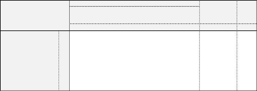
Handbook on Supply and Use Tables and Input-Output Tables with Extensions and Applications
619
20.64 The objective of the price model is to calculate the unknown product prices (price indices)
for exogenously given primary input coefficients which are weighted with the factor price.
20.65 The results for the reference country Germany for the year 2009 are presented in Table
20.8. In this example, it is assumed that the factor price for all primary inputs in all industries is
1.0.
20.66 It should be borne in mind that, for the monetary IOTs of Germany, no information on
quantities and prices (see right-hand side of Box 20.2 and Box 20.3) is available. In consequence,
the input coefficients for primary input must be weighted with a unit price index. The price model
may be used to study the impact of changes in primary inputs (input coefficients, factor prices) on
product prices. When the price model is applied, it is assumed that all conditions of perfect
competition are fulfilled. Higher prices for primary inputs will cause higher product prices in
competitive markets. This approach is capable of simulating the impact of cost-driven inflation;
thus, for example, the price model could be used to study the impact of an increase of the tax on
gasoline on other product prices.
Table 20.8 Price input-output model based on monetary data
Agricul-
ture
Manufac-
turing
Construc-
tion
Trade,
trans.and
comm.
Finance and
business
service
Other
services
Products
(1) (2) (3) (4) (5) (6) (7) (8)
w
Price
index
Agriculture (1)
1.0786 0.2801 0.0383 0.1650 0.2834 0.0225 0.5026 1.0000
Manufacturing (2)
0.0211 1.4040 0.0207 0.1838 0.2155 0.0252 0.5084 1.0000
Construction (3)
0.0050 0.3273 1.0935 0.1548 0.2615 0.0273 0.5042 1.0000
Trade, transport and comm. (4)
0.0024 0.1207 0.0214 1.2805 0.2578 0.0246 0.5786 1.0000
Finance and business
services
(5)
0.0008 0.0411 0.0429 0.0757 1.3775 0.0267 0.6484 1.0000
Other services (6)
0.0021 0.0776 0.0217 0.0920 0.1339 1.0756 0.7517 1.0000
Price
index
Transposed Leontief inverse (I-A')
-1
Products
Input coefficient
for primary inputs

Handbook on Supply and Use Tables and Input-Output Tables with Extensions and Applications
620
Box 20.2 Quantity input-output model
This box shows how the input-output model may be applied to quantities and values.
Agricul-
ture
Manuf. and
const.
Services
Final use Output
Agricul-
ture
Manuf. and
const.
Services
Final use Output
Table 1: Input-output table (quantities)
Table 1: Input-output table (quantities)
Agriculture
4.0
6.8 2.0 8.4
21.2 Agriculture
4.0 6.8 2.0
8.4 21.2
Manuf. and
const.
10.0
76.0 20.0 114.0 220.0
Manuf. and
const.
10.0
76.0
20.0
114.0 220.0
Services
4.0
18.0 8.0 110.5 140.5 Services
4.0 18.0
8.0
110.5 140.5
Labour
5.0 14.0 24.0 43.0 Labour 5.0 14.0 24.0 43.0
Table 2: Prices
Table 2: Prices
Agriculture
Agriculture 5.00 5.00 5.00 5.00
Manuf. and
const.
Manuf. and
const.
2.00
2.00 2.00 2.00
Services
Services 4.00 4.00 4.00 4.00
Labour
10.00
13.00 20.00 Labour 10.00 13.00 20.00
Table 3: Input-output table (values)
Table 3: Input-output table (values)
Agriculture
Agriculture 20.00 34.00 10.00 42.00 106.00
Manuf. and
const.
Manuf. and
const.
20.00
152.00 40.00
228.00 440.00
Services
Services 16.00 72.00
32.00 442.00 562.00
Labour
50.00 182.00 480.00 Labour 50.00 182.00 480.00
712.00
Input
Input 106.00
440.00 562.00 712.00
Table 4: Input coefficients (quantities/quantities) Table 4: Input coefficients (values/values)
Agriculture
0.1887 0.0309 0.0142
Agriculture 0.1887 0.0773 0.0178 0.0590
Manuf. and
const.
0.4717
0.3455 0.1423
Manuf. and
const.
0.1887
0.3455 0.0712
0.3202
Services
0.1887
0.0818 0.0569 Services 0.1509 0.1636
0.0569
0.6208
Labour
0.2358 0.0636
0.1708 Labour 0.4717 0.4136 0.8541
Table 5: Leontief matrix
Table 5: Leontief matrix
Agriculture
0.8113 -0.0309 -0.0142 Agriculture 0.8113 -0.0773
-0.0178
Manuf. and
const.
-0.4717
0.6545 -0.1423
Manuf. and
const.
-0.1887
0.6545
-0.0712
Services
-0.1887 -0.0818 0.9431 Services -0.1509 -0.1636 0.9431
Assumption: Final demand of product B increases by 10%
Assumption: Final demand of product B increases by 10%
Table 6: Leontief inverse Table 6: Leontief inverse
Agriculture
1.2764 0.0639 0.0289 Agriculture 1.2764 0.1597 0.0361
Manuf. and
const.
0.9942
1.6069
0.2576
Manuf. and
const.
0.3977
1.6069
0.1288
Services
0.3416 0.1522 1.0885 Services 0.2733 0.3044 1.0885
Table 7: Quantity input-output model
Table 7: Quantity input-output model
Final use
Output
Final use Output
Agriculture
1.2764 0.0639
0.0289 8.4
21.9 Agriculture 1.2764
0.1597 0.0361 42.00 109.64
Manuf. and
const.
0.9942
1.6069 0.2576 125.4 238.3
Manuf. and
const.
0.3977
1.6069 0.1288 250.80 476.64
Services
0.3416 0.1522
1.0885 110.5 142.2 Services 0.2733 0.3044
1.0885 442.00 568.94
Table 8: Projected input-output table (quantities)
Table 8: Projected input-output table (values)
Agricul-
ture
Manuf. and
const.
Services
Final use TO
Agricul-
ture
Manuf. and
const.
Services
Final use Output
Agriculture
4.1 7.4 2.0 8.4 21.9 Agriculture 20.69 36.83
10.12 42.00 109.64
Manuf. and
const.
10.3
82.3 20.2 125.4 238.3
Manuf. and
const.
20.69
164.66 40.49 250.80 476.64
Services
4.1 19.5 8.1 110.5
142.2 Services 16.55 78.00 32.40 442.00 568.94
Labour
5.2 15.2
24.3 44.6 Labour 51.72 197.15 485.93 734.80
Input
Input 109.64 476.64 568.94 734.80
Table 9: Growth rates in % Table 9: Growth rates in %
Agriculture
3.4 8.3 1.2 3.4 Agriculture 3.4 8.3 1.2 3.4
Manuf. and
const.
3.4
8.3 1.2 10.0 8.3
Manuf. and
const.
3.4
8.3 1.2 10.0 8.3
Services
3.4 8.3 1.2 1.2 Services 3.4 8.3 1.2
1.2
Labour
3.4 8.3
1.2 3.8 Labour 3.4 8.3 1.2 3.2
Input
Input 3.4 8.3 1.2 3.2
Leontief inverse
Leontief inverse
PHYSICAL INPUT-OUTPUT TABLES
MONETARY INPUT-OUTPUT TABLES
Quantities and unit wage rates for labour are known.
Quantities, prices and values are known.

Handbook on Supply and Use Tables and Input-Output Tables with Extensions and Applications
621
Box 20.3 Price input-output model
Agricul-
ture
Manuf. and
const.
Services Final use Output
Agricul-
ture
Manuf. and
const.
Services
Final use Output
Table 1: Input-output table (quantities) Table 1: Input-output table (quantities)
Agriculture
4.0 6.8
2.0 8.4 21.2 Agriculture 4.0 6.8 2.0 8.4 21.2
Manuf. and
const.
10.0
76.0
20.0 114.0 220.0
Manuf. and
const.
10.0 76.0 20.0
114.0
220.0
Services
4.0 18.0
8.0 110.5 140.5 Services 4.0 18.0 8.0 110.5 140.5
Labour 5.0
14.0 24.0 43.0
Labour 5.0 14.0 24.0 43.0
Table 2: Prices Table 2: Prices
Agriculture
Agriculture 5.00 5.00
5.00 5.00
Manuf. and
const.
Manuf. and
const.
2.00 2.00 2.00
2.00
Services Services 4.00 4.00
4.00 4.00
Labour 10.00
13.00
20.00 Labour 10.00 13.00 20.00
Table 3: Input-output table (values)
Table 3: Input-output table (values)
Agriculture Agriculture
20.00
34.00 10.00
42.00 106.00
Manuf. and
const.
Manuf. and
const.
20.00 152.00 40.00 228.00 440.00
Services Services 16.00
72.00 32.00
442.00 562.00
Labour
50.00 182.00 480.00 Labour 50.00 182.00 480.00 712.00
Input
Input 106.00 440.00 562.00 712.00
Table 4: Input coefficients (quantities/quantities) Table 4: Input coefficients (values/values)
Agriculture
0.1887 0.0309 0.0142
Agriculture 0.1887 0.0773 0.0178
Manuf. and
const.
0.4717 0.3455 0.1423
Manuf. and
const.
0.1887 0.3455
0.0712
Services 0.1887 0.0818 0.0569
Services 0.1509 0.1636 0.0569
Labour 0.2358 0.0636 0.1708 Labour 0.4717 0.4136 0.8541
Table 5: Transposed input coefficients intermediates
Table 5: Transposed input coefficients intermediates
Agriculture 0.1887
0.4717 0.1887 Agriculture
0.1887 0.1887 0.1509
Manuf. and
const.
0.0309 0.3455 0.0818
Manuf. and
const.
0.0773 0.3455
0.1636
Services 0.0142 0.1423 0.0569 Services 0.0178 0.0712 0.0569
Table 6: Transposed Leontief matrix
Table 6: Transposed Leontief matrix
Agriculture
0.8113 -0.4717 -0.1887 Agriculture 0.8113 -0.1887 -0.1509
Manuf. and
const.
-0.0309 0.6545 -0.0818
Manuf. and
const.
-0.0773 0.6545 -0.1636
Services -0.0142 -0.1423 0.9431 Services -0.0178 -0.0712 0.9431
Assumption: Price of labour in industry increases by 10% Assumption: Price of labour in industry increases by 10%
Table 7: Price input-output model Table 7: Price input-output model
Primary
inputs
v diag(q)
Product
prices
Primary
inputs
w
Product
price
indexes
Agriculture 1.2764 0.9942 0.3416
2.3585 5.08 Agriculture 1.2764 0.3977 0.2733 0.4717 1.0164
Manuf. and
const.
0.0639 1.6069 0.1522 0.9100 2.13
Manuf. and
const.
0.1597 1.6069 0.3044
0.4550 1.0665
Services 0.0289 0.2576
1.0885 3.4164 4.02 Services 0.0361 0.1288 1.0885 0.8541 1.0053
Table 8: Projected input-output table (values) Table 8: Projected input-output table (values)
Agricul-
ture
Manuf. and
const.
Services Final use Output
Agricul-
ture
Manuf. and
const.
Services Final use Output
Agriculture 20.33 34.56 10.16
42.69 107.74 Agriculture 20.33 34.56 10.16 42.69 107.74
Manuf. and
const.
21.33 162.10
42.66 243.15 469.25
Manuf. and
const.
21.33 162.10
42.66 243.15 469.25
Services 16.09 72.38 32.17 444.35 564.99 Services 16.09 72.38 32.17 444.35 564.99
Labour 50.00
200.20 480.00 730.20 Labour 50.00 200.20 480.00 730.20
Input 107.74 469.25 564.99 730.20 Input 107.74 469.25 564.99 730.20
Table 9: Growth rates in % Table 9: Growth rates in %
Agriculture 1.6 1.6 1.6 1.6 1.6 Agriculture 1.6 1.6 1.6 1.6 1.6
Manuf. and
const.
6.6
6.6 6.6
6.6
6.6
Manuf. and
const.
6.6 6.6 6.6 6.6 6.6
Services 0.5 0.5 0.5 0.5 0.5 Services 0.5 0.5 0.5 0.5 0.5
Labour 0.0 10.0 0.0 2.6 Labour 0.0 10.0 0.0 2.6
Input 1.6 6.6 0.5 2.6 Input 1.6 6.6 0.5 2.6
Transposed inverse
Transposed inverse
PHYSICAL INPUT-OUTPUT TABLES
MONETARY INPUT-OUTPUT TABLES
Quantities and unit wage rates for labour are known.
Quantities, prices and values are known.
Handbook on Supply and Use Tables and Input-Output Tables with Extensions and Applications
622
H. Input-output models with input and output coefficients
20.67 The input-output models that are mainly used in empirical research are based on input
coefficients and are generally called Leontief input-output models. There is, however, another
family of input-output models which are based on output coefficients. These models were
developed by Ambica K. Ghosh (Ghosh, 1958) and are often called Ghosh input-output models.
20.68 The use-side Leontief models reflect x = Ax + f, where x is the output vector, A the Leontief
matrix of technical coefficients and f the supply demand vector. The supply-side Ghosh models
reflect x'B + v' = x', where B is the Ghosh allocation coefficients matrix and v is the added value
vector, the prime indicating the transposition operation. Both models may be used to study the
impact of changes in final use and primary inputs on output, and also price and cost effects. The
dual character of Leontief models and Ghosh models is discussed in Oosterhaven (1996),
Dietzenbacher (1997), de Mesnard (2009) and Rueda-Cantuche (2011). Input-output models may
also be used to estimate the forward and backward linkages of industries. The input coefficients
reflect production functions and cost structures of activities, whereas the output coefficients reflect
distribution parameters for products and primary inputs reflecting market shares and sales
structure.
20.69 The use of input coefficients and output coefficients in input-output analysis is
demonstrated for the four basic input-output models with input and output coefficients. The four
input-output models have a dual character with an underlying symmetry. Each input-output model
with input coefficients has a complement with output coefficients. Leontief and Ghosh models are
similar but opposite in structure, almost mirror images of one another. Leontief models use fixed
input coefficients, while Ghosh models rely on fixed output coefficients. The four models may be
summarized as follows:
• The Leontief quantity model is a use-driven model which is often used to study the impact
of an exogenous change of final uses on output. It is based on the accounting identities for
total output along the rows of IOTs and uses fixed intermediate and primary input
coefficients.
• The Leontief price model is sometimes also called the “cost-push input-output price model”
and allows the simulation of cost-driven inflationary processes by simulating the impact of
price changes of primary inputs on product prices (inflation). The primary input prices are
assumed to be exogenous, whereas the prices for outputs are determined by the solution of
the model.
• The traditional Ghosh quantity model was formulated as a supply-driven model and was
developed to study the impact of an increase in primary inputs on output and final use. The
Ghosh quantity model starts with the accounting identities for total input along the columns
of an IOT. Instead of exogenous final use, the Ghosh quantity model has exogenous primary
inputs and produces a solution for endogenous total inputs. Final use forms a residual and is
Handbook on Supply and Use Tables and Input-Output Tables with Extensions and Applications
623
taken as granted. The input ratios for intermediate consumption vary arbitrarily and essential
production requirements are ignored.
• The traditional Ghosh price model was designed as a demand-driven price model. The single
price for each column of final use is exogenous and the prices for intermediate consumption
and primary inputs are endogenous variables. The model describes the cumulative effects of
changes in final output prices on unit revenues per industry and prices of primary inputs such
as labour and the use of capital. If the price of a specific product of final use is increasing,
then the price for all inputs of an industry would increase at the same rate causing an unusual
impact on inflation.
20.70 The outcome of the traditional Ghosh models, by comparison with Leontief models, is
difficult to interpret in economic terms, and this has given rise to many disagreements. In response
to the criticism levelled against Ghosh models and to remedy their implausibility, Dietzenbacher
(1997) proposed an alternative interpretation by suggesting that the model be viewed, not as a
quantity model, but as a price model, following Miller and Blair (2009, p. 551). De Mesnard (2009,
pp. 364 and 370) also showed that the so-called equation of the Ghosh model (x'B + v' = x') is
actually that of the Ghosh model in physical terms, hence it cannot be compared to the equation
of the Leontief model (x = Ax + f).
20.71 It remains to be seen in empirical research whether the input coefficients or output
coefficients are more stable over time and behave according to expectations. It is easy to
understand, however, why input-output models with output coefficients are rarely used in
empirical research, since they lack a proper microeconomic foundation. Input-output models with
input coefficients are well established in economic analysis. At best, such models reflect the cost
structure of industries and the input structure of final use components. At the same time, it is the
rigidity of the underlying Leontief production functions which poses an obstacle to many
applications.
I. Central model of input-output analysis
20.72 Input-output analysis has often been used to study the impact of final use on output
(quantity model) and value added changes on prices (price model). Appropriate extensions of the
input-output system also allow evaluation of the direct and indirect impact of economic policies
on other economic variables, such as labour, capital, energy and emissions (joint product). Most
of these policy issues, such as labour policy, structural policy and fiscal policy, must be analysed
with macroeconomic models which provide a minimum of industrial and product disaggregation.
20.73 The following extension of the input-output equation system offers multiple approaches
for analysis:
Central equation of input-output analysis:
(41) =
(
)
Handbook on Supply and Use Tables and Input-Output Tables with Extensions and Applications
624
= matrix of input coefficients for specific variable in economic analysis (intermediate
consumption, labour, capital, energy, etc.)
= unit matrix
= matrix of input coefficients for intermediate consumption
= diagonal matrix for final use
= matrix with results for direct and indirect requirements (intermediates, labour, capital,
energy, emissions, etc.)
20.74 Matrix includes the input coefficients of the variable under investigation (intermediates,
labour, capital, energy, emissions, and others). The diagonal matrix denotes exogenous final use
for goods and services. The matrix incorporates the results for the direct and indirect
requirements (intermediates, labour, capital, energy) or joint outputs (emissions) for the produced
goods and services of final use.
20.75 In essence, this approach makes it possible to assess the total (direct and indirect) primary
energy requirements or carbon dioxide emissions in the production of a vehicle occurring at all
stages of production, up to the provision of the product (vehicle) to a final user. It should be noted
that this approach focuses on domestic emissions only and not the total emissions. The part
constituted by emissions related to imported products is missing and these can be taken on board
by using total IOTs instead of the domestic part only and applying domestic technology
assumptions.
20.76 Corresponding calculations of the labour and capital content of products are also feasible
with this equation. Direct contributions of final users (for example, direct emissions of carbon
dioxide by private households) must be added as column vectors to the results of matrix to
account for the total emissions of final use.
20.77 This type of analysis is based on the restrictive assumptions of input-output models.
Although these assumptions could be viewed as weakly based, this input-output analysis at least
offers opportunities to assess the magnitude of the expected effects in the short term, through the
allocation of responsibility for emissions to final use by linking final use products and emissions
of industries. In Table 20.9, a corresponding calculation is presented for the emission of three
disposals to nature, namely the gases carbon dioxide (CO
2
), methane (CH
4
) and nitrous oxide
(N
2
O). The variable at the bottom of Table 20.9 also reflects the direct emissions of private
households.

Handbook on Supply and Use Tables and Input-Output Tables with Extensions and Applications
625
Table 20.9 Emission model
Germany 2009
20.78 In Table 20.9, the actual direct emissions (rows (1)–(3)) and total output levels of
production (row (4)) are reported. In rows (5)–(7) the corresponding emission coefficients have
been calculated. The lowest carbon dioxide emission coefficient, 11.957 (1,000 tons of emissions
per 1 billion euros), is reported for “Business services” in column (5). The results in row (14)
reveal, however, that the inclusion of indirect emissions results in a higher value of emission
coefficient, 41.586, for “Business services”. The estimates in column (5) and row (14) include all
direct and indirect emissions of carbon dioxide which can be related to the production of one unit
of output of “Business services” at all stages of production.
20.79 As shown in row (17) of Table 20.9, the industry “Agriculture” is delivering goods and
services in the magnitude of 18.003 billion euros for final use. The calculation reveals that, in the
Households Government
(1) (2)
(3) (4)
(5)
(6) (7)
(8) (9) (10) (11) (12)
Carbon dioxide (CO
2
)
(1) 9 260
550 893 9 162
80 990 12 077
24 173
222 268
908 823
Methane (CH
4
)
(2) 1 247
925 1
49 3 10 79 2 313
Nitrous oxide (N
2
O)
(3)
137 62 2 4
206
Output at basic prices (4) 42 1 451 234 907 1 010 721
Carbon dioxide (CO
2
)
(5)
219.813 379.615 39.115 89.336 11.957 33.541
Methane (CH
4
)
(6)
29.609 0.637 0.004 0.054 0.003 0.014
Nitrous oxide (N
2
O)
(7) 3.257 0.043
0.001 0.002
0.000 0.000
Agriculture (8) 1.0786 0.0211
0.0050 0.0024
0.0008 0.0021
Manufacturing (9)
0.2801 1.4040 0.3273
0.1207 0.0411 0.0776
Construction (10) 0.0383 0.0207 1.0935 0.0214 0.0429 0.0217
Trade, transport and comm. (11) 0.1650 0.1838 0.1548 1.2805 0.0757 0.0920
Finance and business services (12) 0.2834 0.2155 0.2615 0.2578 1.3775 0.1339
Other services (13) 0.0225 0.0252 0.0273 0.0246 0.0267 1.0756
Carbon dioxide (CO
2
)
(14) 363.803 558.261 186.001 165.476
41.586 76.668
Methane (CH
4
)
(15) 32.126 1.530 0.371 0.219 0.059 0.132
Nitrous oxide (N
2
O)
(16) 3.526 0.129 0.031 0.016 0.005 0.011
Agriculture (17) 18.003 0.000 0.000 0.000
0.000 0.000
Manufacturing
(18) 0.000 904.835 0.000 0.000 0.000 0.000
Construction (19) 0.000 0.000 158.546 0.000 0.000 0.000
Trade, transport and comm. (20) 0.000 0.000 0.000 487.822 0.000 0.000
Finance and business services (21) 0.000 0.000 0.000 0.000 405.957 0.000
Other services (22) 0.000 0.000 0.000 0.000 0.000 623.171
Carbon dioxide (CO
2
)
(23) 6 550 505 134 29 490 80 723 16 882 47 777 222 268 908 823
Methane (CH
4
)
(24) 578 1 384 59 107 24 82
79
2 313
Nitrous oxide (N
2
O)
(25) 63 117 5 8 2 7 4 206
Total
output at
basic
prices
Products
Final use
Direct emissions (1000 tons)
Final consumption
Gross
fixed
capital
Changes
in
inventories
Exports
Agricul-
ture
Manufac-
turing
Construc-
tion
Trade,
trans.and
comm.
Finance
and
business
Other
services
Direct and indirect emissions per unit of output B(I-A)
-1
Diagonal matrix of final demand Y
Emission content of final demand (1000 tons) Z = B(I-A)
-1
Y + Eh
Output (Billions euros)
Emission coefficients (1000 tons per billions euros)
Inverse (I-A)
-1
Handbook on Supply and Use Tables and Input-Output Tables with Extensions and Applications
626
course of production, 6.550 million tons of carbon dioxide have been emitted in Germany across
all stages of production, up to the provision of these agricultural products to final use.
20.80 The industry “Manufacturing” has the largest emissions at this level of aggregation and it
includes mining and electricity. This industry is directly responsible for the emission of 550.893
million tons of carbon dioxide in own plants, as shown in row (1) of Table 20.9. In terms of the
number of tons of carbon dioxide emitted on all stages of production to produce manufactured
goods for final use (904.825 billion euros), 505.134 million tons of carbon dioxide emissions may
be attributed to products of manufacturing for final use. A corresponding interpretation of the
results is valid for all industries of the economy. This approach makes possible the reallocation of
the emissions of carbon dioxide to the products purchased by final use. Again, it should be noted
that this approach applies only to emissions on domestic territory and not to emissions released
during production of imported products used in the production processes.
20.81 The total emissions of carbon dioxide are reported in column (12) of Table 20.9 with
908.823 million tons for the economy. Column (7) of Table 20.9 shows that household
consumption is responsible for the direct emission of 222.268 million tons of carbon dioxide. The
results in the last part of Table 20.9 include estimates for emissions attributed to final use
categories. The direct emissions of household consumption must be added as a separate column
vector to the matrix to attain the national emission total of 908.823 million tons of carbon
dioxide, as shown in row (23) in Table 20.9.
20.82 This example demonstrates how extended input-output based systems may be used
effectively to evaluate environmental policies. This tool will enable analyses of whether national
emissions reduction targets are met and how they comply with the Kyoto Agreement and the
targets of the Intergovernmental Panel on Climate Change. At the same time, the same database
can be used for other important fields of economic analysis, such as the impact of employment
policies, substitution of labour and capital, productivity analysis, energy issues, environmental
problems or structural policies.
J. Indicators
20.83 In general, in the neo-classical microeconomic approach, it is assumed that the production
function relates the amount of inputs used by an industry to the maximum amount that can be
produced by that industry with its primary inputs.
Production function:
(42)
=
,
,
= output of industry (products)
= inter-industry flow (goods, services) from sector to sector (intermediate consumption)
= labour requirements of sector
Handbook on Supply and Use Tables and Input-Output Tables with Extensions and Applications
627
= capital requirements of sector
= technology
20.84 In input-output analysis, a fundamental assumption is that for a given period the inter-
industry flows of products (
) from industry to industry and primary inputs (, ) depend on
the total output of industry (
). If constant returns to scale and fixed relations of all inputs are
assumed, then a set of technical input coefficients that reflect the technology can be produced. In
most production processes, different products are produced but different labour skills and different
types of capital goods are also required. Accordingly, the set of input coefficients in a broader
notation of the matrix encompasses input coefficients for products (intermediate consumption),
capital and labour (primary inputs).
Technical input coefficients:
(43)
=
/
= input coefficient
= input of type in sector (products, capital, labour)
= output of sector (product)
20.85 Using the definitions of the technical input coefficients, the production can be specified in
the following form:
Leontief production function:
(44)
= min
/
,
/
, … ,
/
20.86 A number of input variables for various branches have been summarized in Table 20.10.
These represent input requirements for products (intermediate consumption), labour, capital and
energy. The following set of coefficients for emissions has a different character. In each production
activity and each consumption activity, certain pollutants are emitted as joint products (disposals
to nature). The corresponding emission coefficients for carbon dioxide and nitrous oxide are
summarized using international standard weights to identify the impact on global warming and
acid deposition.

Handbook on Supply and Use Tables and Input-Output Tables with Extensions and Applications
628
Table 20.10 Input indicators for production activities per unit of output
Germany 2009
Agricul-
ture
Manufac-
turing
Construc-
tion
Trade,
trans.and
comm.
Finance and
business
service
Other
services
(1) (2) (3) (4) (5) (6)
Domestic goods and services (1) 0.497 0.492 0.496 0.421 0.352 0.248
Imported goods and services (2) 0.109 0.195 0.074 0.064 0.030 0.029
Intermediate consumption (3) 0.607 0.687 0.569 0.485 0.382 0.277
Taxes less subsidies on products (4) 0.036 0.007 0.008 0.013 0.016 0.034
Compensation of employees (5) 0.134 0.212 0.294 0.325 0.189 0.505
Other net taxes on production (6) -0.141 -0.002 -0.001 -0.001 0.004 -0.010
Consumption of fixed capital (7) 0.189 0.054 0.022 0.066 0.158 0.088
Operating surplus, net (8) 0.174 0.041 0.108 0.111 0.250 0.106
Value added at basic prices (9) 0.357 0.306 0.423 0.501 0.602 0.689
Machinery (10) 0.052 0.014 0.007 0.021 0.081 0.040
Buildings (11) 0.125 0.033 0.017 0.050 0.115 0.051
Total (12) 0.177 0.047 0.023 0.070 0.196 0.090
Machinery (13) 3.963 0.716 0.348 0.857 6.929 3.112
Buildings (14) 2.466 0.445 0.216 0.533 0.527 0.335
Total (15) 6.430 1.161 0.564 1.391 7.456 3.446
Wage and salary earners (16) 7,002 4,677 8,317 10,833 5,637 15,757
Self-employed (17) 8,522 189 1,977 1,431 1,007 1,469
Total (18) 15,524 4,866 10,293 12,264 6,643 17,227
Coal and coal products (19) 0.009 1.181 0.002 0.001 0.000 0.008
Brown coals and lignite products (20) 0.002 1.114 0.001 0.000 0.000 0.001
Crude oil (21) 2.959
Gasolines (22) 0.083 0.063 0.019 0.028 0.020 0.021
Diesel fuels (23) 2.525 0.084 0.338 0.525 0.092 0.103
Jet fuels (24) 0.478 0.005
Heating oil, light (25) 0.582 0.130 0.060 0.096 0.026 0.118
Fuel oil, heavy (26) 0.231 0.019 0.000 0.000
Other petroleum products (27) 0.043 0.820 0.433 0.039 0.002 0.004
Natural gas and other gases (28) 0.291 1.238 0.050 0.138 0.049 0.256
Renewable Energy (29) 0.142 0.812 0.019 0.050 0.007 0.008
Electric power and other energy (30) 0.542 1.820 0.058 0.319 0.075 0.273
Total (31) 4.220 10.452 0.980 1.694 0.270 0.797
Carbon dioxide (CO
2
) (32) 219.813 379.615 39.115 89.336 11.957 33.541
Methane (CH
4
) (33) 29.609 0.637 0.004 0.054 0.003 0.014
Nitrous oxide (N
2
O) (34) 3.257 0.043 0.001 0.002 0.000 0.000
Nitrogen oxides (NOx) (35) 3.624 0.371 0.195 0.440 0.033 0.062
Sulfur dioxide (SO
2
) (36) 0.064 0.257 0.005 0.045 0.002 0.011
Organic compounds (NMVOC) (37) 0.313 0.395 0.024 0.044 0.003 0.010
Ammonia (NH
3
) (38) 12.835 0.011 0.001 0.003 0.000 0.001
Particulate matter (PM
10
) (39) 1.125 0.029 0.029 0.047 0.002 0.004
Hydroflurocarbons (HFC) (40) 0.008 0.001
Perflurorocarbons (PFC) (41) 0.000
Sulfur hexafluoride (SF
6
) (42) 0.000
Total (43) 270.640 381.366 39.373 89.969 11.999 33.642
Greenhouse gases (44) 1851.272 406.193 39.412 91.233 12.074 33.971
Acid deposition (45) 2.600 0.516 0.141 0.352 0.025 0.054
Tropospheric ozone formation (46) 33.545 1.403 0.223 0.537 0.038 0.085
Waste (1000 tons) (47) 19.073 84.654 828.662 5.455 5.455 5.455
Sewage (million cu m) (48) 0.504 18.585 0.161 0.191 0.191 0.191
Water from waterworks (million cu m) (49) 3.228 -2.567 0.058 0.214 0.214 0.214
Water from nature (million cu m) (50) 7.200 25.915 0.105 0.010 0.010 0.010
Prooducts
Intermediate consumption (billion euros)
Taxes less subsidies on products (billion euros)
Waste, sewage and water
Value added (billion euros)
Gross fixed capital formation (billion euros)
Capital stock (billion euros)
Employment (Persons)
Energy (Petajoule)
Em issi ons (1000 ton s)
Global warming and acid deposition (1000 tons)
Handbook on Supply and Use Tables and Input-Output Tables with Extensions and Applications
629
K. Multipliers
20.87 Three of the most frequently used types of multipliers in input-output analysis are those
that estimate the effects of the exogenous changes of final use on:
• Outputs of the industries (and products) in the economy
• GVA and income earned by the households
• Employment, that is expected to be generated by the new activity levels
20.88 In the standard input-output model, the final use categories are considered exogenous
variables. In many respects, however, household final consumption expenditure and gross fixed
capital formation depend on the income of private households (and businesses). In the type I
multiplier analysis, household final consumption expenditure and, consequently, private
household activities are exogenous. A more refined type II multiplier analysis for wages and
private consumption is designed to include the household sector as an endogenous activity. It is
assumed that, to a large extent, the income earned by private households from wages and salaries
is spent as household final consumption expenditure. This additional income induces higher
incomes, which again induce more household final consumption expenditure until a new
equilibrium is reached.
20.89 Box 20.4 provides analysis of the type I and type II multiplier links for the output
multiplier, income multiplier and employment multiplier to the input-output model.
1. Output multipliers
20.90 An output multiplier for an industry is defined as the total value of production in all
industries of the economy that is necessary for all stages of production in order to produce one unit
of product for final use. The output multiplier in Table 20.11 corresponds to the column sum of
the Leontief inverse as shown in Table 20.6.
Table 20.11 Output multipliers (Leontief inverse)
Agricul-
ture
Manufac-
turing
Construc-
tion
Trade,
trans.and
comm.
Finance and
business
service
Other
services
(1) (2)
(3) (4) (5) (6)
Agriculture (1)
1.0786 0.0211 0.0050 0.0024 0.0008 0.0021
Manufacturing (2) 0.2801 1.4040 0.3273 0.1207 0.0411 0.0776
Construction (3) 0.0383 0.0207 1.0935 0.0214 0.0429 0.0217
Trade, transport and comm. (4) 0.1650 0.1838 0.1548 1.2805 0.0757 0.0920
Finance and business services (5) 0.2834 0.2155 0.2615 0.2578 1.3775 0.1339
Other services (6) 0.0225 0.0252 0.0273 0.0246 0.0267 1.0756
Total (7) 1.8679 1.8704 1.8695 1.7074 1.5648 1.4029
Handbook on Supply and Use Tables and Input-Output Tables with Extensions and Applications
630
20.91 If a government agency, for example, wished to determine in which industry of the
economy to spend additional money, a comparison of output multipliers would indicate where this
spending would have the greatest impact in terms of the total value of output generated throughout
the economy. In this case, it would be the industry “Manufacturing”, with an output multiplier of
= 1.8704. If the elements of the inverse ( )
are represented as
, then the output
multiplier may be defined as:
Output multiplier:
(45)
=
20.92 The output multiplier in row (7) of Table 20.11 represents for each industry one unit of
final use (1.0) and the direct and indirect requirements for domestic intermediate consumption, for
example, for agriculture, 0.8679. Multipliers of this sort may overstate or understate the effect on
the economy, for example, if some industries are operating at capacity and a process of substitution
with imported inputs could take place. Another critical element is the internal consumption of an
industry on the diagonal of its own products.
20.93 Depending upon the statistical sources, the aggregation of survey results may have a
distinct influence on the magnitude of the reported internal consumption.
2. Income multipliers
20.94 Income multipliers attempt to identify the impacts of final use changes on income received
by households (labour supply). The central equation (41) of the input-output models is used to
calculate the direct and indirect requirements for wages which are incorporated in one unit of
output for final use. This calculation is equivalent to an assessment of the wage content of products.
Direct and indirect requirements for wages:
(46) = ()
= vector of input coefficients for wages
= unit matrix
= matrix of input coefficients for intermediate consumption
= vector with results for direct and indirect requirements for wages

Handbook on Supply and Use Tables and Input-Output Tables with Extensions and Applications
631
Box 20.4 Multipliers in the input-output model
The type I and type II multiplier links for the output multiplier, income multiplier and employment multiplier to the input-
output model are shown below.
20.95 In Table 20.12, various multipliers are summarized for products which are delivered to
final use. In our numerical example, the industry “Agriculture” has a relatively small direct input
coefficient for wages, as exemplified by
= 0.134 in Table 20.10, reflecting that a significant
proportion of the working population in agriculture is self-employed.
Input-output table Billion euros
Households Government
Products
(1) (2) (3) (4) (5) (6) (7) (8) (9) (10) (11) (12)
Agriculture (1) 3 20 1 9 3 5 42
Manufacturing (2) 7 394 48 56 11 30 250 7 95 - 58 611 1 451
Construction (3) 1 11 18 8 28 10 5 153 1 234
Trade, transport and
comm.
(4) 4 139 17 181 38 40 317 15 39 6 111 907
Finance and business
services
(5) 6 131 30 124 261 51 313 3 25 66 1 010
Other services (6) 18 3 12 17 47 147 472 2 2 721
Total at basic prices (7) 21 713 116 382 355 179 1 041 497 314 - 49 795 4 365
Imports (8) 5 283 17 58 31 21 128 9 61 31 189 833
Taxes less subsidies on
products
(9) 2 10 2 12 17 24 151 6 34 257
Total at purchasers’ prices (10) 27 1 007 135 452 402 224 1 319 513 409 - 18 984 5 455
Compensation of
employees
(11) 6 308 69 294 191 364 1 232
Other taxes less subsidies
on production
(12) - 6 - 2 - 1 5 - 7 - 12
Consumption of fixed
capital
(13) 8 79 5 60 160 63 375
Net operating surplus (14) 7 60 25 101 252 77 523
GVA (15) 15 445 99 454 608 497 2 117
Input (16) 42 1 451 234 907 1 010 721 1 319 513 409 - 18 984
Employment 1000 Persons
Employment (17) 654 7 062 2 411 11 118 6 710 12 415 40 370
Germany 2009 Empty cells
Type I multiplier analysis Type II multiplier analysis
with exogenous final demand with endogenous households consumption and labour income
Input coeffici ents (A) Input coefficients (A)
0.0692 0.0139 0.0000 0.0004 0.0001 0.0008 0.0692 0.0139 0.0000 0.0004 0.0001 0.0008 0.0071
0.1686 0.2716 0.2048 0.0619 0.0110 0.0414 0.1686 0.2716 0.2048 0.0619 0.0110 0.0414 0.1894
0.0219 0.0077 0.0749 0.0088 0.0278 0.0139 0.0219 0.0077 0.0749 0.0088 0.0278 0.0139 0.0035
0.0838 0.0956 0.0739 0.2000 0.0377 0.0552 0.0838 0.0956 0.0739 0.2000 0.0377 0.0552 0.2407
0.1443 0.0906 0.1284 0.1370 0.2584 0.0712 0.1443 0.0906 0.1284 0.1370 0.2584 0.0712 0.2370
0.0095 0.0122 0.0138 0.0132 0.0166 0.0659 0.0095 0.0122 0.0138 0.0132 0.0166 0.0659 0.1113
0.1342 0.2122 0.2939 0.3248 0.1893 0.5055 0.0000
Leonti ef i nver se (I -A)
-1
Leonti ef i nver se (I -A)
-1
1.0786 0.0211 0.0050 0.0024 0.0008 0.0021 1.0852 0.0293 0.0149 0.0124 0.0071 0.0142 0.0195
0.2801 1.4040 0.3273 0.1207 0.0411 0.0776 0.4430 1.6090 0.5737 0.3691 0.1974 0.3811 0.4879
0.0383 0.0207 1.0935 0.0214 0.0429 0.0217 0.0516 0.0374 1.1136 0.0416 0.0557 0.0464 0.0398
0.1650 0.1838 0.1548 1.2805 0.0757 0.0920 0.3570 0.4254 0.4453 1.5733 0.2599 0.4496 0.5750
0.2834 0.2155 0.2615 0.2578 1.3775 0.1339 0.5138 0.5053 0.6098 0.6091 1.5984 0.5628 0.6896
0.0225 0.0252 0.0273 0.0246 0.0267 1.0756 0.0931 0.1140 0.1341 0.1322 0.0944 1.2070 0.2113
0.5151 0.6479 0.7788 0.7854 0.4939 0.9591 1.5419
Column sum of input coefficient for intermediates Column sum of input coefficient for intermediates
0.4974 0.4916 0.4958 0.4214 0.3516 0.2483 0.6316 0.7038 0.7896 0.7461 0.5409 0.7538 0.7890
Output multiplier OM = column sum of Leontief inverse Output multiplier OM = column sum of Leontief inverse
1.8679 1.8704 1.8695 1.7074 1.5648 1.4029 3.0587 3.3683 3.6702 3.5232 2.7068 3.6203 3.5649
Input coefficient for compensation of employees w Input coefficient for compensation of employees w
0.1342 0.2122 0.2939 0.3248 0.1893 0.5055 0.1342 0.2122 0.2939 0.3248 0.1893 0.5055 0.0000
Income multiplier IM = w(I-A)
-1
Income multiplier IM = w(I-A)
-1
0.3340 0.4202 0.5051 0.5093 0.3203 0.6220 0.5151 0.6479 0.7788 0.7854 0.4939 0.9591 0.5419
Input coefficient for employment m Input coefficient for employment m
15.524 4.866 10.293 12.264 6.643 17.227 15.524 4.866 10.293 12.264 6.643 17.227 0.000
Employment multiplier EM = m(I-A)
-1
Employment multiplier EM = m(I-A)
-1
22.796 11.494 17.034 18.686 11.194 21.180 28.928 19.208 26.307 28.037 17.076 32.599 18.359
Output multiplier
Products
Final use
Output
Agricul-
ture
Manufac-
turing
Construc-
tion
Trade,
trans.and
comm.
Finance
and
business
Other
services
Final consumption
Gross fixed
capital
formation
Changes
in
inventories
Exports
Employment multiplier
The employment multiplier for sector j is defned as the total number of persons employed in all sectors of the
economy that is necessary to produce one million dollar's worth of final demand of product j.
The output multiplier for sector j is defined as the total value of production in all sectors of the economy that is
necessary to produce one dollar's worth of final demand of product j.
Income multiplier
The income multiplier for sector j is defined as the total value of all wages in all sectors of the economy that is
necessary to produce one dollar's worth of final demand of product j.

Handbook on Supply and Use Tables and Input-Output Tables with Extensions and Applications
632
Table 20.12 Multipliers for products
Germany 2009
Agricul-
ture
Manufac-
turing
Construc-
tion
Trade,
trans.and
comm.
Finance and
business
service
Other
services
(1) (2) (3) (4) (5) (6)
Final demand of domestic products (1) 1.000 1.000 1.000 1.000 1.000 1.000
Intermediate demand of domestic products (2) 0.868 0.870 0.870 0.707 0.565 0.403
Imported products (3) 0.195 0.297 0.164 0.116 0.059 0.058
Taxes less subsidies on products (4) 0.049 0.018 0.018 0.023 0.025 0.041
Products at purchasers' prices (5) 1.112 1.185 1.051 0.847 0.649 0.501
Compensation of employees (6) 0.334 0.420 0.505 0.509 0.320 0.622
Other net taxes on production (7) -0.151 -0.005 -0.001 -0.001 0.006 -0.011
Consumption of fixed capital (8) 0.278 0.129 0.096 0.135 0.228 0.127
Operating surplus, net (9) 0.295 0.141 0.218 0.217 0.362 0.164
Value added at basic prices (10) 0.756 0.686 0.818 0.861 0.916 0.902
Machinery (11) 0.088 0.043 0.038 0.050 0.115 0.057
Buildings (12) 0.186 0.085 0.069 0.099 0.166 0.078
Total (13) 0.274 0.128 0.107 0.149 0.281 0.135
Machinery (14) 6.664 2.825 2.664 3.064 9.740 4.425
Buildings (15) 3.038 0.902 0.624 0.891 0.805 0.524
Total (16) 9.702 3.727 3.288 3.956 10.545 4.949
Wage and salary earners (17) 12.921 10.491 14.242 16.472 9.560 19.257
Self-employed (18) 9.875 1.004 2.791 2.214 1.634 1.922
Total (19) 22.796 11.494 17.034 18.686 11.194 21.180
Coal (20) 0.341 1.658 0.389 0.144 0.049 0.101
Lignite (21) 0.314 1.564 0.365 0.135 0.046 0.087
Crude oil (22) 0.829 4.154 0.968 0.357 0.122 0.230
Natural gas (23) 0.118 0.100 0.052 0.050 0.034 0.033
Nuclear fuels (24) 2.876 0.298 0.518 0.722 0.190 0.191
Water power (25) 0.079 0.088 0.074 0.613 0.036 0.049
Briquettes (26) 0.692 0.222 0.135 0.151 0.054 0.152
Coke (27) 0.068 0.328 0.079 0.052 0.011 0.020
Petroleum products (28) 0.300 1.169 0.749 0.159 0.058 0.081
Electricity (29) 0.705 1.788 0.502 0.347 0.137 0.392
Produced gas (30) 0.392 1.154 0.297 0.165 0.048 0.078
Steam, hot water (31) 1.177 2.650 0.739 0.656 0.213 0.477
Total (32) 7.891 15.173 4.869 3.550 0.997 1.891
Carbon dioxide (CO
2
) (33) 363.803 558.261 186.001 165.476 41.586 76.668
Methane (CH
4
) (34) 32.126 1.530 0.371 0.219 0.059 0.132
Nitrous oxide (N
2
O) (35) 3.526 0.129 0.031 0.016 0.005 0.011
Sulfur dioxide (SO
2
) (36) 4.103 0.690 0.431 0.630 0.107 0.152
Nitrogen oxides (NO
x
) (37) 0.149 0.371 0.097 0.089 0.017 0.036
Carbon monoxide (CO) (38) 0.457 0.571 0.165 0.106 0.025 0.046
Organic compounds (NMVOC) (39) 13.848 0.286 0.070 0.036 0.012 0.029
Dust particles (40) 1.232 0.074 0.055 0.068 0.010 0.014
Total (41) 0.002 0.011 0.003 0.001 0.000 0.001
Greenhouse gases (42) 2,131.379 630.364 203.533 175.135 44.363 82.822
Acid deposition (43) 3.021 0.854 0.399 0.531 0.091 0.143
Tropospheric ozone formation (44) 36.686 2.791 0.966 0.956 0.190 0.331
Waste (1000 tons/billion euros) (45) 78.594 138.761 936.398 36.517 47.149 31.694
Sewage (million cu m/billion euros) (46) 5.845 26.188 6.346 2.545 1.053 1.695
Water from waterworks (million cu m/billion euros) (47) 2.866 -3.444 -0.665 0.034 0.216 0.087
Water from nature (million cu m/billion euros) (48) 15.033 36.542 8.638 3.162 1.089 2.041
Value added (billion euros/billion euros)
Gross fixed capital formation (billion euros/billion euros)
Domestic production (billion euros/billion euros)
Products
Emissions (1000 tons/billion euros)
Global warming and acid deposition (1000 tons/billion euros)
Waste, sewage and water
Capital stock (billion euros/billion euros)
Employment (1000 persons/billion euros)
Energy (Petajoule/billion euros)
Handbook on Supply and Use Tables and Input-Output Tables with Extensions and Applications
633
20.96 If, however, we calculate the income multiplier for wages (direct and indirect wage
requirements per unit of output) for this industry,
= 0.334 as shown in Table 20.12, we can
verify that the “wage content” of agricultural products is tripled. Thus, the intermediate
consumption inputs of agriculture incorporate a significant amount of wages.
20.97 Similarly, the category “Other services” has the highest direct (
= 0.505) and direct
and indirect (
= 0.622) wage requirements. This general approach makes it possible to assess
the wage, labour, capital or energy content of the various components of final use.
3. Employment multipliers
20.98 When employment multipliers are calculated, the major difference in the calculation of the
wage content of products is that the physical labour input coefficients are used instead of monetary
labour input coefficients.
Direct and indirect requirements for labour:
(47) = ()
= matrix of input coefficients for labour (1,000 persons per billion euros of output)
= matrix with results for direct and indirect requirements for labour (persons)
20.99 For each industry, the employment multipliers represent jobs created per unit of currency
of additional final use. The labour-intensive industry “Agriculture” has the highest employment
multiplier,
= 22.796. If the final use for agricultural products were increased by 1 billion
euros, 22,796 positions (wage and salary earners and self-employed) would be created in this
industry. However, the largest difference between direct employment coefficients and employment
multipliers (direct and indirect employment) is observed in “Manufacturing”.
4. Capital multipliers
20.100 The satellite systems shown in table 19.3 include information on labour and capital, which
is required for the production of the various industries. The matrix for labour distinguishes between
wage and salary earners and the self-employed, in separate rows, while the matrix for capital stock
provides data for machinery and buildings. This database makes it possible to assess the labour
and capital content of products and also the direct and indirect substitution of labour and capital,
provided that a time series of IOTs with the corresponding satellite systems is available.
20.101 Monetary input coefficients for capital are used to calculate the capital content of products
using the following equation:
Direct and indirect requirements for capital:
(48) =
(
)
C = matrix of input coefficients for capital requirements per unit of output
Handbook on Supply and Use Tables and Input-Output Tables with Extensions and Applications
634
Z = matrix with results for direct and indirect requirements of capital
20.102 The calculation reveals that the highest capital multiplier (capital intensity) is for “Business
services”. The direct capital requirements in this industry are
= 7.456, as shown in Table
20.10.
20.103 The capital multipliers in Table 20.12 reflect the direct and indirect capital requirements at
all stages of production. To produce 1 million euros of “Business services” for final use, 10.545
billions of Euros capital (buildings, machinery) are required (
= 10.545 ) at all stages of
production.
5. Primary input content of final use
20.104 The multipliers enable assessment of the primary input content of final use by product and
by category. The results are presented in Table 20.13 for the primary input content of final use by
category.
20.105 For the various products of final use, the multipliers for primary inputs
(
)
are
multiplied with a diagonal matrix of final use total for products.
Direct and indirect requirements for primary inputs:
(49) =
(
)
= matrix of input coefficients for primary input
= unit matrix
= matrix of input coefficients for intermediate consumption
= Diagonal matrix for final use by product
= matrix with results for direct and indirect requirements for primary inputs
(50) =
(
)
Direct and indirect requirements for primary inputs
= matrix of input coefficients for primary input
= matrix of final use by category
= matrix with results for direct and indirect requirements for primary inputs

Handbook on Supply and Use Tables and Input-Output Tables with Extensions and Applications
635
Table 20.13 Input content of final use by category
Germany 2009
Households Governmnet
(1) (2) (3) (4) (5) (6)
Total (1) 1 041 497 314 - 49 795 2 598
Domestic products (2) 690 209 258 - 44 653 1 767
Imported products (3) 140 31 59 - 16 199 414
Taxes less subsidies on products (4) 26 20 6 - 1 15 67
Products at purchasers' prices (5) 856 260 323 - 60 868 2 247
Compensation of employees (6) 464 305 146 - 20 337 1 232
Other net taxes on production (7) - 3 - 5 - 1 0 - 3 - 12
Consumption of fixed capital (8) 168 63 38 - 6 111 375
Operating surplus, net (9) 245 83 64 - 6 136 523
Value added at basic prices (10) 874 446 248 - 32 581 2 117
Machinery (11) 72 28 15 - 2 40 153
Buildings (11) 118 39 27 - 4 75 255
Total (12) 190 67 42 - 6 115 409
Machinery (13) 5 449 2 182 1 045 - 126 2 755 11 305
Buildings (14) 868 270 237 - 37 720 2 058
Total (15) 6 317 2 452 1 282 - 163 3 475 13 363
Wage and salary earners (16) 13 855 9 444 4 091 - 465 8 975 35 900
Self-employed (17) 1 852 953 653 - 12 1 024 4 470
Total (18) 15 707 10 397 4 744 - 477 9 999 40 370
Coal and coal products (19) 495 62 224 - 95 1 035 1 722
Brown coals and lignite products (20) 465 55 211 - 89 975 1 618
Crude oil (21) 1 235 145 560 - 237 2 591 4 294
Gasolines (22) 57 17 20 - 5 69 159
Diesel fuels (23) 420 104 141 - 3 290 952
Jet fuels (24) 236 33 44 - 1 125 437
Heating oil, light (25) 149 76 49 - 10 160 424
Fuel oil, heavy (26) 106 13 46 - 19 207 353
Other petroleum products (27) 379 50 233 - 66 738 1 333
Natural gas and other gases (28) 666 204 264 - 100 1 144 2 179
Renewable Energy (29) 372 48 163 - 65 729 1 247
Electric power and other energy (30) 1 021 255 396 - 146 1 713 3 240
Total (31) 5 603 1 062 2 351 - 835 9 776 17 958
Carbon dioxide (CO
2
) (32) 220 519 42 977 89 043 - 30 261 364 278 686 555
Methane (CH
4
) (33) 791 77 212 21 1 133 2 234
Nitrous oxide (N
2
O) (34) 74 6 18 5 100 202
Nitrogen oxides (NOx) (35) 469 87 159 - 22 521 1 212
Sulfur dioxide (SO
2
) (36) 133 21 54 - 21 239 427
Organic compounds (NMVOC) (37) 196 28 84 - 31 365 642
Ammonia (NH
3
) (38) 221 16 39 30 253 560
Particulate matter (PM
10
) (39) 57 8 18 0 60 144
Hydroflurocarbons (HFC) (40) 3 1 2 - 1 7 12
Perflurorocarbons (PFC) (41) 0 0 0 0 0 0
Sulfur hexafluoride (SF
6
) (42) 0 0 0 0 0 0
Total emissions (43) 222 463 43 221 89 629 - 30 280 366 956 691 989
Greenhouse gases (44) 259 955 46 575 98 998 - 28 424 418 968 796 073
Acid deposition (45) 461 82 165 - 36 603 1 276
Tropospheric ozone formation (46) 1 456 192 455 - 33 2 019 4 089
Waste (1000 tons) (47) 70 728 16 676 159 154 - 7 600 93 179 332 137
Sewage (million cu m) (48) 8 012 1 038 3 585 - 1 489 16 387 27 532
Water from waterworks (million cu m) (49) - 745 17 - 422 210 - 2 071 - 3 011
Water from nature (million cu m) (50) 10 953 1 288 4 944 - 2 057 22 833 37 961
Gross fixed
capital
formation
Changes in
inventories
Exports
Categories of final use
Total
Waste, sewage and water
Value added (billion euros)
Investment (billion euros)
Capital stock (millions euros)
Employment (1000 persons)
Energy (terajoule)
Em issi ons (1000 to ns)
Global warming and acid deposition (1000 tons)
Final uses (billion euros)
Input content of final uses
Intermediates (billion euros)
Final consumption
Handbook on Supply and Use Tables and Input-Output Tables with Extensions and Applications
636
L. Inter-industrial linkage analysis
20.106 In the input-output analysis framework, the production by a particular industry has two
kinds of effects on other industries in the economy. If an industry increases its output, more
inputs (purchases) are required, including more intermediate consumption from other industries.
20.107 The term “backward linkage” is used to indicate the interconnection of a particular industry
to other industries from which it purchases inputs (use side). On the other hand, increased output
of industry indicates that additional amounts of products are available for use as inputs by other
industries. There will be increased supplies from industry for industries which use product in
their production (supply side). The term “forward linkage” is used to indicate the interconnection
between a particular industry and those to which it sells its output. Many definitions of linkage
measures have been proposed and ways of identifying key industries in developing countries
suggested, and these are summarized in Rasmussen (1957), Hirschmann (1958), McGilvray
(1977), Hewings (1982) and Miller and Blair (2009).
20.108 The Leontief quantity model will help to identify backward linkages, while the Ghosh price
model can be used to identify forward linkages. The column sum of the Leontief inverse is the
appropriate indicator for the magnitude of backward linkages, while the row sum of the Ghosh
inverse is the corresponding indicator for the size of forward linkages.
20.109 In its simplest form, the strength of the backward linkage of an industry is given by the
column sum of the direct input coefficients. A more useful and comprehensive measure is provided
by the column sum of the Leontief inverse, which reflects the direct and indirect effects on other
industries. In Table 20.14, the industry “Manufacturing” has the most extensive backward linkages
(
= 1.8704) with other industries.
20.110 Backward linkages are use-oriented. The industry “Construction” requires inputs from
many other industries and will therefore have strong backward linkages.
20.111 Forward linkages, on the other hand, are supply-oriented. The industry “Electricity”
supplies electricity to all other industries and this industry may therefore be expected to have strong
forward linkages (many clients) but weak backward linkages (few inputs). The row totals of the
direct output coefficients and the Ghosh inverse output coefficients reflect the intensity of forward
linkages. In Table 20.15, the industry “Business services” has the strongest forward linkages (
=
2.0866).
20.112 There is some discussion about whether the on-diagonal elements of the input and output
coefficients should be included or netted out of the summations. If all uses and supply effects are
covered, then they are appropriately included. If, however, the focus is on the industry’s backward
dependence on other industries, and the forward dependence of an industry on the purchases by
other industries of its products, then the on-diagonal elements should be excluded. In addition,
various normalizations of those measures have been used in empirical studies.

Handbook on Supply and Use Tables and Input-Output Tables with Extensions and Applications
637
Table 20.14 Backward linkages
20.113 When linkages are being measured in order to compare the structure of production or
technologies between countries, the matrix of input coefficients for intermediate consumption
should be derived from total inter-industry transactions, regardless whether the intermediate
consumption is of domestic or foreign origin. On the other hand, if linkages are being used to
identify key industries with high multipliers in a particular economy, then only domestic
intermediate consumption should be used to assess the forward and backward linkages in the
national context.
Table 20.15 Forward linkages
20.114 If
is the × matrix of the Leontief inverse
(
)
, then the backward linkage
of the sector is computed as:
Agricul-
ture
Manufac-
turing
Construc-
tion
Trade,
trans.and
comm.
Finance and
business
service
Other
services
(1) (2) (3) (4) (5) (6)
Agriculture (1) 0.0692 0.0139 0.0000 0.0004 0.0001 0.0008
Manufacturing (2) 0.1686 0.2716 0.2048 0.0619 0.0110 0.0414
Construction (3) 0.0219 0.0077 0.0749 0.0088 0.0278 0.0139
Trade, transport and comm. (4) 0.0838 0.0956 0.0739 0.2000 0.0377 0.0552
Finance and business services (5) 0.1443 0.0906 0.1284 0.1370 0.2584 0.0712
Other services (6) 0.0095 0.0122 0.0138 0.0132 0.0166 0.0659
Total (7) 0.4974 0.4916 0.4958 0.4214 0.3516 0.2483
Agriculture (8) 1.0786 0.0211 0.0050 0.0024 0.0008 0.0021
Manufacturing (9) 0.2801 1.4040 0.3273 0.1207 0.0411 0.0776
Construction (10) 0.0383 0.0207 1.0935 0.0214 0.0429 0.0217
Trade, transport and comm. (11) 0.1650 0.1838 0.1548 1.2805 0.0757 0.0920
Finance and business services (12) 0.2834 0.2155 0.2615 0.2578 1.3775 0.1339
Other services (13) 0.0225 0.0252 0.0273 0.0246 0.0267 1.0756
Total (14) 1.8679 1.8704 1.8695 1.7074 1.5648 1.4029
Backward linkages (15) 1.8679 1.8704 1.8695 1.7074 1.5648 1.4029
Normalized backward linkages (16) 1.0899 1.0914 1.0908 0.9963 0.9130 0.8186
Input coefficients A
Leontief inverse L = (I-A)
-1
Agricul-
ture
Manufac-
turing
Construc-
tion
Trade,
trans.and
comm.
Finance and
business
service
Other
services
Total
(1) (2) (3) (4) (5) (6) (7)
Agriculture (1) 0.0692 0.4785 0.0000
0.0092 0.0026 0.0132 0.5727
Manufacturing (2) 0.0049
0.2716 0.0331 0.0387 0.0077 0.0206 0.3765
Construction (3) 0.0039 0.0475 0.0749 0.0341 0.1201
0.0426 0.3231
Trade, transport and comm.
(4)
0.0039 0.1531 0.0191 0.2000
0.0420
0.0439
0.4619
Finance and business services (5) 0.0060 0.1301 0.0298 0.1230 0.2584 0.0508 0.5981
Other services (6) 0.0006 0.0245 0.0045 0.0166
0.0232 0.0659 0.1353
Agriculture (7) 1.0786 0.7263 0.0278 0.0524 0.0199 0.0360 1.9411
Manufacturing (8) 0.0081 1.4040 0.0528 0.0754 0.0286 0.0385 1.6074
Construction (9) 0.0069 0.1285 1.0935 0.0828 0.1852 0.0668 1.5637
Trade, transport and comm. (10) 0.0077 0.2943 0.0400 1.2805 0.0844 0.0731 1.7799
Finance and business services (11) 0.0118 0.3097 0.0606 0.2314 1.3775 0.0955 2.0866
Other services (12) 0.0013 0.0508 0.0089 0.0310 0.0374 1.0756 1.2050
Output coefficients B
Gosh inverse G = (I-B)
-1

Handbook on Supply and Use Tables and Input-Output Tables with Extensions and Applications
638
j
=
ij
If, however,
is the × matrix of the Ghosh inverse
(
)
, then the forward linkage
of the sector is computed as:
i
=
ij
20.115 The results for forward and backward linkages are summarized in Table 20.16.
“Manufacturing” has the highest backward linkages and “Business services” the highest forward
linkages. The lowest linkages are reported for “Other services”.
Table 20.16 Forward and backward linkages
20.116 The normalized backward linkage
of the sector is computed as:
j
=
ij
/
1
2
ij
The normalized forward linkage
of the sector is computed as:
i
=
ij
/
1
ij
In both cases, the linkage of sectors is divided by the average of all linkages.
Table 20.17 Normalized forward and backward linkages
20.117 For a key sector we expect that > 1 and > 1. A sector with strong backward
linkages is classified with > 1 and < 1. A sector with strong forward linkages reports
< 1 and > 1. A non-key sector has values below unity for both < 1 and <
1.
Agricul-
ture
Manufac-
turing
Construc-
tion
Trade,
trans.and
comm.
Finance and
business
service
Other
services
(1) (2) (3) (4) (5) (6)
Backward linkages (1) 1.8679 1.8704 1.8695 1.7074 1.5648 1.4029
Forward linkages (2) 1.9411 1.6074 1.5637 1.7799 2.0866 1.2050
Total (3) 3.8091 3.4779 3.4332 3.4874 3.6514 2.6078
Agricul-
ture
Manufac-
turing
Construc-
tion
Trade,
trans.and
comm.
Finance and
business
service
Other
services
1 2 3 4 5 6
Backward linkages (1) 1.0899 1.0914 1.0908 0.9963 0.9130 0.8186
Forward linkages (2) 1.1437 0.9471 0.9213 1.0487 1.2294 0.7099
Total (3) 2.2336 2.0384 2.0121 2.0450 2.1424 1.5285
Handbook on Supply and Use Tables and Input-Output Tables with Extensions and Applications
639
20.118 Table 20.17 shows that “Agriculture” is a key sector, with = 1.0899 and =
1.1437. “Manufacturing” is a sector with strong backward linkages, with = 1.0914 and
= 0.9471. “Business services” is a sector with strong forward linkages, with =
0.9130 and = 1.2294. “Other services” is a non-key sector, with = 0.8186 and
= 0.7099.
Handbook on Supply and Use Tables and Input Output Tables with Extensions and Applications
641
Chapter 21. Examples of compilation practices
A. Introduction
21.1 This Handbook provides guidance on best compilation practice for SUTs and IOTs and,
when such practice is not feasible or possible, suggests the use of alternatives. In general, while
the guidance set out in parts two and three of this Handbook should be followed as far as possible,
the authors recognize that countries may have to use alternative approaches when establishing a
SUTs and IOTs system in line with the recommendations presented in this Handbook. The
alternatives may be less optimal but more achievable given, for example, a country’s limited
resources, lack of a business register, lack of data, or other constraints. In some cases, the
alternatives may be more suitable for smaller countries, for example, or countries at the early stages
of statistical development with limited resources or statistical information.
21.2 Country practices and statistical circumstances vary greatly across the world. These are
often driven by structural differences, which can in turn influence, or even limit, the direction and
development of social and economic statistics. They include such factors as the following:
• Legal framework (for example, different administrative or statistical laws, different ways in
which businesses may be set up, managed and recorded, and the size of the informal
economy).
• Political environment (for example, different economic situations and resources for official
statistics, and different uses and demands for statistics).
• Regional and administrative set-up (for example, whether into states or provinces, whether
on a federal basis, and so on).
• Taxation system (for example, different policies, different types of taxes, access to
administrative data, and others).
21.3 Over the past 60 or so years, since the first BPM in 1948 and SNA in 1953, huge strides
have been made to improve the comparability and harmonization of economic statistics and
national accounts across countries. This has been achieved, first, by developing international
standards for the compilation of these accounts and, second, by helping countries to continually
develop the coverage, accuracy, quality and timeliness of the national, industrial and regional
statistics produced in line with the international standards.
Handbook on Supply and Use Tables and Input-Output Tables with Extensions and Applications
642
21.4 Thus countries continuously improve their statistical infrastructure including registers,
surveys and methodologies. These improvements in turn also generate revisions to various key
microeconomic and macroeconomic statistics. Albeit sometimes inconvenient, for example to
users, these revisions should be welcomed and viewed as improvements to quality and
comparability. The development of the SUTs framework to underpin GNI and GDP also provides
a basis for revision when data from different sources are confronted and reconciled through
balancing thus providing a coherent and consistent basis for the calculation of GNI and GDP.
21.5 The present chapter provides guidance for countries with limited resources for statistics. It
gathers together examples of compilation practices from different regions in the world, which
illustrate a common theme of continual change and improvement of the national accounts and
SUTs and their related statistics. The examples show how countries have addressed various
challenges and traces the paths which they followed in developing their statistics, to their present
day situation. Section B provides some basic considerations on the compilation of national
accounts that are also of particular importance for the compilation of SUTs. The importance of
good quality basic economic statistics, the availability of business registers and measurements of
the non-observed economy are some of the elements determining the quality of the national
accounts and SUTs. Examples of the development of the national accounts alongside that of SUTs
are presented for Malawi, the Czech Republic and Chile in sections D, E and F respectively.
B. Basic considerations for the compilation of national accounts and SUTs
21.6 The 2008 SNA and BPM 6 are the latest statistical standards for the compilation of national
accounts and the balance of payments respectively. Since the compilation of SUTs forms an
integral part of the compilation of national accounts (it relies, for example, on the same data
sources, conceptual framework and other elements), some general considerations on the
compilation of national accounts are presented below. In general, the implementation of the 2008
SNA poses challenges of varying degrees, reflecting the need for resources, methods, new systems
and new or more detailed data.
21.7 The national statistical offices are usually responsible for the national accounts but, in some
countries, the compilation of national accounts (and, to an even greater extent, of the balance of
payments) is the responsibility of the central bank (even though, in some countries, this role has
changed over the years and the balance of payments has shifted from the central bank to the
national statistical office, as, for example, in Finland in 2014).
21.8 The quality of national accounts and also of SUTs depends greatly on the methodology
used, the quality and coverage of the data, the timeliness of their compilation and their compliance
with international standards. The following elements will have a significant impact on the resulting
level of detail:
• Adoption of international industrial, product and functional classifications
Handbook on Supply and Use Tables and Input-Output Tables with Extensions and Applications
643
• Availability and quality of current price source data
• Availability of prices for deflation
• Benchmarking with the use of comprehensive sources (annual benchmarking as opposed to
five-yearly or longer benchmarking is preferred)
• Staff resources, time schedules for production and publication
• System infrastructure
21.9 Several countries with less developed statistical systems are using SUTs as an integral part
of the compilation of the final or benchmarked annual national accounts in current prices. Such
countries might only be able to follow the production approach and the expenditure approach,
while the income approach may pose difficulties for them. The income approach requires data for
wages, salaries, taxes and subsidies on production and also consumption of fixed capital.
21.10 A number of countries used to complete the SUTs after the final national account
aggregates were published. In many cases this practice is now changing, however, to a situation
where the compilation of SUTs is used to determine some of the national account aggregates.
21.11 The compilation of national accounts requires good knowledge about the country’s
economy, special training in the compilation of such accounts, including its methodology, and also
knowledge about the coverage and quality of the different economic statistics and administrative
data.
21.12 The national accounts estimates rely on a large number of economic statistics compiled by
various stakeholders such as national statistical offices, the central banks and several different
ministries and government departments including the finance ministry.
21.13 It is important to have a solid base of economic statistics for the compilation of national
accounts so that differences in economic growth can be attributed to the actual changes in the
economy rather than to inadequate basic economic statistics which do not have the necessary
coverage or are based on over- broad assumptions. For example, the inclusion or exclusion of the
non-observed economy and its measurement is a serious problem for the comparability between
national accounts and GDP across countries and over time.
21.14 Better measurement of the informal sector is a key issue for national accountants, in
particular in countries with a large informal sector. Issues that affect the measurements of the
informal sector include, for example, the imputation of the GVA of the production of crops and
livestock for own consumption, the estimation of the GVA of own construction of dwellings or
farm buildings; or the imputation of rentals for owner-occupied dwellings. In cases where these
calculations are not carried out, the GDP may be underestimated compared with countries that
follow the 2008 SNA recommendations.
Handbook on Supply and Use Tables and Input-Output Tables with Extensions and Applications
644
21.15 The adoption of the 2008 SNA provides countries with an opportunity thoroughly to review
the sources and methods underlying the collection and compilation of their national accounts.
Efforts to improve coverage and quality have led to extensive revisions in the national accounts of
several countries. This is inevitable and should be welcomed and managed through an effective
communication strategy.
21.16 The SNA require imputations for various types of non-monetary production, and these are
particularly important in developing countries. These include both stricter adherence to SNA
guidelines and, in particular, the adoption of a regular programme of surveys of households,
enterprises and agriculture.
1. Statistical business register and administrative registers
21.17 The sample frame for the main statistical surveys should be determined by a census or a
business register. A comprehensive high-quality statistical business register regularly updated and
maintained in the national statistical office, alongside the statistical unit, should be one of the most
important instruments of the statistical system.
21.18 The business register should in principle cover all formal producing units operating in the
economy, listing names, addresses, ownership, links to other parts of the enterprise or enterprise
group, and certain key variables such as employment and turnover. In many countries, however,
the business register may have insufficient coverage or may be out of date.
21.19 The business register might include enterprises that no longer exist or it might not include
new enterprises at all; changes such as mergers or splits of enterprises may not be reflected; or the
register may contain incorrect information about types of economic activity, enterprise size or
address, and other attributes. Enterprises may not be recorded or be missing from data sources for
purely statistical reasons. These situations will occur with high rates of enterprise turnover (for
example, economic slowdowns and upturns) or with many new industries (for example, reflecting
new products). The sharp upturn in industrial production in many developing countries will also
lead to the emergence of many new start-up businesses.
21.20 High priority should be given to the regular updating of statistical business registers,
necessary for the conduct of economic surveys. Administrative registers (for example, tax and
VAT registers) should be key sources used in updating statistical business registers. Resources are
also required to plan and accomplish moves to any new or revised classification systems, such as
for the introduction of ISIC Rev. 4, used in the business register and for economic statistics.
2. Data sources for the compilation of national accounts and SUTs
21.21 Countries should develop a sustainable system for the regular collection of economic data
required for the compilation of national accounts and SUTs. Administrative data should also be
used as a key data source. Delays, statistical errors and incomplete statistical data may necessitate
Handbook on Supply and Use Tables and Input-Output Tables with Extensions and Applications
645
the time-consuming estimation of national accounts estimates. In some versions of preliminary
and corrected data from statistical surveys, the input data for national accounts will also need to
be corrected and the national accounts rebalanced, leading to further revisions. These in turn need
to be managed with suppliers and users. An established revision policy will provide transparency,
help planning schedules and serve as the rationale for revisions and planning.
21.22 Specific ministries such as those responsible for agriculture, health and education will often
have statistical services and a range of detailed data covering their policy areas. A formal service-
level agreement or memorandum of understanding between the national statistical office,
government departments, central bank and other non-national statistical office suppliers compiling
statistics is sometimes necessary to align the interests and supply of data required.
21.23 Chapter 4 of this Handbook covers the need for the compilers of national accounts and
SUTs to analyse and develop the following types of data sources for the compilation of
SUTs/IOTs:
• Statistical domains, usually the responsibility of the national statistical office:
o Agriculture censuses
o Crop surveys and livestock censuses
o Fisheries statistics
o Economic surveys for large enterprises or from a sample of enterprises
o Annual survey for non-profit institutions or for a sample of the non-profit institutions
o Energy statistics
o Labour force surveys
o External trade statistics with value and quantity data for imports and exports of goods
o Integrated household surveys
o Consumer price indices
o Population censuses and housing censuses
• Administrative data often sourced from other departments:
o Agriculture, fishing, forestry statistics from different ministries
o Banking statistics and statistics for other financial institutions from the national central
bank
o Balance of payments data from the central bank
o Insurance accounts from insurance industry regulators
Handbook on Supply and Use Tables and Input-Output Tables with Extensions and Applications
646
o Government audited accounts and budget documents with expenditures split between
individual consumption and collective consumption categories
o VAT payment data and, if recorded, VAT turnover, by industry (and by product where
differential rates exist) from tax collecting departments
(a) Economic surveys for large enterprises or for a sample of enterprises
21.24 Economic enterprise survey., as required for the compilation of SUTs, need to collect
information on output by product, on intermediate consumption by product, on components of
GVA and on employment, and also to explore the fixed and financial assets and liabilities and the
categories of gross fixed capital formation.
21.25 The collection of data at the establishment level could pose a challenge. The statistical data
source may therefore need to be based on enterprises that publish their financial accounts or are
covered in an enterprise survey. It is easier to collect reliable figures on output from financial
accounts of the enterprises but, in some cases, the output is valued at producers’ prices rather than
at basic prices, which form the basis for valuation in the SNA,
21.26 The enterprise surveys is the major source for estimating the input cost structures of
industries by products, but enterprise surveys based on the fiscal data usually provide aggregated
data for intermediate consumption with no detail breakdown of the cost structure. Special cost
structure surveys for all industries should be compiled annually or, at least, for the base years.
These surveys are an important source for the compilation of intermediate consumption by industry
for the national accounts underpinning the production approach. Generally speaking, however,
they can be very costly.
21.27 Gross fixed capital formation by enterprises should also be derived from the enterprise
survey and provide information about buildings, transport equipment, machinery, software and
other attributes. Many countries are already including as part of their gross fixed capital formation
computer software by producers, mineral exploration and government expenditure on military
durable goods other than weapons.
21.28 The product classification used for economic statistics should follow the CPC, and the
industry classification should be in line with the ISIC. The industry and product classifications
used for national accounts and SUTs should always be aligned with the latest version of each
classification.
(b) External trade data
21.29 External trade statistics with detailed data for the imports and exports of goods and services
are of great importance for the compilation of SUTs and IOTs in all countries. Different data
processing and database management systems are used for trade statistics and more information is
provided in the compilers manual for international merchandise trade statistics (United Nations,
Handbook on Supply and Use Tables and Input-Output Tables with Extensions and Applications
647
2016). Eurostat, for example, has developed the Eurotrace software package used in many
developing countries to manage data for external trade statistics for goods. Eurotrace software
allows:
(a) The import and management of the data necessary for the development of the
external trade statistics (in particular the customs data);
(b) The treatment of these data, in particular through the conduct of quality controls
and the application of standards;
(c) The calculation of a certain number of aggregates, in particular indices of foreign
trade;
(d) Their export for dissemination and publication.
Further details may be found at
https://circabc.europa.eu/webdav/CircaBC/ESTAT/eurotracegroup/Information/en/index.html.
21.30 In small economies, data from imports with a detailed specification of goods, such as
transport equipment and machinery, also form a reliable data source for determining a large part
of the gross fixed capital formation data by product and by type. The balance of payments data
should provide a data source for import and export of services.
3. Non-observed economy
21.31 The term “non-observed economy” is used to describe activities that, for one reason or
another, are not captured in routine statistical questionnaires. The reason may be that the activity
is informal and thus escapes the attention of surveys geared to formal activities; it may be that the
producer is anxious to conceal a legal activity, or it may be that the activity is illegal (2008 SNA,
para. 6.39).
21.32 The following activities should be recorded within the production boundary in the national
accounts: underground activities; informal activities, including production of households for their
own final use; illegal activities; and other activities omitted because of deficiencies in the basic
data collection program. Several small enterprises are often omitted through such deficiencies.
21.33 Although services produced for own consumption within households fall outside the
boundary of production used in the SNA, it is nevertheless useful to give further guidance with
regard to the treatment of certain kinds of household activities which may be particularly important
in some developing countries. The SNA includes the production of all goods within the production
boundary. The 2008 SNA, in its paragraph 6.32, provides a list of types of production by
households that are included regardless whether they are intended for own final consumption or
not. The list covers, for example: the production of agricultural products and their subsequent
storage; the gathering of berries or other uncultivated crops; forestry; wood-cutting and the
Handbook on Supply and Use Tables and Input-Output Tables with Extensions and Applications
648
collection of firewood; hunting and fishing; other kinds of processing such as weaving cloth; dress-
making and tailoring; and the production of footwear.
21.34 Data obtained through household budget and expenditure surveys on household
consumption from own sources should be used to estimate the production of agricultural
commodities for own consumption and the use of firewood gathering from the use side.
21.35 Other activities that are within the production perimeter of the SNA but often difficult to
measure are: own-account production of housing services by owner-occupiers; own-account
construction, including that by households; production of domestic and personal services by
employing paid domestic staff; and illegal activities.
21.36 The value of housing services should be included in GDP regardless of whether these are
explicitly purchased in the form of rentals paid to the owner or, so to speak, “paid” by homeowners
to themselves. The SNA suggests that rentals should be imputed for owner-occupiers using rentals
actually paid for similar dwellings. Dwellings in rural areas are often constructed by their owners
using locally available materials and are almost never rented out. When no actual rentals are
available, the national statistical office might ask the owners to estimate what they think they
would have to pay to rent their dwelling or, alternatively, what they would charge in rent for
someone else to live in it. When properly measured, total rentals for dwellings (both actual and
imputed) account for significant amounts: at least 5 per cent of GDP in low-income countries, for
example, while in richer countries the percentage is often twice that level. In regions where most
people are owner-occupiers, the omission of imputed rentals means that GDP is likely to be
underestimated.
4. SUTs populated with use of a simplified approach
21.37 For the compilation of national accounts and SUTs, the industry and product classifications
used should be consistent with the international standard classifications, such as ISIC and CPC.
The level of detail shown in the tables should of course be determined on the basis of, among other
factors, its relevance for the country’s economy.
21.38 In general, the classification of products should be more detailed than the classification of
industries, thus generating rectangular SUTs. Detailed specification of products is important to be
able to allocate VAT, trade and transport margins and, for example, product taxes on petrol and
product subsidies on seeds and fertilizers.
21.39 The compilation of SUTs in countries with limited statistical resources may follow a
simplified sequence of five steps when it is not possible in the short term to implement the full
suite of recommendations presented in this Handbook. These steps are described below and
provide a simplified temporary alternative until a proper system is put in place.
Handbook on Supply and Use Tables and Input-Output Tables with Extensions and Applications
649
21.40 Table 21.1 provides an overview linking the supply table and the use table using the
product-flow (also known as the commodity flow) approach.
Figure 21.1: Illustration of a database for the product-flow method used in smaller
countries
21.41 The recommended valuations for balancing should be struck at either basic prices or
purchasers’ prices. While this may be neither ideal nor recommended, some countries may have
to apply the identities at producers’ prices or at purchasers’ prices exclusive of VAT with the
estimates valued on a consistent basis in the supply table and use table. These identities still hold
at producers’ prices: thus, for example:
Total supply at producers’ prices equals Total use at producers’ prices
21.42 Step 1: First, the supply table at basic prices classified by appropriate industry codes and
products codes is put together. In cases where the data are at producers’ prices, an additional step
is needed to move to basic prices for compiling SUTs in volume terms.
21.43 Other components by industry and product, as appropriate, should be shown for:
• Market producers
• Production for own final use
• Non-market producers – general government
• Non-market producers – NPISHs
• Imports of goods, CIF and custom duty
• Import of services
Final consumption
Purchasers' prices
Total use
Exports
Change in inventories
GFCF
Production accounts
Supply table
Use table
Production accounts
Total supply
Imports
Import duties excl. VAT
Purchasers' prices
Basic Prices
Taxes on products excl. VAT
Trade margins
Value added tax
Transport margins
Subsidies on products
Taxes on products excl. VAT
Producers' prices
Basic Prices
Subsidies on products
Production accounts
Consumption
Gross fixed capital formation
Changes in inventories
Exports
Total use
Producers' prices
Handbook on Supply and Use Tables and Input-Output Tables with Extensions and Applications
650
21.44 Step 2: The use table at purchasers’ prices classified by appropriate industry codes and
products codes is put together. The use table at purchasers’ prices should specify:
• Intermediate use of products (at purchasers’ prices):
o Market producers
o Production for own final use – no VAT, trade or transport margins
o Non-market producers - general government
o Non-market producers – NPISHs
• Final consumption (at purchasers’ prices):
o Final consumption expenditure by households, using COICOP classification
o Final consumption expenditure of NPISHs, using COPNI classification
o Final consumption expenditure, individual consumption and collective consumption,
using COFOG classification
o Capital formation by type of industry and product
o Exports of goods and services
21.45 Step 3: The use table at purchasers’ prices is corrected to basic prices (or, if not feasible, to
producers’ prices, for the purposes of linking with the supply table) by re-allocating non-deductible
VAT, trade and transport margins.
21.46 Non-deductible VAT could be relevant for intermediate consumption (although all non-
observed and informal producers will have to pay non-deductible VAT on their intermediate
consumption) for non-market producers and other exempted activities. Exports of goods are
usually zero-rated for VAT purposes.
21.47 Trade margins need to be estimated for different types of goods and will vary depending
on the receiver of the goods. Transport charges invoiced separately by the producer will vary
depending on the receiver of the goods.
21.48 The first estimated values of non-refundable VAT, trade and transport margins must be
deducted from purchasers’ prices when compiling the use table at producers’ prices and later at
basic prices.
21.49 Step 4: Confrontation of data sources– balancing the supply table and use table at
producers’ prices (as opposed to the recommended valuation basic prices and/or purchasers’
prices).
21.50 In many countries with a less developed statistical system, the compilation and balancing
of the national accounts means that the national accounts staff are controlling, correcting and
Handbook on Supply and Use Tables and Input-Output Tables with Extensions and Applications
651
balancing the data and, in some cases, even heavily involved in their collection. The SUTs
framework makes it possible efficiently and consistently to confront all the primary data sources.
The identity between resources and uses of products requires product flows to be compiled or
estimated.
21.51 The “product flow” method is an approach used in national accounts in several countries
where, for example, detailed information of the input structure of industries is missing or
incomplete. When data are collected from businesses on outputs, it may happen that data on the
inputs used for producing those outputs are difficult to collect. Changes in inventories will then be
calculated by the “product flow” method, as the difference between the supply and the use of each
product at producers’ prices, determined as a residual variable allocated to the change in
inventories. Using a manual procedure, the residuals have to be corrected to an acceptable level.
Based on their judgment, the compilers should balance the accounts by adjusting selected
components in the light of such criteria as quality, coverage, and others. Changes of inventories
for services have to be corrected on the supply or the use side and eliminated.
21.52 Step 5: When the supply table and the use table have been corrected and balanced at
producers’ prices, the use table will be compiled at purchasers’ prices by adding corrected trade
and transport margins and non-refundable VAT. The first figures estimated for non-refundable
VAT will be reallocated in accordance with the move of final consumption expenditure, gross
capital formation and exports from producers’ prices to purchasers’ prices. Similarly, some part of
the trade and transport margins may also have to be reallocated. At this stage, the use table is
valued at purchasers’ prices.
21.53 When the first version of the SUTs is established, it is important that the following are
checked:
• Total figures for production, intermediate consumption, GVA and gross capital formation
for the different industries
• Total figures for final consumption, product taxes, product subsidies, imports and exports
21.54 The estimates for household final consumption expenditure at purchasers’ prices must be
evaluated in relation to the computed figures for trade and transport margins and change in
inventories and residuals. Even where household budget surveys are conducted annually, small
samples and a high degree of non-response might make this important data source unreliable. The
results from the household budget surveys must be evaluated and balanced with other data sources
for the supply of goods and services. Household surveys often understate final consumption
expenditure, in particular on services.
21.55 For products where change in inventories cannot be accepted (for example, some service
products), the production or use of these products must be changed. Compilers must use their
judgment in reaching a balance by adjusting the components as necessary. In cases where statistical
Handbook on Supply and Use Tables and Input-Output Tables with Extensions and Applications
652
information is missing, estimates may be made using the product flow approach and SUTs
framework. This is a fundamental aspect of SUTs that are produced in this way, in that it enables
the national accounts to be compiled in a coherent manner even in situations where the source data
are incomplete or weak in quality. The so-called “product flow” method also provides a basis for
the logical substitution of a weak data source, either on the supply side or on the use side.
21.56 Step 6: The supply table at producers’ prices is transformed to basic prices. The re-
allocation of certain taxes on products and subsidies on products enables the transformation from
producers’ prices to basic prices, and thus makes possible the balancing of SUTs also at basic
prices.
21.57 With the rapid change and development of economies, the impact of globalization, the
increasing rate of change of technology and its impact, the emergence of new products and new
industries, and other such processes, it is recommended that the production of new SUTs should
reflect an annual benchmarking process. If countries are unable to compile SUTs every year, it is
recommended that national accounts should be benchmarked through the compilation of SUTs at
least every five years.
5. SUTs in volume terms (double deflation approach)
21.58 To obtain GDP in volume terms, the SNA recommends the use of annual chain indices,
which in effect means that the base year is updated each year. The SUTs provide a framework for
compilation and balancing in current prices and in volume terms and also for an overview of
transaction data, price indicators and volume indicators interrelated in a systematic way. Deflation
using price indices is the preferred method for calculating GDP in volume terms.
21.59 Chapter 9 of this Handbook provides more detail on this issue and on recommended
approaches to the compilation of SUTs in previous years’ prices. The approaches described in the
present section are not being put forward as recommended approaches but as accepted temporary
alternatives until a proper system is put in place.
21.60 If countries are unable to update SUTs every year and use chain indices, the 2008 SNA
recommends that the base year should be updated every five years. Many countries, for example,
compile SUTs only for the base years.
(a) SUTs as the basis for volume measures of GDP
21.61 The SUTs for the current year should be established with the same format as SUTs for the
previous year or an earlier base year. The SUTs in volume terms should be compiled by deflating
current price values by price indices or using volume indicators but at the product level. The price
indices should match the values being deflated as closely as possible. This will result in integrated
Paasche price indices and Laspeyres volume indices. Examples are provided below of deflations
for specific categories in the SUTs.
Handbook on Supply and Use Tables and Input-Output Tables with Extensions and Applications
653
21.62 In the supply table, where price indices for products from domestic output are linked to
domestic use, at basic prices, price indices for products supplied to domestic users may be based
on PPIs, CPIs, unit value price indices or input price calculations.
21.63 With regard to market producers, where industrial products are important in the economy,
the compilation of PPIs in the form of monthly or quarterly indices for industrial products is
required but can be expensive and difficult to prepare. CPIs should be used for service industries
supplying services to the households, but might also be used for identical services to market
producers. The CPI must be corrected for changes in VAT rates from the base year. Unit value
indices are acceptable price indices for homogeneous products, such as agricultural, forestry and
fishing products, and also for mining products.
21.64 Where production for own final use is concerned, if agricultural, forestry and fishery
products for own consumption are important, these products should have a product code that is
different from that of products sold to the market because no trade margins and VAT are charged
on own final consumption. The CPI adjusted for change in the VAT rate may be used for products
for own consumption.
21.65 With regard to non-market producers (general government and NPISHs), production for
general government and NPISHs in current prices is compiled by summing up intermediate
consumption, compensation of employees, consumption of fixed capital and taxes less subsidies
on production. The compilation in volume terms is conducted from the input side and applies to
all components of the sum of costs. Input price indices should be calculated using the Paasche
formula for each non-market producer, weighting the price indices for intermediate consumption
and a wage index for compensation of employees. The wage index should be adjusted for changes
in quality of the labour force (using type of job and educational background of the employees).
21.66 In the supply table, where price indices for products from imports (CIF value) are at basic
prices, unit value price indices are provided for similar groups of products from foreign trade
customs declarations.
21.67 In the use table, were price indices for products to exports (FOB value) are at purchasers’
prices, unit value price indices are provided for similar group of products from foreign trade
customs declarations. CPIs for domestic services are used as estimates of prices for export of
domestic services.
21.68 In the use table, volume estimates for products for domestic use at basic prices are covered
later in this section.
(b) Compilation process: a simplified methodology
21.62 A simplified methodology for the compilation of SUTs in volume terms is presented below.
Handbook on Supply and Use Tables and Input-Output Tables with Extensions and Applications
654
21.63 First step: In the use table, products for export at purchasers’ prices are deflated with unit
value price indices and consumer price indices for services.
21.64 Second step: In the use table, products for export at basic prices in volume terms are
calculated by deducting VAT, trade and transport margins and taxes on products from exports at
purchasers’ prices and adding product subsidies (if relevant), all compiled in previous years’ prices
(or a base year price). VAT, trade and transport margins and product taxes and subsidies are
estimated in volume terms at detailed product level by applying rates of the respective tax, trade
and transport margins from the previous year (or the base year).
21.65 Third step: In the supply table, production for own final use and also other products will
only go to the domestic market in all countries. For products supplied both to the domestic market
and to exports, one combined price index should be used to deflate domestic supply of the products
at basic price values. To form the price index for total domestic supply of one of these products,
the price index should be compiled as a weighted average of the price index for export of the
product, calculated at basic prices and the price index for domestic production of the same product
supplied to domestic users, also at basic prices. The combined index for a product is used to deflate
domestic supply of that product from the various industries.
21.66 If no price indices are accessible for certain products supplied to the domestic market, the
export price index might be used if the major part of the product is exported, for example, coffee,
tobacco, minerals or oil.
(c) Balancing between the supply table and the use table in volume terms
21.67 The balancing of the supply table and the use table in volume terms is first carried out at
the detailed product level at basic prices. The balancing for different parts of the SUTs is described
below.
21.68 Balancing of products for domestic use at basic prices:
• For each product, volume estimates for total domestic use could be calculated as total
domestic supply plus imports minus exports, all in volume terms.
• For each product, volume estimates for the various domestic uses of the product could be
calculated by distributing total domestic use of the product in volume terms proportionally
with the domestic uses in current prices.
• In volume terms, the supply and use of each product is balanced at basic prices.
21.69 Balancing of domestic use at purchasers’ prices:
• For domestic use, taxes and subsidies on products, trade and transport margins and VAT in
volume terms have to be calculated, specified by products and users, as a supplement to the
Handbook on Supply and Use Tables and Input-Output Tables with Extensions and Applications
655
basic prices in order to arrive at the purchasers’ prices in volume terms. Tax rates and trade
margins from the previous year (or base year) are used.
21.70 CPIs for household final consumption expenditure:
• Household final consumption expenditure is the only area, except for exports, where price
indices could be used for deflating purchasers’ prices directly. The deflated figures for goods
and services supplied for household final consumption expenditure could be adjusted to
reflect the change in the CPI for the products in question.
21.71 Checking GVA in volume terms:
• GVA in volume terms is calculated as the difference between production at basic prices and
intermediate consumption at purchasers’ prices. Calculating GVA in volume terms for a
given industry using double deflation might give negative figures if the specification of
intermediate consumption or price indices is poor and should be corrected. Relatively small
errors may result in an obviously incorrect GVA in volume terms.
6. Documentation of sources and methods of estimation
21.72 When the SUTs are balanced, information in particular on the sources and methods of
estimation for each single element of the SUTs would be useful for the evaluation and analysis of
industry and product imbalances. It is strongly recommended that the basic data and the methods
used, the problems encountered, solutions applied and the results achieved are carefully
documented.
21.73 This documentation will help in evaluating the data quality and outlining the strategy and
prioritization for balancing. In addition, some form of revisions analyses should be produced, and
used to identify any underlying biases in the data or processes. Documentation of the various
compilation steps should point to missing data issues and problems of basic data quality.
21.74 It is important that such findings are used as feedback to the primary statistics, that they
also inform the development of future strategies and priorities to improve data and the collection
of data for relatively weaker areas and that they are used, as appropriate, in seeking funding.
C. Effect on GDP of integrating SUTs in the national accounts for Malawi
21.75 The national accounts for Malawi (known as Nyasaland from 1891 to 1964) were first
calculated by Phyllis Deane for the year 1938, and published in The Measurement of Colonial
National Income, by Cambridge University Press in 1948.
21.76 During the period from 1954 to 1963 when the country formed part of the Federation of
Rhodesia and Nyasaland, a set of national accounts were prepared for Nyasaland by the Central
Statistical Office, in Salisbury, Southern Rhodesia. Phyllis Deane writes later:

Handbook on Supply and Use Tables and Input-Output Tables with Extensions and Applications
656
“The difficulties in the way of measuring the national income in Africa spring from two main
sources. First, the concepts and experience from which the national income estimator usually
derives his definitions and methods have for the most part been developed in dealing with
advanced industrial economies such as those of the United Kingdom or the United States. How
far they are applicable to less advanced economies must be deduced from a series of practical
tests. Second, data on which to base estimates are scarce”.
12
21.77 Following the country’s independence in 1964, the task of preparing national accounts for
Malawi fell to the newly established National Statistical Office in Zomba. The first national
accounts publication for Malawi, covering the years 1964–1970, was released in November 1972,
and was followed by five other national accounts publications. The last of these publications, the
Malawi national accounts report for 1990–1994, was issued by the National Statistical Office in
Zomba, in a series starting from 1990, using 1994 as the base year.
21.78 The national accounts for the years up to 2006 were compiled in 1994 prices, with only
GDP converted to current price by an aggregated price index composed of CPIs and price indices
from external trade.
21.79 In June 2003, an institutional cooperation project between Statistics Norway on the one
side and the National Statistical Office and the Ministry of Finance and Development Planning of
Malawi on the other was established and funded by the Norwegian Government. Statistics Norway
provided technical advice and training to the National Statistical Office of Malawi on how to build
a national accounts system as a basis for economic and social policy planning.
21.80 In 2004, it was decided to start with the compilation of SUTs compliant with the 1993
SNA. Careful consideration was given to development of the framework for the first benchmark
SUTs. Two of the most important features supporting this framework included the establishment
of an ISIC-based industry classification relevant to Malawi, specifying some 100 industries, and a
CPC-based product classification, specifying some 350 products.
21.81 The aim was to make use of all economic statistics and relevant administrative data
available in Malawi. Important food products in the Malawian economy were specified, including
with a split between products sold to the market and products for own use. Such products as food
aid were also given special codes. The list of products was also relevant and manageable for
compiling price indices or quantity indices. A link between the product classification and the HS
used in the import and export statistics was established.
12
Phyllis Deane, “Measuring national income in colonial territories”, in Studies in Income and Wealth, Milton
Gilbert, Dorothy Brady and Simon Kuznets, eds. (London, National Bureau of Economic Research, 1946), pp. 145–
174.

Handbook on Supply and Use Tables and Input-Output Tables with Extensions and Applications
657
21.82 The SUTs for the year 2002 (and since 2002) mainly relied on Malawi’s crop estimates,
annual economic surveys covering 300 large enterprises, government accounts and integrated
household surveys. For external trade data, Eurotrace software providing details on imports and
exports of goods was used. These details were not used in compiling the SUTs before 2002. The
balance of payment figures covered import and export of services. In addition, as part of the
project, training was provided on how to use all available economic statistics in Malawi.
21.83 Excel worksheets are currently used for data input and the final tabulations of the SUT
estimates. Use of the SNA-NT software application provided by Statistics Norway made possible
the balancing of the SUTs in current prices, their calculation in previous years’ prices, and also the
derivation of industry-by-industry IOTs. Balancing the different data sources in a systematic and
well documented framework has provided important quality checks, and has also produced
improved estimates for the informal economy in the national accounts for Malawi.
21.84 In March 2007, Malawi released revised national accounts estimates for the years 2002–
2004 and preliminary aggregate figures for the years 2005 and 2006. Comparisons between the
old and new estimates showed that GDP in current prices had been revised upwards by 38.0 per
cent in 2004 and by 37.4 and 37.7 per cent in the two subsequent years. The main reasons for this
revision were the introduction of better quality estimates for small and medium-sized businesses,
and new data on NPISHs.
21.85 The Malawi national accounts report for 2002–2005 (http://www.nsomalawi.mw/) gives
details on the concepts, sources and methods used.
21.86 Over the period 2009–2013, a further revision of the national accounts for Malawi was
launched for previous years 2002–2010. The classification system was updated so to conform to
ISIC Revision 4 and CPC Revision 2. Some core aspects of the 2008 SNA were also introduced.
The following new data sources were analysed and used:
• Revised previous annual economic surveys and improved annual economic surveys from
2008
• New survey for small and medium-sized enterprises and for NPISHs
• National agriculture and livestock census for 2007
• Third integrated household survey for 2010
• 2008 population and housing census
• Improved estimate of the contribution of forestry, which captured the extensive use of wood
for fuel
Handbook on Supply and Use Tables and Input-Output Tables with Extensions and Applications
658
21.87 The annual SUTs for the years 2002–2007 are revised at an aggregated level to establish
comparable time series for the entire period 2002–2010. The annual SUTs at basic prices for the
years 2002–2010 are converted to industry-by-industry IOTs. The methodology for transformation
to IOTs is based on the main assumption that each of the detailed products has its own specific
sales structure, namely, the fixed product sales structure.
1. Frequency of compilation of SUTs
21.88 Compiling detailed annual SUTs every year is in a general a challenging task which
requires careful planning and appropriate resources. Even though the benefits of compiling SUTs
as a regular component of the annual national accounts were recognized, after careful
consideration it was decided that, given the limited resources in the national statistical office and
users’ needs in the country, the compilation of annual SUTs was not a technically or financially
sustainable approach for the national statistical office in the country. It was decided that, for the
time being, SUTs would be compiled instead only for benchmark years, which fell around every
five years.
21.89 The principal users of the national accounts data, such as the Reserve Bank, are more
interested in preliminary estimates of national accounts and quarterly data than the final annual
estimates, which are published with a time lag of more than two years.
2. Twinning project between Malawian institutions: the Ministry of Development,
Planning and Cooperation and the National Statistical Office
21.90 The SUTs offers a flexible approach to the compilation of industry-by-industry IOTs in
current prices and in volume terms. The twinning project was launched with the aim of building a
macroeconomic model to assist the Government in macroeconomic planning and management.
The close link between the two projects facilitated the transition from a simple aggregated model
to a more complex and disaggregated model. Apart from providing new insight into the economy,
it also created a close link between the model builders and users and the producers of the statistical
inputs to the model. This, in effect, acts as a quality assurance system, bringing important feedback
which may be used in further improving the statistics. Once the disaggregated model was
implemented it became apparent that the new methodology was a huge improvement.
21.91 Choosing the type of model to build clearly depends upon the purpose for which it is going
to be used. Design criteria of international cooperation programmes in the country were that the
country would be able to analyse them and that the model would be useful in formulating the
national budgets, an area in which it had already proved helpful, for example, by estimating the
fiscal position and any related financing needs, and in keeping track of the revenue effects flowing
from tax policies.
Handbook on Supply and Use Tables and Input-Output Tables with Extensions and Applications
659
21.92 The debate about whether or not to go for large-scale models or to keep them small and
simple is a recurrent theme. When the model project was on the drawing board, a large model was
adopted since there was a need for IOTs to form the core of the model.
21.93 The IOTs derived from the SUTs were used to create the core of the macroeconomic model.
In addition, the IOTs for 2002–2010 made up the bulk of the data for the model. For each year, the
IOTs in current and previous years’ prices were used to create constant price-value time series by
chain-linking. The input-output coefficients used in the model were estimated from the latest
version of the IOTs, which also defined the base year of the model’s dataset.
21.94 The data in the SUTs was aggregated into 26 domestic industries, of which 15 were
importers of goods and services. Definitions were also provided for the prices of intermediate
inputs and all the 35 final use components. One particularly useful design was the separation of
household’s production for own use and what was sold on the market.
D. Development of the application of the input-output framework in the Czech
Republic
21.95 The Czech Republic became an independent State in 1993 following the dissolution of
Czechoslovakia. Economic statistics including input-output accounts had a long tradition in the
country, starting in the 1950s in association with economic planning, and used in managing
fulfilment of the plan to provide statistical information to the public.
21.96 From 1969, Czechoslovakian statistics were organized by three main agencies: the Federal
Statistical Office, which had the role of coordinating and creating the methodology for data
surveys, and the Slovak Statistical Office and the Czech Statistical Office, which served as
subsidiaries, mainly concerned with data collection.
21.97 In addition, there were a number of research institutes that worked closely with the
statistical offices. Czechoslovakia implemented the Soviet model for macroeconomic statistics,
which consisted of sets of balances, known as balances of the national economy. Among these, the
most important were the balances of national income, balances of the non-productive sphere and
balances of capital. These balances were very close to a system of national accounts in principle,
although they operated with different sets of tables (like accounts). The key part of the system
devoted to the creation of product was known as the “material product system” and it covered
production by productive sphere. This very narrow concept of production covered only tangible
products (goods) and selected services. The material product system also covered IOTs.
21.98 In line with Marxist theories, socialist measurement of economy was based on the division
of economy into productive and non-productive activities and this was applied to both national
income measurement and IOTs. This meant that IOTs compiled in socialist countries were not
comparable with the practice in Western countries. Box 21.1 provides details on the evolution of

Handbook on Supply and Use Tables and Input-Output Tables with Extensions and Applications
660
the material product system and the Phare
13
projects in all the new EU countries through to the
development of SUTs.
21.99 The first IOTs were compiled for Czechoslovakia for 1962 (using 96 products) and
extensive research work preceded the compilation of these tables. Since then the IOTs were
produced roughly every five years (in 1967, 1973, 1977, 1982 and 1987). The first tables for the
Czech Republic were compiled retrospectively after the formation of the Czech Republic in 1993,
for the year 1973 (using 89 products), and subsequently for the years 1977, 1982 and 1987.
Box 21.1 Material product system and Phare projects
After the Russian Revolution, the official national accounts for the USSR from the 1920s were based on
the Marxist production concept, later known as the material product system. From the 1950s, other centrally
planned countries followed suit, using the material product system for their national accounts.
The 1969 version of the material product system was published in Russian in 1970, and became the official
statistical standard for measurement of economic performance for the centrally planned countries.
From 1971, the United Nations accepted that these countries used the 1969 material product system for
their reporting to United Nations, while much of the remaining world tended to use the 1968 SNA.
The major conceptual difference between the 1969 material product system and the 1968 SNA consisted
in the production boundary, which was confined to the so-called “material” production in the 1969 material
product system. For example, the services of owner-occupied dwellings and government health care,
education and defence were not regarded as production. The 1969 material product system already included
concepts such as actual consumption (total consumption of the population), first included in the 1993
version of the SNA. Some of these countries compiled IOTs between 1960 and 1989 following the
methodological principles of the material product system – the basic indicator in this system was “Net
material product”. Some countries used both the material product system and the 1968 SNA in parallel.
In 1989, the European Commission started so-called Phare projects, with the aim of improving official
statistics in Phare candidate countries, which, at that time, comprised Bulgaria, the Czech Republic,
Estonia, Hungary, Latvia, Lithuania, Poland, Romania, Slovakia and Slovenia). A number of Phare projects
have been undertaken for the implementation of ESA 1995 (Eurostat 1996) in these countries. The majority
of the 12 countries that became new member States of the European Union had experience in compiling
IOTs following the methodological principles of the material product system. During this transition period,
many of these countries faced the difficult task of introducing new concepts in surveys, establishing new
data sources, in particular for service sector activities, and changing the classifications used, for example
to ISIC, then later to NACE. Some of these countries, however, such as Slovenia, already had some
experience of the compilation of IOTs in accordance with the 1968 SNA (IOTs for Slovenia following the
1968 SNA were compiled for the years 1990, 1992 and 1993).
In accordance with ESA 1995, later ESA 2010, all European Union and European Economic Area countries
are obliged to prepare SUTs and IOTs. The first SUTs and IOTs for some of the countries with economies
in transition were published in the second half of the 1990s. Major challenges relating to the compilation
of SUTs for many of the 12 new European Union countries have included:
• New price and volume measures as price statistics had not been part of their statistical practice.
13
Based on the acronym “PHARE”, formed from “Poland and Hungary: Assistance for Restructuring of the
Economy”.

Handbook on Supply and Use Tables and Input-Output Tables with Extensions and Applications
661
• Calculation of consumption of fixed capital for all industries using the perpetual inventory model
(PIM) approach.
• FISIM allocation by the consuming industries and final uses.
Several of these countries are now compiling SUTs as an integral part of the compilation of final or
benchmarked annual national accounts in current prices, and as the framework for balancing national
accounts and compiling national accounts aggregates. In 2006, the Norwegian Statistical Office signed
contracts with three Eastern European countries, allowing them to use its software. One of the institutions,
the Czech Republic Statistical Office, used the Norwegian software to implement commodity flow for
balancing SUTs, combined with its own Excel-based routines, and in continuing to develop its systems and
processes. In 2009, Statistics Norway also accorded Slovakia the right to use that software.
All the European Union countries are now compiling SUTs in current prices. Only about half of these
countries are compiling annual SUTs in previous years’ prices, however, and these include some of the
former Phare candidate countries such as the Czech Republic, Hungary, Slovakia and Slovenia. The Czech
Republic, Hungary and Slovenia, among other countries, are now also compiling IOTs in current prices
(on a five-yearly schedule), and the Czech Republic is also one of the few European Union countries
producing IOTs in previous years’ prices. For some countries, the present day position has also reflected
the change to the compilation process of producing SUTs before IOTs, as opposed to producing IOTs
alone.
21.100 National accounts were introduced in Czechoslovakia with the transformation of the
country after 1990. Ideas that had originally been put forward about combining the balances of
national economy and the SNA were abandoned. During the preparation for the transformation of
macroeconomic statistics, Czechoslovakia was divided into the Czech Republic and the Slovak
Republic. The first national accounts were compiled for the Czech Republic for 1992 in 1995. The
division of the country also meant the closure of the Federal Statistical Office. Some skilled experts
moved to the Czech Statistical Office but many left to join private companies.
21.101 The first Czech Republic national accounts contained both institutional sector accounts and
SUTs at purchasers’ prices based on concepts from the 1993 SNA and ESA 1995. The 1968 SNA
was never implemented in Czechoslovakia, except for GDP estimates compiled within the
international comparison programme organized by the United Nations. Progress in the compilation
of national accounts during the 1990s was driven by aspects most in demand, such as the need for
improvements in institutional sector accounts, the construction of financial accounts and,
subsequently, the construction of balances of non-financial assets. SUTs were not often compiled
and were only completed for the years 1995 and 1997.
21.102 Before the country’s entry into the European Union in 2004, a major revision of the Czech
Republic national accounts was undertaken. This revision included time series of both institutional
sector accounts and SUTs for 1995–2003 and ensured full consistency between institutional sector
accounts and SUTs. Since then, SUTs have become a standard tool for balancing and deflation in
the annual national accounts and IOTs compiled every five years.
21.103 Currently, the Czech Republic national accounts have two parts:
Handbook on Supply and Use Tables and Input-Output Tables with Extensions and Applications
662
• Institutional sector accounts describing the creation, distribution and redistribution of values
(including balance sheets).
• SUTs and IOTs describing technical links and the process of production.
21.104 The SUTs are now compiled annually with three vintages: t+9 months (preliminary), t+15
months (semi-definitive) and t+27 months (definitive). These tables serve the statistical office and
also other users: their main purpose is to find equality between resources and uses at the product
level and on aggregates. These tables are automatically deflated into previous years’ prices and
resulting GDP deflators and volumes derived. Up to now, quarterly SUTs have not been compiled
but the structures from annual SUTs (industrial weights) are used to produce quarterly GDP
estimates.
21.105 The SUTs provide the main tool for the analysis of compiled figures and the balancing
adjustments are also taken into the institutional sector accounts, balances of fixed assets and
inventories. Balancing equality is found between two completely independent approaches to
measuring GDP – production and expenditure. The balancing exercise is carried out by a team of
seven staff members with clear roles and responsibilities for specific products and industries. All
members of the balancing team record balancing adjustments following balancing protocols. This
ensures that the Czech Statistical Office is quite transparent in its processes and able to describe
how consistency is achieved.
21.106 The core of the Czech input-output system is represented by annual SUTs compiled at the
two-digit level of CPA and NACE, consistent with CPC and ISIC respectively.
21.107 Appropriate information technology systems were evaluated for SUTs and IOTs before it
was decided to construct a bespoke internal system using spreadsheets. In 2006, the Czech
Statistical Office implemented the Norwegian database system, SNA-NT. In both systems
(Norwegian and Czech), all valuation sets are simultaneously balanced – purchasers’ prices, VAT,
trade margins, transport margins, subsidies on products, taxes on products and basic prices. The
use table at basic prices is further split between domestically produced products and imported
products. All sets of data are important for deflation purposes.
21.108 While the spreadsheet-based Czech system had about 90 products, the SNA-NT used by
the Czech Statistical Office has more than 1,500. The spreadsheet system is still used for
preliminary version of SUTs and for major revisions. Balancing of SUTs, carried out by a skilled
team using the spreadsheet system, takes about two weeks. The more developed and detailed SNA-
NT process takes around one and half months.
21.109 The Czech Statistical Office is also very active in international cooperation. Between 2007
and 2014, the Office extended technical assistance to the former Yugoslav Republic of Macedonia
for the development of national accounts including the input-output system. The Czech system for
SUTs was also introduced in Azerbaijan (2010–2012) and Slovakia (2012–2013). The principal
Handbook on Supply and Use Tables and Input-Output Tables with Extensions and Applications
663
aim of the approach is consistency. Even though some minor aspects may be omitted, it is crucial
that full consistency be achieved between institutional sector accounts (both non-financial and
financial accounts) and SUTs. Experience has shown that it seems easier and more likely to be
successful to start with a simplified but complex system rather than to build up fragments or
unrelated tables from the SNA framework.
21.110 In September 2011, new series of SUTs and IOTs were published using the new CPA 2008
and NACE Revision 2 classifications. The revision of the Czech national accounts covered all
years over the period 1990–2010. The SUTs are compiled for all years and IOTs (both product-
by-product and industry-by-industry versions) for years ending with 0 or 5.
21.111 Experts from the University of Economics in Prague estimated goods and services for
1970–1989 based on 1993 SNA and ESA 1995 methodology. These estimates were based on
Material Product System (MPS) figures and the original IOTs for 1973 and 1987. In 2012, the
users were provided with long-run comparable series of sources and uses of GDP (goods and
services) starting in 1970 (in 1971 at previous years’ prices). Revisions to the CPA (linked to CPC)
and NACE (linked to ISIC) classifications have caused a number of complications for compilation
and for users.
21.112 The greatest difficulty, however, is associated with the implementation of the 2008 SNA
and ESA 2010. These new standards are very demanding for both compilers and users, and the
launch of their implementation has been difficult. Nonetheless, the 2008 SNA-ESA 2010 based
accounts were fully implemented in the Czech Republic in 2014. This revision covered the entire
time series starting in 1990 and is expected to be further extended back to 1970.
21.113 The 2008 SNA-ESA 2010 approach to foreign trade covering merchanting is to record the
goods on the export side (even with negative values) and adoption of the principle of change of
ownership affecting processing will cause problems to users. Users of IOTs from research
institutes and universities were accustomed to some measure of interpretation of production
process, production function and resulting input-output coefficients. The new thinking introduced
in the 2008 SNA-ESA 2010 will change these assumptions and issues like factory-less production
will acquire an increased role. The link between production (output) and intermediate consumption
is not so straightforward and it means that the concept of financial flows is preferred to physical
production. The difference between the institutional sector accounts’ concept of generation of
income (who has a profit) and the industries’ production account concept is getting closer to the
production side of national accounts represented by SUTs and IOTs.
E. Continual change, development and improvement in Chile
1. Background and institutional framework
21.114 The production of IOTs in Chile has historically been linked to the benchmarking of the
national accounts, which constitute the most comprehensive estimation for macroeconomic

Handbook on Supply and Use Tables and Input-Output Tables with Extensions and Applications
664
aggregates for the Chilean economy in a given year. The production of IOTs began in the 1960s,
when the national accounts were compiled at the Office for National Planning. During this period,
two IOTs were produced, for the years 1962 and 1977. In 1982, the compilation of national
accounts was transferred to the Central Bank of Chile, where four further benchmarking exercises
were carried out, along with the corresponding IOTs for the years 1986, 1996, 2003 and 2008.
Table 21.1 provides a summary of the historical benchmarks.
Table 21.1 Historical benchmark exercises
21.115 Currently, the Chilean statistical system comprises with two main institutions responsible
for the compilation of economic information:
• National Statistical Institute, responsible for producing a wide range of production, sales,
consumption, employment and price statistics
• Central Bank of Chile, responsible for the compilation of the national accounts, balance of
payments and monetary statistics
21.116 As the basis for their preparation, the estimation of macroeconomic aggregates was
organized in separate compilation cycles. Each cycle starts with the definition of a benchmark
year, which determines the methods and statistical infrastructure for the follow-up estimates of the
reference year. The cycle ends with the setting of a new benchmark year, at which point a new
cycle begins, on a rolling basis.
21.117 As mentioned above, the benchmarking exercise forms the most detailed estimation of
national accounts. The main objectives are to:
• Revise previous estimates obtained from non-benchmark years (follow up exercises)
• Introduce considerable improvements to the methods and new classifications of industries
and products
1962
1977 1986 1996 2003 2008
Benchmark SNA 1953 1968 1968/1993 1993 1993 1993/2008*
Breakdown industry/product 54 x 54 68 x 68 75 x 75 73 x 73 73 x 73 111 x 76
Price basis constant constant constant constant constant chain-linking
Compatibilisation basis SIOT SIOT SUT SUT SUT SUT
purchaser purchaser purchaser purchaser purchaser purchaser
producer producer producer producer
basic basic basic basic
Integrated economic accounts - - - yes yes yes
* Recommendation of 2008 started to be implemented.
Benchmark year
Valuation (prices)
Handbook on Supply and Use Tables and Input-Output Tables with Extensions and Applications
665
• Gather data for the preparation of IOTs
21.118 Throughout the compilation cycles, the SUTs have formed a key element in the
compilation of the Chilean national accounts and significant efforts have been made to improve
their compilation and quality. These improvements have been undertaken in each of the
benchmarking exercises, in particular the most recent exercise, for the year 2008.
2. Benchmarking exercise for 2008
21.119 The benchmarking exercise for 2008 represented a significant improvement for the
compilation of Chilean national accounts. The results were published in December 2011 and
included SUTs (176 products and 111 industries) along with IOTs (111 products and 111
industries). The project comprised extended information collection and comprehensive use of the
regular sources available for any follow-up year.
21.120 Several innovations were introduced following international recommendations as set out
in the 2008 SNA. The main innovations in terms of sources of information were:
• Redesigned forms for structural economic surveys
• Inclusion of new relevant sources not available for follow-up compilation, such as household
budget surveys and agricultural census, among others
• Conduct of specific studies, including in such areas as agriculture, livestock and forestry,
trade margins and passenger transport
• Revised and updated business register
21.121 Where improvements to the methods are concerned, a more detailed breakdown of products
and industries was used in the SUTs. The benchmarking exercises for 1996 and 2003 were
compiled using square SUTs (73 products and 73 industries), whereas the exercise for 2008 applied
rectangular SUTs (176 products and 111 industries). In addition, a new method for the estimation
and allocation of FISIM was implemented and the so-called “user cost” method was introduced
for the estimation of dwelling services. Lastly, information on software and mining prospection
was recorded as gross fixed capital formation.
21.122 Traditionally, benchmark exercises also provided the fixed base period for estimates in
volume terms or constant prices. In line with international recommended practice, volume-based
estimates using the 2008 benchmark are now compiled using previous years’ prices and chain-
linking methods for obtaining a consistent time series. Since this method makes it possible to keep
up-to-date weights for volume-based data, it also represents a significant improvement for the
estimates thereafter.

Handbook on Supply and Use Tables and Input-Output Tables with Extensions and Applications
666
21.123 Since this exercise, the follow-up estimates have presented SUTs in current prices with the
same breakdown of industries and products, along with valuation at basic prices, producers’ prices
and purchasers’ prices. Similarly, IOTs will be elaborated and published annually for 111 products
and 111 industries. This represents a significant improvement compared with the previous
compilation cycle, where IOTs were only available for the benchmark years.
3. Data sources
21.124 The Chilean national accounts compilers have a wide range of data sources at their disposal
for the compilation of SUTs.
21.125 The principal sources are annual business surveys and administrative records. The annual
business surveys are collected for almost all industries and are conducted primarily by the National
Statistical Institute. These surveys mainly present information on sales, purchases, employment,
compensation of employees, capital expenditures and taxes. In addition to this information, several
surveys gather data on products. Thus, the manufacturing survey uses two sets of forms to gather
information on purchased and sold products. This information is very useful for the compilation
of the detail in the domestic supply part of the supply table and the intermediate use part of the use
table. The annual business surveys used in the Chilean national accounts are shown in Table 21.2,
along with the institution in charge of the collection and the number of units collected every year.
Table 21.2 Annual business surveys
21.126 Administrative records are also used extensively in the compilation of the Chilean national
accounts and they provide a high coverage of statistical units, in particular regarding formal
activities. A substantial part of the administrative records are derived from the Internal Revenue
Service, namely information on VAT, income and wage statements.
21.127 Foreign trade data are mainly obtained from records kept by the National Customs Service
and from the Foreign Exchange Regulation Manual maintained by the Central Bank of Chile.
21.128 Table 21.3 below shows the main administrative records used in Chilean national accounts.
Units collected
(approximated)
Mining 60 Central Bank of Chile
Fishing 100 Central Bank of Chile
Manufacturing 4,000 National Statistical Institute
Energy 190 Central Bank of Chile
Trade 3,000 National Statistical Institute
Restaurants and hotels 550 National Statistical Institute
Cargo road transportation 500 National Statistical Institute
Other transports 400 Central Bank of Chile
Comunications 90 Central Bank of Chile
Private education 200 Central Bank of Chile
Private health 80 Central Bank of Chile
Business services 2,000 National Statistical Institute
Other services 500 National Statistical Institute
Industry
Source

Handbook on Supply and Use Tables and Input-Output Tables with Extensions and Applications
667
Table 21.3 Administrative records
21.129 The National Statistical Institute collects a wide range of monthly surveys and indices that
are used less extensively in the compilation of SUTs. These surveys mainly focus on mining,
manufacturing and utilities, covering output and sales, and also retail trade sales. Surveys of
employment and compensation of employees are also carried out.
21.130 Other regular sources used include the CPI, PPI, company balance sheets, financial
statements, annual reports and statistical yearbooks of various institutions and industries.
21.131 Information sources that are not available on a monthly or yearly basis are incorporated
into national accounts estimates for every benchmark exercise. These include information from
the household budget survey, known in Chile as the EPF, currently collected every five years, and
also data collected in specific censuses, such as those on agricultural livestock and forestry, and
on fishery and aquaculture.
21.132 For benchmark years, special studies are conducted by the Central Bank of Chile in order
to collect specific information from industries not adequately covered by surveys or administrative
records. This is the case of agriculture, forestry, construction, capture fishery and aquaculture,
trade, and passenger road transport. These studies gather information on prices of products, inputs
and trade margins.
4. Compilation of SUTs
(a) Industry production accounts
21.133 Production accounts are compiled using three methods – censused industry method,
sampled industry method, and product method. The choice of the method depends on the
information available for each industry. Hence, for industries where complete coverage of units is
available, the censused method is chosen. Conversely, if the data cover only a sample of the
industry, the sampling method is applied. Lastly, the product method is considered for industries
with no information on companies or establishments but with data on their respective main
products and prices.
Value added tax
Income statements
Wages statements
Custom records National Customs Service
Fiscal income records National Treasury
Foreign exchange regulation Manual Central Bank of Chile
Budget statements National Controller's Office
Information
Source
Internal Revenue Service
Handbook on Supply and Use Tables and Input-Output Tables with Extensions and Applications
668
21.134 The censused industry method consists in estimating the total output, intermediate
consumption and GVA by industry (the SUTs column total) at a population level, using data
directly from surveys and financial statements for all companies. The output, intermediate
consumption product breakdown and the components of GVA are obtained primarily from the
surveys.
21.135 The sampled industry method estimates total output, intermediate consumption and GVA
by industry (the SUTs column total), extrapolating to the population information obtained from a
sample of companies or establishments. The population level is obtained primarily from tax
records provided by the Internal Revenue Service. In addition, economic surveys provide
information on the sample of production unit, detailing the output product breakdown together
with cost structures, including intermediate consumption and GVA.
21.136 The product method consists in estimating the total supply by product (the SUTs row total)
at the population level. It is based on the measurement of value through price and quantity
(commodity flow) by using data on supply of products. Once output levels have been obtained,
the cost structures are derived based on estimated production functions or economic surveys.
21.137 A special feature of the production accounts compilation is that output is also allocated in
an expenditure variable. This estimation is called “supply hypothesis” and it is based on
information obtained from the same surveys that are used to produce the industries’ production
accounts or, in some cases, derived directly according to the nature of the products. This means
that all the supply is classified in accordance with its hypothetical use, either intermediate use or
final use. The supply hypothesis will be more robust as the product breakdown in the SUTs
increases, making it easier to determine whether the product is used for household final
consumption, capital investment or intermediate consumption.
(b) Imports
21.138 Imports are primarily estimated using data from customs records at the eight-digit level of
the Harmonized System and are valued at CIF prices along with the import duties. The estimation
of imports identifies whether they were carried out directly by the user of the good (direct
purchases) or by a trade business. In the latter case, trade margins are estimated for imported goods.
21.139 Similar to domestic supply, imports are classified by type of use, namely final
consumption, capital investment or intermediate consumption products. This produces the so-
called “supply hypothesis” for imported goods and services. This hypothesis is based on the nature
of the good or service. The allocation process is carried out at the eight-digit level of the
Harmonized System and recognizes goods with dual use. Thus, for example, the imports of vehicle
fuel could be destined to “Household final consumption expenditure” or “Intermediate
consumption of the transport industry”, among others.
Handbook on Supply and Use Tables and Input-Output Tables with Extensions and Applications
669
(c) Expenditure variables
21.140 The expenditure variables are estimated using a diverse suite of methods. The variables
compiled are household final consumption expenditure, gross fixed capital formation, changes in
inventories and foreign trade.
21.141 The estimation of household final consumption expenditure is based on data obtained from
the household budget survey. Currently, this survey is conducted every five years and collects
details of monthly expenditure for a sample of more than 10,000 households of Greater Santiago
and the regional capitals. The sample is expanded to the population universe, separately between
Greater Santiago and the rest of the country, based on an expansion factor constructed for each
area from the population data held by the National Statistical Institute. The household consumption
vector thus obtained is incorporated for the benchmark compilation. For non-benchmark years,
household consumption is estimated using the monthly surveys of retail trade along with
information from the production accounts from industries.
21.142 Information on final consumption expenditure of government and NPISH is derived from
industry production accounts. Final consumption expenditure of government is estimated using
sum of costs, and final consumption expenditure of NPISH is obtained from the tax statement from
non-profit institutions.
21.143 Gross fixed capital formation is estimated by product and requesting industry, primarily
using data from the compilation of production accounts of the construction industry, the imports
of capital goods, tax records and economic surveys. In the 2008 benchmark exercise, a service
component was incorporated as intangible fixed assets, related to software and mining prospecting,
in line with the recommendations of the SNA.
21.144 The estimation of inventories employs varied sources of information, including income tax
records, economic surveys and financial statements. In order to ensure comparability with the rest
of the expenditure aggregates in the SUTs, the method used to obtain the value of the inventory
change considers valuing stocks at the average price of the period being estimated. To this end,
inventory turnover rate (period of product permanence in stock), and inventory entry and exit
prices are estimated in order to elaborate an appropriate deflator.
21.145 Exports are estimated using data primarily drawn from customs records at the eight-digit
level of the Harmonized System and are valued at FOB prices.
(d) SUTs compilation
21.146 The SUTs are composed by transaction and valuation tables as shown in Figure 21.2.
Transaction tables relate to supply, use, and GVA, while the valuation tables cover non-deductible
VAT, trade margins, import duties, and taxes on goods and services.

Handbook on Supply and Use Tables and Input-Output Tables with Extensions and Applications
670
21.147 Domestic supply and value added tables at basic prices, together with the intermediate
consumption table at purchasers’ prices, are obtained directly from the industries’ production
accounts. These accounts contain information for each one of the industries in the SUTs, and also
the breakdown of products.
21.148 Imported supply at basic prices is derived directly from the import estimates at CIF prices.
Figure 21.2 Supply and use table
21.149 Where valuation tables are concerned, wholesale and retail trade margins are estimated
from a special study developed for the collection of such data. For domestic margins, the margin
rates obtained in the study are applied to the basic price valuation. The imported product margins
are obtained directly from the imports study.
21.150 The non-deductible VAT table is prepared using the actual amount collected by the
Government which is distributed using a theoretical VAT rate for each product. The latter is
applied to intermediate consumption and gross fixed capital formation for exempted industries,
and also to household final consumption expenditure.
Industries
Imports (CIF)
Value added tax (VAT)
Trade margins
Import duties
Taxes on goods and services
Total supply at purchasers' prices
Supply-use balancing
Industries
Final consumption
Gross fixed capital formation
Changes in Inventories
Exports
Total use at purchasers' prices
Products
Domestic supply at
basic prices
Imported supply
Supply at purchasers' prices
Supply-use balancing
Products
Intermediate
consumption at
purchasers' prices
Supply at purchasers' prices
Output at basic prices Total
Primary inputs
Value added at basic
prices
Value added at basic prices
Output at basic prices
Industry balancing
Final use at
purchasers' prices
Valuation tables
Total
Supply
Use
Final use at
purchasers' prices
Total
Handbook on Supply and Use Tables and Input-Output Tables with Extensions and Applications
671
21.151 The import duties table is constructed using records from the national customs service, in
which each transaction includes an amount of duties paid. These amounts are reconciled and
corrected according to amounts actually received by the Government.
21.152 The taxes on domestic goods table is derived directly with information from the
Government, and includes products subject to excise taxes, such as fuels and tobacco.
21.153 Final use tables are obtained in accordance with the expenditure-side variable estimation.
(e) SUTs balancing
21.154 In general terms, balancing the SUTs is an iterative process, which involves arbitrating
differences by analysing the economic consistency of the results and the reliability and quality of
each data source used. The process consists in detecting any inconsistencies that may arise and
making any necessary ad hoc adjustments. Corrected data are included back into the balancing
process, which ends when no more discrepancies are found; in this way, consistency of the SUTs
is attained.
21.155 In the Chilean context, most of the figures from the production table, imports, exports,
import duties, taxes on production and non-deductible VAT are set as predetermined values.
Variables that are more prone to changes during the balancing process include intermediate
consumption, trade margins and some components of final consumption.
21.156 As explained above, domestic and imported supply present an allocation in expenditure
variables, called the “the supply hypothesis”. During the balancing process, this hypothesis is
compared with the actual estimation of intermediate consumption and expenditure side variables,
with the exception of exports that, given the robustness of the data, present a special case. In this
way, two sets of estimations may be observed for each of the use table variables, one from the
“supply hypothesis”, and the second from the “use hypothesis”.
21.157 For example, Table 21.4 presents an unbalanced SUT for tobacco products. The first row
shows the use hypothesis and the second row the supply hypothesis. Given that there is a unique
estimation for exports, the main difference is observed in final consumption. In this case, the
supply hypothesis is considered more robust because it is obtained directly from company
information and tobacco production in particular is concentrated in one company. On the other
hand, the use hypothesis is obtained from household surveys and it is known that these surveys
tend to underestimate consumption for products of this type. Accordingly, in this particular case,
the supply hypothesis prevails.

Handbook on Supply and Use Tables and Input-Output Tables with Extensions and Applications
672
Table 21.4 SUTs for tobacco products, year 2008, current prices
21.158 A different situation is observed in Table 21.5, which presents an unbalanced SUT for
cleaning and toiletry products. In this case, it is more difficult to identify whether products of this
type are used for final or intermediate consumption. The use hypothesis based on the household
survey should deliver a better estimate for final consumption and this hypothesis will therefore
dominate through the balancing process.
Table 21.5 SUT for cleaning and toiletry products, year 2008, current prices
5. Compilation of IOTs
21.159 Once the SUTs at purchasers’ prices are balanced, data are prepared for the transformation
into IOTs. This involves obtaining SUTs at basic prices and also identifying domestic output
separately from imports. The procedure may be summarized as follows:
• Converting the total use at purchasers’ prices into domestic use at purchasers’ prices: Imports
of goods and services are removed from both the supply table and the use table. Since this
alters the industry equilibrium (column), a row vector of total imports by industry and type
of final use is added to ensure that there is no change to the column totals.
• Converting the domestic use table at purchasers’ prices into a domestic use table at
producers’ prices: Trade margins are redistributed from each cell of the use of goods to the
trade row. Row and column equilibriums remain.
• Converting the domestic use table at producers’ prices into a domestic use table at basic
prices: Net taxes and subsidies on products are removed from both the supply table and the
use table. Since this alters the industry equilibrium (column), a row vector of net taxes and
subsidies on products by industry and type of final use is added.
• Converting the domestic use table at basic prices into an IOT at basic prices: The IOT may
be either product-by-product or industry-by-industry. In the case of Chile, the industry
technology is preferred in order to ensure that no negative values arise in the IOTs (this
Domestic
Imported Total Intermediate Final Changes in Exports
supply supply supply consumption consumption inventories
1. Use hypothesis 30 500 -20 250 760
2. Supply hypothesis 1000 12 1012 30 766 -34 250 1012
Total use
Gross fixed
capital
formation
Domestic Imported Total Intermediate Final Changes in Exports
supply supply supply consumption consumption inventories
1. Use hypothesis
170 1111 0 2 38 1321
2. Supply hypothesis 789 444 1233 143 1015 0 36 38 1232
Total use
Gross fixed
capital
formation

Handbook on Supply and Use Tables and Input-Output Tables with Extensions and Applications
673
furnishes an example of product-by-product IOTs being compiled using the product
technology).
21.160 Table 21.6 shows IOTs for the Chilean economy for the year 2008.
Table 21.6 IOTs for domestic output at basic prices, 2008
6. Future developments
21.161 The last benchmark process started with the planning of the project during 2012 and
benchmark data for 2013 published in December 2016. The Central Bank of Chile has already
initiated the work related to a new benchmark exercise for the year 2021.
21.162 The focus of this benchmarking exercise will reflect the update of the statistical
infrastructure, namely ISIC Revision 4 and CPC Revision 2, while also continuing with the
implementation of 2008 SNA. In addition, the project will incorporate information about
production accounts and expenditure variables not available for non-benchmark years, such as the
agriculture and construction industries and also trade margins and household consumption.
21.163 Lastly, improving the balancing process is a key task and the Central Bank of Chile is
currently working on its implementation. In this context, the Bank is exploring the use of statistical
techniques to obtain balanced and reconciled SUTs and the use of an automated balancing process,
making it possible to systematize estimation processes, extend the detail of products and industries
in the SUTs and improve the reliability of results.
Households NPIS H
General
government
(1) (2) (3) (4) (5) (6) (7) (8) (9) (10) (11) (12) (13) (14) (15)
Agriculture (1) 1 151 5 048 4 99 15 29 6 346 892 53 255 - 97 1 175 2 278 8 624
Manufacturing (2) 1 948 17 914 3 720 3 554 918 1 341 29 394 10 733 83 887 795 29 780 42 278 71 672
Construction (3) 16 161 10 263 123 1 259 1 833 12 900 12 900 14 734
Trade, transport and
communication
(4) 712 4 649 1 234 7 271 1 315 1 011 16 192 14 960 167 1 433 4 5 465 22 029 38 221
Finance and business
services
(5) 641 4 547 1 337 5 524 4 619 1 773 18 440 5 036 123 914 0 660 6 733 25 173
Other services (6) 32 300 29 349 179 652 1 542 12 779 717 10 069 10 0 37 23 612 25 153
Total (7) 4 500 32 620 6 334 17 060 7 169 6 065 73 747 44 400 717 10 495 16 399 702 37 117 109 831 183 578
Imports (8) 984 13 659 1 482 5 111 1 175 640 23 052 6 147 6 014 466 922 13 550 36 602
Total (9) 5 484 46 279 7 816 22 171 8 344 6 706 96 799 50 547 717 10 495 22 414 1 168 38 039 123 380 220 179
Taxes less subsidies on
products
(10) 23 174 27 564 518 536 1 842 6 229 58 765 15 3 7 069 8 911
Direct purchases abroad by
residents
(11) 501 501 501
Purchases on the domestic
territory by non-residents
(12) - 911 911
Total at purchasers’ prices (13) 5 507 46 454 7 842 22 735 8 861 7 241 98 641 56 365 717 10 553 23 179 1 184 38 953 130 950 229 591
Compensation of employees (14) 1 358 5 465 3 265 7 268 6 370 10 406 34 133
Other taxes less subsidies on
production
(15) 83 162 106 281 206 606 1 445
Gross operating
surplus/Gross mixed income
(16) 1 676 19 592 3 520 7 936 9 735 6 900 49 359
GVA (17) 3 117 25 219 6 891 15 486 16 312 17 912 84 937
Output at basic prices (18) 8 624 71 672 14 734 38 221 25 173 25 153 183 578
Chile 2008
Changes in
inventories
Exports
Total
Total at
basic
prices
Trade,
transport and
communication
Finance and
business
services
Other
services
Total
Gross f ixed
capital
formation
VALUE ADDED
PRODUCTS
FINA L USE
PRODUCTS
Final consumption expenditure
Agricul-
ture
Manufac-
turing
Construc-
tion

Handbook on Supply and Use Tables and Input Output Tables with Extensions and Applications
675
References
Ahmad, Nadim, Zhi Wang and Norihiko Yamano (2013). A three-stage reconciliation method to
construct a time series international input–output database. In Trade in Value Added:
Developing New Measures of Cross-Border Trade, Aaditya Mattoo, Zhi Wang and
Shang-Jin Wei, eds. London: Centre for Economic Policy Research; Washington, D.C.:
World Bank. Available at https://openknowledge.worldbank.org/handle/10986/15809.
Allen, R. I. G., and J. R. C. Lecomber (1975). Some tests of a generalized version of RAS. In
Estimating and Projecting Input–Output Coefficients, R. I. G. Allen and W. F. Gossling,
eds. London: Input–Output Publishing Company.
Almon, Clopper (1968). Recent methodological advances in input–output in the United States
and Canada. Paper presented at the Fourth International Conference on Input–Output
Techniques. Geneva, January.
__________ (2000). Product-to-product tables via product-technology with no negative flows.
Economic Systems Research, vol. 12, No. 1 (July), pp. 27–43.
Andrew, Robbie M., and Glen Peters (2013). A multi-region input-output table based on the
global trade analysis project database (GTAP-MRIO). Economic Systems Research, vol.
25, No. 1 (March), pp. 99–121.
Armstrong, A. G. (1975). Technology assumptions in the construction of United Kingdom input-
output tables. In Estimating and updating input-output coefficients, R. I. G. Allen and W.
F. Gossling, eds. London: Input-Output Publishing Company.
Bacharach, Michael (1970). Biproportional Matrices and Input-Output Change. Cambridge,
United Kingdom: Cambridge University Press.
Bachem, Achim, and Bernhard Korte (1979). On the RAS-algorithm. Computing, vol. 23, pp.
189–198.
Barker, T. S. (1975). Some experiments in projecting intermediate demand. In Estimating and
Projecting Input–Output Coefficients, R. I. G. Allen and W. F. Gossling, eds. London:
Input-Output Publishing Company.
Batten, David F. (1983). Spatial Analysis of Interacting Economies. Boston, Massachusetts; The
Hague and London: Kluwer-Nijhoff Publishing.
Batten, David F., and Dino Martellato (1985). Classical versus modern approaches to
interregional input-output analysis. In Australian Regional Developments No. 3 – Input-
output Workshop. Adelaide, Australia: Australian Government Publishing Service.

Handbook on Supply and Use Tables and Input-Output Tables with Extensions and Applications
676
Beutel, Jörg (2002). The economic impact of objective 1 interventions for the period 2000-2006.
Final report to the Directorate-General for Regional Policies of the European
Commission. Konstanz, Germany: European Commission. Available at
ec.europa.eu/regional_policy/sources/docgener/studies/pdf/objective1/final_report.doc.
__________ (2008). An input-output system of economic accounts for the EU Member States.
Report to the European Commission’s Joint Research Centre. Konstanz, Germany:
European Commission.
Byron, R. P. (1978). The estimation of large social accounting matrices. Journal of the Royal
Statistical Society, series A, vol. 141, No. 3, pp. 359–367.
Brégman, Lev M. (1967). Proof of convergence of Sheleikhovskii’s method for a problem with
transportation constraints. USSR Computational Mathematics and Mathematical Physics,
vol. 7, No. 1, pp. 191–204.
Carbon Trust (2011). Background and theory. In International Carbon Flows. London: Carbon
Trust. Available at www.carbontrust.com/media/38350/ctc789-international-carbon-
flows-background-theory.pdf.
Chow, Gregory, and An-loh Lin (1971). Best linear unbiased interpolation, distribution, and
extrapolation of time series by related series. The Review of Economics and Statistics,
vol. 53, No. 4 (November), pp. 372–375.
Cole, Sam (1992). A note on a Lagrangian derivation of a general multi-proportional scaling
algorithm. Regional Science and Urban Economics, vol. 22, No. 2 (June), pp. 291–297.
Dalgaard, Esben, and Christian Gysting (2004). An algorithm for balancing commodity-flow
systems. Economic Systems Research, vol. 16, No. 2 (March), pp. 169–190.
de Mesnard, Louis (1994). Unicity of biproportion. SIAM Journal on Matrix Analysis and
Applications, vol. 15, No. 2, pp. 490–495.
__________ (1997). A biproportional filter to compare technical and allocation coefficient
variations. Journal of Regional Science, vol. 37, No. 4 (December), pp. 561–564.
__________ (2002). Normalizing biproportional methods. The Annals of Regional Science, vol.
36, No. 1, pp. 139–144.
__________ (2004a). On the idea of ex ante and ex post normalization of biproportional
methods. Annals of Regional Science, vol. 38, No. 4, (December), pp. 741–749.
__________ (2004b). Biproportional methods of structural change analysis: a typological survey.
Economic Systems Research, vol. 16, No. 2 (March), pp. 205–230.

Handbook on Supply and Use Tables and Input-Output Tables with Extensions and Applications
677
__________ (2009). Is the Ghosh model interesting? Journal of Regional Science, vol. 49, No. 2
(May), pp. 361–372.
__________ (2011). Negatives in symmetric input-output tables: the impossible quest for the
Holy Grail. Annals of Regional Science, vol. 46, No. 2 (November), pp. 427–454.
de Mesnard, Louis, and Ronald E. Miller (2006). A note on added information in the RAS
procedure: reexamination of some evidence. Journal of Regional Science, vol. 46, No. 3
(July), pp. 517–528.
Deming, Edwards W., and Frederick F. Stephan (1940). On a least-squares adjustment of a
sampled frequency table when the expected marginal totals are known. The Annals of
Mathematical Statistics, vol. 11, No 4, pp. 427–444.
Dietzenbacher, Erik (1997). In vindication of the Ghosh Model: a reinterpretation as a price
model. Journal of Regional Science, vol. 37, No. 4 (December), pp. 629–651.
Dietzenbacher, Erik, and Ronald E. Miller (2009). RAS-ing the transactions or the coefficients: it
makes no difference. Journal of Regional Science, vol. 49, No. 3 (August), pp. 555–566.
Dietzenbacher, Erik, and others (2013). The construction of world input-output tables in the
WIOD Project. Economic Systems Research. vol. 25, No. 1 (March), pp. 71–98, available
at www.tandfonline.com/doi/pdf/10.1080/09535314.2012.761180.
Eding, Gerard, and others (1999). Constructing regional supply and use tables: Dutch
experiences. In Understanding and interpreting economic structures, Geoffrey Hewings
and others, eds. Berlin: Springer-Verlag.
Eurostat (1979). European System of Integrated Economic Accounts. Luxembourg: Office for
Official Publications of the European Communities.
__________ (1995). Regional Accounts Methods: Gross Value-Added and Gross Fixed Capital
Formation by Activity. Available at
http://ec.europa.eu/eurostat/documents/3859598/5826149/CA-87-95-943-EN.PDF.
__________ (1996): European System of Accounts 1995, ESA 95, Luxembourg. Available at: http://eur-
lex.europa.eu/LexUriServ/LexUriServ.do?uri=CONSLEG:1996R2223:20030807:EN:PDF
__________ (1998). Handbook on Design and Implementation of Business Surveys.
Luxembourg: Statistical Office of the European Communities. Available at
http://ec.europa.eu/eurostat/documents/3859598/5825949/CA-09-97-818-EN.PDF.
__________ (2008). Manual of Supply, Use and Input-Output Tables. Luxembourg: Office for
Official Publications of the European Communities. Available at
http://ec.europa.eu/eurostat/documents/3859598/5902113/KS-RA-07-013-EN.PDF.

Handbook on Supply and Use Tables and Input-Output Tables with Extensions and Applications
678
__________ (2011a). European Statistics Code of Practice – Revised Edition 2011.
Luxembourg: Office for Official Publications of the European Communities. Available at
http://ec.europa.eu/eurostat/web/products-manuals-and-guidelines/-/KS-32-11-955.
__________ (2011b). Creating consolidated and aggregated EU27 Supply, Use and Input-Output
Tables, adding environmental extensions (air emissions) and conducting Leontief-type
modelling to approximate carbon and other ‘footprints’ of EU27 consumption for 2000 to
2006. European Commission Joint Research Centre, Luxembourg: Eurostat Institute for
Prospective Technological Studies.
__________ (2013a). Manual on Regional Accounts Methods. Luxembourg: Office for Official
Publications of the European Communities. Available at
http://ec.europa.eu/eurostat/documents/3859598/5937641/KS-GQ-13-001-EN.PDF.
__________ (2013b): Handbook on Quarterly National Accounts. Available at
http://ec.europa.eu/eurostat/documents/3859598/5936013/KS-GQ-13-004-EN.PDF
__________ (2013c): European system of accounts ESA 2010. Available at:
http://ec.europa.eu/eurostat/documents/3859598/5925693/KS-02-13-269-EN.PDF
__________ (2014a). Manual on Measuring Research and Development in ESA 2010.
Luxembourg: Publications Office of the European Union. Available at
https://ec.europa.eu/eurostat/documents/3859598/5937049/KS-GQ-14-004-EN.PDF.
__________ (2014b). Manual on Goods Sent Abroad for Processing. Luxembourg: Publications
Office of the European Union. Available at
http://ec.europa.eu/eurostat/documents/3859598/5936933/KS-GQ-14-003-EN.PDF.
__________ (2016). Handbook on Price and Volume Measures in National Accounts.
Luxembourg: Publications Office of the European Union. Available at
http://ec.europa.eu/eurostat/documents/3859598/7152852/KS-GQ-14-005-EN-N.pdf.
Eurostat and OECD (2017). Eurostat-OECD Compilation Guide on Inventories. Luxembourg:
Publications Office of the European Union. Available at
http://ec.europa.eu/eurostat/documents/3859598/8228095/KS-GQ-17-005-EN-N.pdf.
European Commission (2014). EXIOPOL – a new environmental accounting framework for
policy analysis. Available at http://www.feem-project.net/exiopol/index.php.
Fernández, Esteban, Geoffrey J. D. Hewings and Carmen Ramos Carvajal (2015). Adjustment of
input-output tables from two initial matrices. Economic Systems Research, vol. 27, No. 3
(February), pp. 345–361.
Fortanier, Fabienne, and Katia Sarrazin (2016). Balanced international merchandise trade data:
Version 1. Working Party on International Trade in Goods and trade in Services

Handbook on Supply and Use Tables and Input-Output Tables with Extensions and Applications
679
Statistics. Paris: OECD. Available at
www.oecd.org/officialdocuments/publicdisplaydocumentpdf/?cote=STD/CSSP/WPTGS
%282016)18&docLanguage=En.
Fortanier, Fabienne, and others (2016). Towards a global matrix of trade in services statistics.
Working Party on International Trade in Goods and trade in Services Statistics. Paris:
OECD. Available at
www.oecd.org/officialdocuments/publicdisplaydocumentpdf/?cote=STD/CSSP/WPTGS(
2016)16&docLanguage=En.
Friedlander, D. (1961). A technique for estimating contingency tables, given marginal totals and
some supplemental data. Journal of the Royal Statistical Society, series A, vol. 124, pp.
412–420.
Fukui, Yukio, and Eugene Seneta (1985). A theoretical approach to the conventional treatment of
joint product in input–output tables. Economics Letters, vol. 18, pp. 175–179.
Gaulier, Guillaume, and Soledad Zignago (2010). BACI: International trade database at the
product-level. The 1994-2007 version. CEPII Working Paper, No. 2010-23. Munich,
Germany: Centre d’Études Prospectives et d’Informations Internationales, Banque de
France. Available at https://mpra.ub.uni-muenchen.de/36348/1/MPRA_paper_36348.pdf.
Ghosh, Ambica (1958). Input-output approach to an allocation system. Economica, vol. 25, pp.
58–64.
Gigantes, T. (1970) The representation of technology in input-output systems. In Contributions
to Input-Output Analysis, Anne P. Carter and Andrew Brody, eds. Amsterdam: North-
Holland Publishing Company.
Gilchrist, Donald A., and Larry V. St Louis (1999). Completing input-output tables using partial
information, with an application to Canadian data. Economic System Research, vol. 11,
No. 2 (July), pp. 185–193.
Golan, Amos, George Judge and Sherman Robinson (1994). Recovering information from
incomplete or partial multisectoral economic data. Review of Economics and Statistics,
vol. 76, No. 3 (August), pp. 541–549.
Günlük-Senesen, Gulay, and John M. Bates (1988). Some experiments with methods of adjusting
unbalanced data matrices. Journal of the Royal Statistical Society, Series A, vol. 151, No.
3, pp. 473–490.
Guo, Dong, Colin Webb, and Norihiko Yamano (2009). Towards harmonised bilateral trade data
for inter-country input-output analyses: statistical issues. OECD Science, Technology and

Handbook on Supply and Use Tables and Input-Output Tables with Extensions and Applications
680
Industry Working Papers 2009/04. Paris: OECD Publishing. Available at
http://dx.doi.org/10.1787/226023512638.
Guo, Jiemin, Ann M. Lawson and Mark A. Planting (2002). From make-use to symmetric I-O
tables: An assessment of alternative technology assumptions. New York: Bureau of
Economic Analysis, United States Department of Commerce. Paper prepared for the 14th
International Input-Output Conference. Montreal, Canada, October. Available at
www.bea.gov/system/files/papers/WP2002-3.pdf.
Harrigan, Frank, and Iain Buchanan (1984). A quadratic programming approach to input-output
estimation and simulation. Journal of Regional Science, vol. 24, No. 3 (August), pp. 339–
358.
Harthoorn, R., and Jan van Dalen (1987). On the adjustment of tables with Lagrange multipliers.
Occasional papers, Nr. NA-024. Voorberg, Netherlands: Central Bureau of Statistics.
Hewings, Geoffrey J. D. (1969). Regional input-output models using national data: The structure
of the West Midlands economy. The Annals of Regional Science, vol. 3, No. 1 (June), pp.
179–191.
__________ (1977). Evaluating the possibilities for exchanging regional input-output
coefficients. Environment and Planning A, vol. 9, No. 8 (August), pp. 927–944.
__________ (1982). The empirical identification of key sectors in an economy: a regional
perspective. Developing Economies, vol. 20, No. 2 (June), pp. 173–195.
Hirschmann, Albert (1958). The Strategy of Economic Development, New Haven, Connecticut:
Yale University Press.
Holt, Charles C. (1957). Forecasting Trends and Seasonals by Exponentially Weighted
Averages. Pittsburgh Office of Naval Research memorandum no. 52. Pittsburgh,
Pennsylvania: Carnegie Institute of Technology, Graduate School of Industrial
Administration.
Huang, Wenfeng, Shintaro Kobayashi, and Hajime Tanji (2008). Updating an input-output
matrix with sign-preservation: some improved objective functions and their solutions.
Economic Systems Research, vol. 20, No.1, pp. 111–123.
Inomata, Satoshi (2014). Trade in value added: concept, development, and an East Asian
perspective. In A World Trade Organization for the 21st Century, Richard Baldwin,
Masahiro Kawai and Ganeshan Wignaraja, eds. Cheltenham, United Kingdom and
Northampton, Massachusetts: Edward Elgar Publishing. Available at
www.adb.org/publications/world-trade-organization-21st-century-asian-perspective.

Handbook on Supply and Use Tables and Input-Output Tables with Extensions and Applications
681
__________ (2016). Adjustment methods of national input–output tables for harmonized and
consistent multi-regional input–output databases. IDE Discussion Paper, No. 555. Chiba,
Japan: Institute of Developing Economies-Japan External Trade Organization. Available
at www.ide.go.jp/English/Publish/Download/Dp/555.html.
__________ (2017). Analytical frameworks for global value chains: an overview. In Measuring
and analyzing the impact of GVCs on economic development. Washington, D.C.: World
Bank Group. Available at
http://documents.worldbank.org/curated/en/440081499424129960/Measuring-and-
analyzing-the-impact-of-GVCs-on-economic-development.
Inomata, Satoshi, and Bo Meng (2013). Transnational interregional input-output tables: an
alternative approach to MRIO? In The Sustainability Practitioner’s Guide to Multi-
Regional Input-Output Analysis, Joy Murray and Manfred Lenzen, eds. Champaign,
Illinois: Common Ground Publishing. Available at
https://pub.iges.or.jp/system/files/publication_documents/pub/bookchapter/3203/Sustaina
bility_Practitioners_Guide_E-Book_rev_Ch16.pdf.
International Labour Organization (2013). Measuring informality: a statistical manual on the
informal sector and informal employment. Geneva: International Labour Office.
Available at www.ilo.org/global/publications/ilo-bookstore/order-
online/books/WCMS_222979/lang--en/index.htm.
International Monetary Fund (2001). Quarterly National Accounts Manual - Concepts, Data
Sources, and Compilation. Washington D.C. Available at
www.imf.org/external/pubs/ft/qna/2000/textbook/.
__________ (2009). Balance of Payments and International Investment Position Manual, Sixth
Edition. Washington D.C. Available at
www.imf.org/external/pubs/ft/bop/2007/pdf/bpm6.pdf.
__________ (2013). The General Data Dissemination System: Guide for Participants and Users.
Washington D.C. Available at
www.imf.org/external/pubs/ft/gdds/guide/2013/gddsguide13.pdf.
__________ (2017). Quarterly National Accounts Manual - 2017 Edition. Washington D.C.
Available at www.imf.org/external/pubs/ft/qna/pdf/2017/QNAManual2017text.pdf.
Israilevich, Philip (1986). Biproportional forecasting of input-output tables. PhD dissertation.
Philadelphia, Pennsylvania: University of Pennsylvania.
Jackson, Randall W., and J. C. Comer (1993). An alternative to aggregated base tables in input-
output table regionalization. Growth and Change, vol. 24, 191–205.
Handbook on Supply and Use Tables and Input-Output Tables with Extensions and Applications
682
Jackson, Randall W., and Alan Murray (2004). Alternative input–output matrix updating
formulations. Economic Systems Research, vol. 16, No. 2 (March), pp. 135–148.
Jensen, Rodney C., and McGaurr, D. (1976). Reconciliation of purchase and sales estimates in an
input–output table. Environment and Planning A, vol. 12, pp. 659–670.
Junius, Theo, and Jan Oosterhaven (2003). The solution of updating or regionalizing a matrix
with both positive and negative entries. Economic Systems Research, vol. 15, No. 1
(March), pp. 87–96.
Keuning, Steven J. (1996). Accounting for Economic Development and Social Change.
Amsterdam, Oxford, Tokyo, Washington, D.C.: IOS Press.
Keuning, Steven J., and Willem A. de Ruuter (1988). Guidelines to the construction of a social
accounting matrix. Review of Income and Wealth, vol. 34, No. 1 (March), pp. 71–100.
__________ (2000). Accounting for Welfare with SESAME. In Handbook of National
Accounting, Household Accounting: Experience in Concepts and Compilation, vol. 2,
No. 75. United Nations publication. Sales No. E.00.XVII.16.
Konijn, P. J. A. (1994). The make and use of commodities by industries: on the compilation of
input-output data from the national account. PhD dissertation. Enschede, Netherlands:
University of Twente.
Konijn, P. J. A., S. de Boer and Jan van Dalen (1995). Material flows, energy use and the
structure of the economy. Occasional papers, NA-077. Vooburg, Netherlands: Statistics
Netherlands.
Konijn, P. J. A. and Steenge, A. E. (1995), Compilation of input-output data from the national
accounts. Economic Systems Research, Volume 7, Number 1.
Kop Jansen, Pieter, and Thijs ten Raa (1990). The choice of model in the construction of input-
output coefficients matrices. International Economic Review, vol. 31, No. 1 (February),
pp. 213–227.
Kratena, Kurt, and Gerold Zakarias (2004). Input coefficient change using biproportional
econometric adjustment functions. Economic Systems Research, vol. 16, No. 2
(February), pp. 191–203.
Kruithof, J. (1937). Telefoonverkeersrekening. De Ingenieur, vol. 52, pp. E15–E25.
Kullback, S., and Leibler, R. A. (1951). On information and sufficiency. Annals of Mathematical
Statistics, vol. 22, pp. 79–86.
Handbook on Supply and Use Tables and Input-Output Tables with Extensions and Applications
683
Kuroda, Masahiro (1988). A method of estimation for updating transaction matrix in the input-
output relationships. In Statistical Data Bank Systems, Socio-Economic Database and
Model Building in Japan, Kimio Uno and Shuntaro Shishido, eds. Amsterdam: North-
Holland Publishing Company.
Kurz, Heinz D., Erik Dietzenbacher and Christian Lager (1998). Input-Output Analysis, Volumes
I-III, Cheltenham, United Kingdom and Northampton, Massachusetts: Edward Elgar.
Lahr, Michael L. (2001). A strategy for producing hybrid input–output tables. In Input–Output
Analysis: Frontiers and Extensions, Michael L. Lahr and Erik Dietzenbacher, eds. New
York: Palgrave Macmillan.
Lahr, Michael L., and Louis de Mesnard (2004). Biproportional techniques in input-output
analysis: table updating and structural analysis. Economic Systems Research, vol. 16, No.
2 (June), pp. 115–134.
Lancaster, Kelvin (1966). A new approach to consumer theory. Journal of Political Economy,
vol. 74, No. 2 (April), pp. 132–157.
Lecomber, J. R. C. (1975). A critique of methods of adjusting updating and projecting matrices.
In Estimating and Projecting Input–Output Coefficients, R. I. G. Allen and W. F.
Gossling, eds. London: Input-Output Publishing Company.
Lemelin, André (2009). A GRAS variant solving for minimum information loss. Economic
Systems Research, vol. 21, No. 4 (April), pp. 399–408.
Lenzen, Manfred, Richard Wood and Blanca Gallego (2006). A flexible approach to matrix
balancing under partial information. Journal of Applied Input-Output Analysis, vol. 11
and 12, pp. 1–24.
__________ (2007). Some comments on the GRAS method. Economic Systems Research, vol.
19, No. 4 (December), pp. 461–465.
Lenzen, Manfred, Blanca Gallego and Richard Wood (2009). Matrix balancing under conflicting
information. Economic Systems Research, vol. 21, No. 1 (April), pp. 23–44.
Lenzen, Manfred, and others (2012). A cycling method for constructing input-output table time
series from incomplete data. Economic Systems Research, vol. 24, No. 4 (November), pp.
413–432.
__________ (2013). Building EORA: A global multi-region input-output database at high
country and sector resolution. Economic Systems Research, vol. 25, No. 1 (March), pp.
20–49.
Handbook on Supply and Use Tables and Input-Output Tables with Extensions and Applications
684
__________ (2014). A non-sign-preserving RAS variant. Economic Systems Research, vol. 26,
No. 2 (April), pp. 197–208.
__________ (2016). The Global MRIO Lab – charting the world economy. Economic Systems
Research, vol. 29, No. 2 (May), pp. 158–186.
Leontief, Wassily W. (1941). The Structure of American Economy, 1919–1929: An Empirical
Application of Equilibrium Analysis. Cambridge, Massachusetts: Harvard University
Press.
__________ (1986). Input-Output Economics, Second Edition. New York: Oxford University
Press.
Lugovoy, Oleg, Andrey Vladimirovich Polbin and Vladimir Yurievich Potashnikov (2015).
Bayesian approach to the extension of ‘input-output’ tables. Russian Presidential
Academy of National Economy and Public Administration, Published Papers om31.
Russian Presidential Academy of National Economy and Public Administration.
Mahajan, Sanjiv (2004a). Oil and gas sector, 1992-2001. Economic Trends, vol. 604 (March).
__________ (2004b). Input-output and GDP revisions analyses: 1992-2002. Economic Trends,
vol. 610 (September).
__________ (2006). Concentration ratios for businesses by industry in 2004. Economic Trends,
vol. 635 (October).
__________ (2013). Challenges of using company accounts based data in national accounts.
Paper prepared for the Joint ESSnet Workshop on Consistency covering Work Packages
2 and 3, ‘On the Way to better Consistency in European Business Statistics’. Rome, June.
Available at https://unstats.un.org/unsd/EconStatKB/KnowledgebaseArticle10437.aspx.
__________ (2015). Revisions are good for you? Presentation at the DMES Seminar on
Benchmark Revisions in Eurostat. Luxembourg, December. Available online at:
https://unstats.un.org/unsd/EconStatKB/KnowledgebaseArticle10438.aspx
__________ (2016). Integrating national accounts and balance of payments. Presentation at the
OECD Joint Meeting of the Working Party on Financial Statistics and Working Party on
National Accounts. Paris, November.
Mahajan, Sanjiv, and Penneck, Stephen (1999). Annual coherence adjustments in the national
accounts. Economic Trends, vol. 551 (October).
Matuszewski, T. I., P. R. Pitts and John A. Sawyer (1964). Linear programming estimates of
changes in input coefficients. Canadian Journal of Economics and Political Science, vol.
30, No. 2 (May), pp. 203–210.

Handbook on Supply and Use Tables and Input-Output Tables with Extensions and Applications
685
McGilvray, James W. (1977). Linkages, key sectors and development strategy. In Structure,
System and Economic Policy, Wassily Leontief, ed. Cambridge, United Kingdom:
Cambridge University Press.
Meng, Bo, Yaxiong Zhang and Satoshi Inomata (2013). Compilation and applications of IDE-
JETRO’s international input-output tables. Economic Systems Research, vol. 25, No. 1
(March), pp. 122–142. Available at
www.tandfonline.com/doi/full/10.1080/09535314.2012.761597#abstract.
Miao, Guannan, and Fabienne Fortanier (2017). Estimating transport and insurance costs of
international trade. OECD Working Paper, No. 80. Paris: OECD. Available at
www.oecd.org/officialdocuments/publicdisplaydocumentpdf/?cote=STD/DOC(2017)4&
docLanguage=En.
Miller, Ronald E. and Peter D. Blair (1985), Input-Output Analysis - Foundations and
Extensions. Englewood Cliffs.
__________ (2009). Input–Output Analysis: Foundations and Extensions, 2nd edition.
Cambridge, United Kingdom: Cambridge University Press.
Mínguez, Roberto, Jan Oosterhaven and Fernando Escobedo (2009). Cell-corrected RAS method
(CRAS) for updating or regionalizing an input–output matrix. Journal of Regional
Science, vol. 49, No. 2 (May), pp. 329–348.
Nagurney, Anna, and Alan G. Robinson (1992). Algorithms for quadratic constrained matrix
problems. Mathematical and Computer Modelling, vol. 16, No. 5 (May), pp. 53–65.
Organisation for Economic Co-operation and Development (2009). Measuring Capital OECD
Manual. Second Edition. Paris: OECD Publications Service. Available at
https://www.oecd.org/sdd/productivity-stats/43734711.pdf.
__________ (2010). Handbook on Deriving Capital Measures of Intellectual Property Products.
Paris: OECD Publications Service. Available at www.oecd.org/std/na/44312350.pdf.
__________ (2015). Construction of OECD inter-country input-output table for measuring trade
in value-added indicators: sources and methods – an overview. Available at
http://oe.cd/tiva.
Organisation for Economic Co-operation and Development, International Monetary Fund,
International Labour Organization, Interstate Statistical Commission of the
Commonwealth of Independent States (2002). Measuring the Non-Observed Economy: A
Handbook. Paris: OECD Publications Service. Available at
www.oecd.org/std/na/1963116.pdf.

Handbook on Supply and Use Tables and Input-Output Tables with Extensions and Applications
686
Organisation for Economic Co-operation and Development and World Trade Organization
(2013). Trade in value-added: concepts, methodologies and challenges (Joint OECD-
WTO note). Available at www.oecd.org/sti/ind/49894138.pdf.
Oosterhaven, Jan (1996). Leontief versus Ghoshian price and quantity. Southern Economic
Journal, vol. 62, No. 3 (January), pp. 750–759.
__________ (2005). GRAS versus minimizing absolute and squared differences: a comment.
Economic Systems Research, vol. 17, pp. 327–331.
Oosterhaven, Jan, and Fernando Escobedo-Cardeñoso (2011). A new method to estimate input-
output tables by means of structural lags, tested on Spanish regions. Papers in Regional
Science, vol. 90, No. 4 (November), pp. 829–844.
Oosterhaven, Jan, Gerrit Piek and Dirk Stelder (1986). Theory and practice of updating regional
versus interregional input–output tables. Papers in Regional Science, vol. 59, pp. 57–72.
Paelinck, Jean, and Jean Waelbroeck (1963). Etude empirique sur l’évolution de coefficients
‘input–output’: essai d’application de la procédure RAS de Cambridge au tableau
industriel Belge. Economie Appliquée, vol. 16, pp. 81–111.
Pedullà, Mamberti, and Maria Giovanna (1995). Recent developments in Italian national
accounts: the influence of Richard Stone in social statistics, national accounts and
economic analysis. International Conference in Memory of Sir Richard Stone. Annali di
Statistica, Anno 124, Series 10, vol. 6 (Roma, Istituto Nazionale di Statistica).
Pereira, Xesús, André Carrascal and Melchor Fernandez (2013). Advances in updating input-
output tables: its relevance for the analysis of regional economies. Revista Portuguesa de
Estudos Regionais, vol. 33, No. 3-12 (July), pp. 3–12.
Pereira, Xesús, and José Manuel Rueda-Cantuche (2013). Methods of global updating of supply
and use tables with limited information: the Path-RAS method. Presented at the XXXIX
Conference on Regional Science. Oviedo, Spain, November. [English version available
upon request to the authors].
Peters, Glen P., Robbie Andrew and James Lennox (2011). Constructing an environmentally-
extended multi-regional input–output table using the GTAP database. Economic Systems
Research, vol. 23, No. 2 (July), pp. 131–152.
Piacentini, Mario, and Fabienne Fortanier (2015). Firm heterogeneity and trade in value added.
OECD Working Paper, No. 2015/23. Paris: OECD Publication Service. Available at
www.oecd.org/officialdocuments/publicdisplaydocumentpdf/?cote=STD/CSSP/WPTGS(
2015)23&docLanguage=En.
Handbook on Supply and Use Tables and Input-Output Tables with Extensions and Applications
687
Planting, Mark, and Jiemin Guo (2004). Increasing the timeliness of U.S. annual input-output
accounts. Economic Systems Research, vol. 16, pp. 157–167.
Polenske, Karen R. (1997). Current uses of the RAS technique: a critical review. In Proportions,
Growth, and Cycles, András Simonovits and Albert E. Steenge, eds. London: Palgrave
Macmillan.
Pyatt, Graham (1985). Commodity balances and national accounts: a SAM perspective. Review
of Income and Wealth, vol. 31, No. 2 (June), pp. 155–169.
__________ (1991). Fundamentals of social accounting. Economic Systems Research, vol. 3, No.
3 (July), pp. 315–341.
__________ (1999). Some relationships between t-accounts, input-output tables and social
accounting matrices. Economic Systems Research, vol. 11, No. 4 (December), pp. 365–
389.
Pyatt, Graham, and Jeffery I. Round, eds. (1985). Social Accounting Matrices, A Basis for
Planning. Washington, D.C.: World Bank.
Rampa, Giorgo (2008). Using weighted least squares to deflate input-output tables. Economic
Systems Research, vol. 20, No. 3 (September), pp. 259–276.
Rasmussen, Poul Nørregaard (1957). Studies in Inter-sectoral Relations. Amsterdam: North-
Holland Publishing Company.
Robinson, Sherman, Andrea Cattaneo and Moataz El-Said (2001). Updating and estimating a
social accounting matrix using cross entropy methods. Economic Systems Research, vol.
13, No.1 (July), pp. 47–64.
Rodrigues, João F. D. (2014). A Bayesian approach to the balancing of statistical economic data.
Entropy, vol. 16, No. 3 (February), pp. 1243–1271.
Rueda-Cantuche, José M. (2011). The choice of type of input-output table revisited: moving
towards the use of supply-use tables in impact analysis. Statistics and Operations
Research Transactions, vol. 35, No. 1, pp. 21–38.
Rueda-Cantuche, José M., Antonio F. Amores and Isabelle Remond-Tiedrez (2013). Evaluation
of different approaches to homogenise supply-use and input-output tables with common
product and industry classifications. Report to the European Commission’s Joint
Research Centre under the Contract Project: European and Euro Area Time Series of
Supply, Use and Input-Output Tables in NACE Rev. 2, current and previous year prices
(2000-2009). Luxembourg: Eurostat.
Handbook on Supply and Use Tables and Input-Output Tables with Extensions and Applications
688
Rueda-Cantuche, José M., and others (2013). A set of good practice guidelines in the estimation
of use tables at basic prices and valuation matrices. Report to the European
Commission’s Joint Research Centre and the Institute for Prospective Technological
Studies. Luxembourg: Eurostat. Available at
https://ec.europa.eu/eurostat/documents/51957/6070597/Good_practices_in_compilation
_of_SUTs_and_valuation_matrices.
Rueda-Cantuche, José M., and others (2017). European Union inter-country supply, use and
input-output tables (FIGARO tables): Trade data and dissemination. Paper presented at
the Eurostat’s National Accounts Working Group Meeting. Luxembourg, November.
Available at
https://ec.europa.eu/eurostat/documents/7828051/8076585/FIGARO_Experimental_stats
_NAWG_Nov-2017.pdf.
Rueda-Cantuche, José M., and Thijs ten Raa (2009). The choice of model in the construction of
industry coefficients matrices. Economic Systems Research, vol. 21, No. 4 (December),
pp. 363–376.
__________ (2013). Testing the assumptions made in the construction of input-output tables.
Economic Systems Research, vol. 25, No. 2, pp. 170–189.
Snower, Dennis J. (1990). New methods of updating input-output matrices. Economic System
Research, vol. 2, No. 1 (July), pp. 27–37.
Stadler, Konstantin, Kjartan Steen-Olsen and Richard Wood (2014). The ‘rest of the world’ –
estimating the economic structure of missing regions in global multi-regional input-
output tables. Economic Systems Research, vol. 26, No. 3 (July), pp. 303–326.
Stephan, Frederick F. (1942). An iterative method of adjusting sample frequency tables when
expected marginal totals are known. Annals of Mathematical Statistics, vol. 13, pp. 166–
177.
Stone, Richard (1961). Input-output and national accounts. Paris: OECD Publication Service.
__________ (1962). Multiple classifications in social accounting. Bulletin de l’Institut
International de Statistique, vol. 39, No. 3, pp. 215–233.
__________ (1984). Balancing the national accounts: the adjustment of initial estimates; a
neglected stage in measurement. In Demand, Equilibrium and Trade: Essays in honour of
Ivor F. Pearce, A. Ingham and A. M. Ulph, eds. London: Palgrave Macmillan, and New
York: St. Martin’s Press.
Handbook on Supply and Use Tables and Input-Output Tables with Extensions and Applications
689
Stone, Richard, and Alan Brown (1962). A computable model of economic growth. In A
Programme for Growth, Volume 1. London: Chapman and Hall for the Department of
Applied Economics, University of Cambridge.
Stone, Richard, D. G. Champernowne and James Meade (1942). The precision of national
income estimates. Review of Economic Studies, vol. 9, No. 2, pp. 111–125.
Strømman, Anders Hammer (2009). A multi-objective assessment of input–output matrix
updating methods. Economic Systems Research, vol. 21, No. 1, pp. 81–88.
Suh, Sangwon (2010). Handbook of Input-Output Economics in Industrial Ecology. Dordrecht;
Heidelberg; London; New York: Springer-Verlag.
Szyrmer, J. M. (1989). Trade-off between error and information in the RAS procedure. In
Frontiers of Input–Output Analysis, Ronald E. Miller, Karen R. Polenske and Adam Z.
Rose, eds. New York: Oxford University Press.
Tarancón, Miguel, and Pablo Del Río (2005). Projection of input-output tables by means of
mathematical programming based on the hypothesis of stable structural evolution.
Economic Systems Research, vol. 17, No. 1, pp. 1–23.
Temurshoev, Umed, Ronald E. Miller and Maaike C. Bouwmeester (2013). A note on the GRAS
method. Economic Systems Research, vol. 25, No. 3 (February), pp. 342–361.
Temurshoev, Umed, and Marcel P. Timmer (2011). Joint estimation of supply and use tables.
Papers in Regional Science, vol. 90, No.4 (January), pp. 863–882.
Temurshoev, Umed, Colin Webb and Norihiko Yamano (2011). Projection of supply and use
tables: methods and their empirical assessment. Economic Systems Research, vol. 23, No.
1 (March), pp. 91–123.
ten Raa, Thijs (2006). The Economics of Input-Output Analysis. Cambridge, United Kingdom:
Cambridge University Press.
ten Raa, Thijs, Debesh Chakraborty and Anthony J. Small (1984). An alternative treatment of
secondary products in input–output analysis. The Review of Economics and Statistics,
vol. 66, No. 1 (February), pp. 88–97.
ten Raa, Thijs, and José Manuel Rueda-Cantuche (2003). The construction of input-output
coefficients matrices in an axiomatic context: some further considerations. Economic
Systems Research, vol. 15, No. 4 (February), pp. 439–455.
__________ (2007). A generalized expression for the commodity and the industry technology
models in input-output analysis. Economic Systems Research, vol. 19, No. 1 (May), pp.
99–104.

Handbook on Supply and Use Tables and Input-Output Tables with Extensions and Applications
690
__________ (2013). The Problem of Negatives Generated by the Commodity Technology Model
in Input–Output Analysis: A Review of the Solutions. Journal of Economic Structures. 2.
10.1186/2193-2409-2-5.
Thage, Bent (2002): Symmetric Input-Output Tables and Quality Standards for Official statistics.
Paper presented at the 14th International Conference on Input-Output Techniques,
Montreal, Canada. Available at www.iioa.org/conferences/14th/papers.html.
__________ (2005): Symmetric Input-Output Tables: compilation issues. Paper presented at the
15th International conference on Input-Output techniques, Beijing. Available at
www.iioa.org/conferences/15th/pdf/thage.pdf.
__________ (2011): Compilation of symmetric input-output tables with a minimum of
assumptions. Paper prepared for the 19th International Input-Output Conference,
Alexandria, Virginia, United States of America. Available at
www.iioa.org/conferences/19th/papers.html.
Thage, Bent, and Thijs ten Raa (2006). Streamlining the SNA 1993 chapter on supply and use
tables and input-output. Paper prepared for the 29th General Conference of the
International Association for Research in Income and Wealth. Joensuu, Finland, August.
Tilanus, Christian Bernard (1968). Input–Output Experiments: the Netherlands, 1948–1961.
Rotterdam: Rotterdam University Press.
Timmer, Marcel P. (2012). The world input-output database (WIOD): contents, sources and
methods. WIOD Working Paper, No. 10. Brussels: European Commission. Available at
www.wiod.org/publications/papers/wiod10.pdf.
__________ (2005). EUKLEMS Road map WP1. Paper prepared after the WP 1 Workshop.
Gronigen, Germany, September. Available at
www.euklems.net/workpackages/roadmap_wp1_12-10-2005.pdf.
Timmerman, Jolanda, and Peter van de Ven (2000). The SAM and SESAME in the Netherlands.
A Modular Approach. Handbook of National Accounting. Experience in Concepts and
Compilation, vol. 2. United Nations publication, Sales No. E.00.XVII.16.
Toh, Mun-Heng (1998). The RAS approach to updating input–output matrices: an instrumental
variables interpretation and analysis of structural change. Economic Systems Research,
vol. 10, No.1 (July), pp. 63–78.
Tukker, Arnold, and others (2013). EXIOPOL – Development and illustrative analyses of a
detailed global MR EE SUT/IOT. Economic Systems Research, vol. 25, No. 1, pp. 50–70.

Handbook on Supply and Use Tables and Input-Output Tables with Extensions and Applications
691
United Kingdom Statistics Authority (2009). Code of Practice for Official Statistics. London.
Available at www.statisticsauthority.gov.uk/wp-content/uploads/2015/12/images-
codeofpracticeforofficialstatisticsjanuary2009_tcm97-25306.pdf.
United Nations (1953). A System of National Accounts and Supporting Tables. Studies in
Methods, No. 2. Sales No. 1952.XVII.4. Available at
https://unstats.un.org/unsd/nationalaccount/docs/1953SNA.pdf.
__________ (1966). Problems of Input-Output Tables and Analysis. Studies in Methods, No. 14.
Sales No.66.XVII.8. Available at
https://unstats.un.org/unsd/publication/seriesf/Seriesf_14.pdf.
__________ (1968). A System of National Accounts. Studies in Methods, No. 2. Sales No.
E.69.XVII.3.
__________ (1973). Input-Output Tables and Analysis. Studies in Methods, No. 14 Rev.1. Sales
No. E.73.XCII.11. Available at
https://unstats.un.org/unsd/publication/seriesf/Series%20f_14_Rev.1.pdf.
__________ (1993). Integrated Environmental and Economic Accounting. Studies in Methods,
No. 61. Sales No. E.93.XVII.12. Available at
https://unstats.un.org/unsd/publication/SeriesF/SeriesF_61E.pdf.
__________ (1999). Handbook of Input-Output Table Compilation and Analysis. Studies in
Methods, No. 74. Sales No. E.99.XVII.9. Available at
https://unstats.un.org/unsd/publication/SeriesF/SeriesF_74E.pdf.
__________ (2000a). Classifications of Expenditure According to Purpose: Classification of the
Functions of Government (COFOG); Classification of Individual Consumption
According to Purpose (COICOP); Classification of the Purposes of Non-Profit
Institutions Serving Households (COPNI); Classification of the Outlays of Producers
According to Purpose (COPP). Statistical papers Series M, No. 84. Sales No.
E.00.XVII.6. Available at
http://unstats.un.org/unsd/publication/SeriesM/SeriesM_84E.pdf.
__________ (2000b). Links between Business Accounting and National Accounting. Studies in
Methods, No 76. Sales No. E.00.XVII.13. Available at
https://unstats.un.org/unsd/publication/SeriesF/SeriesF_76E.pdf.
__________ (2002). Use of Macro Accounts in Policy Analysis. Studies in Methods, No 81.
Sales No. E.02.XVII.5. Available at
https://unstats.un.org/unsd/publication/SeriesF/SeriesF_81E.pdf.

Handbook on Supply and Use Tables and Input-Output Tables with Extensions and Applications
692
__________ (2008). International Standard Industrial Classification of All Economic Activities,
revision 4. Statistical papers, Series M, No. 4, rev. 4. Sales No. E.08.XVII.25. Available
at https://unstats.un.org/unsd/publication/seriesM/seriesm_4rev4e.pdf.
__________ (2011). International Merchandise Trade Statistics: Concepts and Definitions 2010.
Statistical papers, Series M, No. 52, rev. 3. Sales No. E.10.XCII.13. Available at
http://unstats.un.org/unsd/trade/eg-imts/IMTS%202010%20(English).pdf.
__________ (2013). Guidelines on Integrated Economic Statistics. Studies in Methods, No. 108.
Sales No. E.12.XVII.7. Available at http://unstats.un.org/unsd/nationalaccount/docs/IES-
Guidelines-e.pdf.
__________ (2015). Central Product Classification Version 2.1. Statistical papers, Series M, No.
77, Ver. 2.1. Available at
https://unstats.un.org/unsd/classifications/unsdclassifications/cpcv21.pdf.
__________ (2018). Classification of Individual Consumption According to Purpose (COICOP)
2018. Available at
https://unstats.un.org/unsd/classifications/Econ/Download/In%20Text/COICOP_2018_pr
e_edited_white_cover_version_2018_12_26.pdf.
__________ (forthcoming): Handbook on Backcasting Methodology.
United Nations, Commission of the European Communities, International Monetary Fund,
Organisation for Economic Co-operation and Development and World Bank (1993).
System of National Accounts. Sales No. E.94.XVII.4. Brussels, Luxembourg, New York,
Paris and Washington D.C.: Eurostat and others. Available at
http://unstats.un.org/unsd/nationalaccount/docs/1993sna.pdf.
__________ (2009). System of National Accounts 2008. New York: European Commission and
others. Sales No. E.08.XVII.29. Available at
http://unstats.un.org/unsd/nationalaccount/docs/SNA2008.pdf.
United Nations, International Monetary Fund, Organisation for Economic Co-operation and
Development, Statistical Office of the European Union, United Nations Conference on
Trade and Development, World Tourism Organization and World Trade Organization
(2016). Manual on Statistics of International Trade in Services Compiler’s Guide 2010.
Studies in Methods, No. 95. Sales No. Sales No. E.15.XVII.6. Available at
https://unstats.un.org/unsd/trade/publications/14-66197-E-
MSITS%202010%20Compilers%20Guide_WEB.pdf.
United Nations, Commission of the European Communities, Eurostat, World Tourism
Organization and Organisation for Economic Co-operation and Development (2010).
Tourism Satellite Account: Recommended Methodological Framework 2008, Studies in

Handbook on Supply and Use Tables and Input-Output Tables with Extensions and Applications
693
Methods, No. 80. Sales No. Sales No. E.08.XVII.27. Available at
http://unstats.un.org/unsd/publication/Seriesf/SeriesF_80rev1e.pdf.
United Nations, European Commission, International Monetary Fund, Organisation for
Economic Cooperation and Development and World Trade Organization (2011). Manual
on Statistics of International Trade in Services 2010 (MSITS 2010), Statistics Division.
Sales No. Sales No.E.10.XVII.14. Available at
http://unstats.un.org/unsd/tradeserv/TFSITS/msits2010/docs/MSITS%202010%20M86%
20(E)%20web.pdf.
United Nations, European Commission, Food and Agriculture Organization of the United
Nations, International Monetary Fund, Organisation for Economic Co-operation and
Development and World Bank (2014). System of Environmental-Economic Accounting
2012: Central Framework. Studies in Methods, No. 109. Sales No. E.12.XVII.12.
Available at https://unstats.un.org/unsd/envaccounting/seeaRev/SEEA_CF_Final_en.pdf.
__________ (2017). System of Environmental-Economic Accounting – SEEA Applications and
Extensions. Statistical papers, Series F, No. 114. Sales No. 14.XVII.8. Available at
https://unstats.un.org/unsd/envaccounting/seeaRev/ae_final_en.pdf.
United Nations Economic Commission for Europe (2009). Making Data Meaningful. Part 1 to
Part 4. Available at www.unece.org/stats/documents/writing/.
__________ (2011). Guide on Impact of Globalization on National Accounts by Chapters.
Available at
www.unece.org/fileadmin/DAM/stats/publications/Guide_on_Impact_of_globalization_o
n_national_accounts__web_.pdf.
__________ (2013). Generic Statistical Business Process Model (GSBPM) v5.0. Available at
https://statswiki.unece.org/display/GSBPM/GSBPM+v5.0.
__________ (2015). Guide to Measuring Global Production. New York, Geneva: UNECE,
Eurostat and OECD. Available at
www.unece.org/fileadmin/DAM/stats/publications/2015/Guide_to_Measuring_Global_Pr
oduction__2015_.pdf.
Uribe, Pedro, C. G. de Leeuw and Henri Theil (1965). The information approach to the
prediction of interregional trade flow. Review of Economic Studies, vol. 33, No. 3, pp.
209–220.
Valderas, Juan Manuel (2015). Updating input-output frameworks through projection methods.
PhD dissertation. Seville, Spain: University of Seville [in Spanish, English shortened
version available upon request to the author].
Handbook on Supply and Use Tables and Input-Output Tables with Extensions and Applications
694
Van Rijckeghem, W. (1967). An exact method for determining the technology matrix in a
situation with secondary products. Review of Economics and Statistics, vol. 49, pp. 607–
608.
Van der Linden, Jan A., and Erik Dietzenbacher (1995). The nature of changes in the EU cost
structure of production 1965–85: an RAS approach. In Convergence and Divergence
among European Regions, H.W. Armstrong and R.W. Vickerman, eds. London: Pion
Limited.
__________ (2000). The determinants of structural change in the European Union: a new
application of RAS. Environment and Planning A, vol. 32, pp. 2205–2229.
Van Dieren, Wouter (1995). Taking Nature into Account, Towards a Sustainable National
Income, A Report to the Club of Rome. New York: Springer-Verlag.
Viet, V. Q. (1986). Study of Input–Output Tables: 1970–1980. New York: United Nations
Statistics Division.
__________ (1994). Practices in input–output table compilation. Regional Science and Urban
Economics, vol. 24, No. 1, pp. 27–54.
Wang, Huiwen, and others (2015). Updating input-output tables with benchmark table series.
Economic Systems Research, vol. 27, No. 3 (June), pp. 287–305.
Yamano, Norihiko, and Nadim Ahmad (2006). The OECD Input-Output Database: 2006
Edition. OECD Science, Technology and Industry Working Papers, 2006/8. Paris: OECD
Publishing Service.
Wiedmann, Thomas (2009). A review of recent multi-region input–output models used for
consumption-based emission and resource accounting. Ecological Economics, vol. 69,
No. 2 (December), pp. 211–222.
Winters, Peter R. (1960). Forecasting sales by exponentially weighted moving averages.
Management Sciences, vol. 6, No.3, pp. 324–342.
World KLEMS (2014). WORLD KLEMS Initiative Promoting Growth Accounting Framework.
Cambridge, Massachusetts. Available at www.worldklems.net/.
Zenios, Stavros A., Arne Drud and John M. Mulvay (1989). Balancing large social accounting
matrices with nonlinear network programming. Networks, vol. 19, No. 5, pp. 569–587.
Handbook on Supply and Use Tables and Input Output Tables with Extensions and Applications
695
Additional reading
African Development Bank. Situational Analysis of the Reliability of Economic Statistics in
Africa: Special Focus on GDP Measurement. Available at
www.afdb.org/fileadmin/uploads/afdb/Documents/Publications/Economic%20Brief%20-
%20Situational%20Analysis%20of%20the%20Reliability%20of%20Economic%20Statis
tics%20in%20Africa- %20Special%20Focus%20on%20GDP%20Measurement.pdf,
2013.
__________ . Peer Review of National Accounts – The case of Ghana. Available at
www.afdb.org/fileadmin/uploads/afdb/Documents/Publications/Economic_Brief_-
_Peer_Review_of_National_Accounts_-_The_case_of_Ghana.pdf, 2013.
__________ . Peer Review of National Accounts – The case of Kenya. Available at
www.afdb.org/fileadmin/uploads/afdb/Documents/Publications/Peer_Review_of_Nationa
l_Accounts_Kenya-December_2014.pdf, 2014.
Allen, R. I. G., and J. R. C. Lecomber. Some tests of a generalized version of RAS. In Estimating
and Projecting Input-Output Coefficients, R. I. G. Allen and W. F. Gossling, eds.
London: Input-Output Publishing Company, 1975.
Almon, Clopper. Investment in input-output models and the treatment of secondary products. In
Applications of Input-Output Analysis, Andrew Brody and Anne P. Carter, eds.
Amsterdam: North-Holland Publishing Company, 1970.
__________ . The Inforum approach to interindustry modelling. Economic Systems Research,
vol. 3, No.1 (July), pp. 1–8, 1991.
__________ . How to make a product-to-product input-output table. Paper presented at the 12th
International Conference on Input-Output Techniques. New York, May, 1998.
__________ . Inforum models: origin, evolution and byways avoided. Studies on Russian
Economic Development, vol. 27, No. 2 (March), pp. 119–126, 2016.
__________ . The Craft of Economic Modeling. Scotts Valley, California: CreateSpace, 2017.
Almon, Clopper, and others. 1985: Interindustry Forecasts of the American Economy. Lanham,
Maryland: Lexington Books, 1974.
Aslaksen, Julie, Trude Fagerli and Hanne A. Gravningsmyhr. Measuring household production
in an input-output framework: the Norwegian experience. Statistical Journal of the
United Nations, vol. 12, No. 2, pp. 111–131, 1995.
Handbook on Supply and Use Tables and Input-Output Tables with Extensions and Applications
696
Aspden, Charles. The Sna93 definition of basic prices with particular reference to transport
margins: is the SNA definition flawed? Agenda Item 8, OECD, STD/NA(2001)11. Paris:
OECD Publication Service, Australian Bureau of Statistics, 2001.
Aukrust, Odd. The Scandinavian Contribution to National Accounting. Discussion Papers, No.
73. Oslo: Statistics Norway Research Department, 1992.
Australia, Australian Bureau of Statistics. A Supply and Use Model for Editing the Quarterly
National Accounts. Research Paper No. 5258.0. Canberra. Available at
www.abs.gov.au/AusStats/[email protected]/MF/5258.0, 2006.
Avonds, Luc. The new Belgian input-output table – handling of the negatives problem. Paper
presented at the Eurostat Workshop on Compilation and Transmission of Tables in the
Framework of the Input-Output system. Luxembourg, November, 2002.
__________. Belgian input-output tables: state of the art. Paper presented at the 15th
International Conference on Input-Output Techniques. Beijing, June, 2005.
__________. The input-output framework and modelling assumptions: considered from the point
of view of the economic circuit. Paper prepared for the 16th International Input-Output
Conference of the International Input-Output Association. Istanbul, Turkey, July, 2007.
Avonds, Luc, and Albert Gilot. The new Belgian input-output table: general principles. Paper
presented at the 14th International Conference on Input-Output Techniques. Montreal,
October, 2002.
Avonds, Luc, and others. Supply and use tables and input-output tables 1995-2002 for Belgium:
methodology of compilation. Working Paper 06-12. Brussels: Federal Planning Bureau,
2007.
Bacharach, Michael. Estimating non-negative matrices from marginal data. International
Economic Review, vol. 6, No. 3 (September), pp. 294–310, 1965.
Beutel, Jörg. Input-output analysis and linear programming – the general input-output model. In
Input-Output Modeling: Proceedings of the Third ILASA Task Force Meeting, 23-25
September 1982, Maurizio Grassini and Anatolii Smyshlyaev, eds. Laxenburg, Austria:
International Institute for Applied Systems Analysis, 1982.
__________. Interregional analysis of energy flows. Papers of the Regional Science Association,
vol. 53, No. 1 (December), pp. 83–104, 1983.
__________. Input-output analysis of energy flows for the European Communities. In The Use
of Simulation Models in Energy Planning. Roskilde, Denmark: Risø DTU National
Laboratory for Sustainable Energy, 1983.
Handbook on Supply and Use Tables and Input-Output Tables with Extensions and Applications
697
__________. Evaluation of the macroeconomic impact of the structural policies in the cohesion
countries (Greece, Ireland, Portugal and Spain) 1989–1999. Report to the Directorate-
General for Regional Policies and Cohesion. Konstanz, Germany: Commission of the
European Communities, 1997.
__________. Capital stock data for the European Union 1959-1999. Report to the Statistical
Office of the European Communities, Volume 1-17. Konstanz, Germany: Eurostat, 1998.
__________. Input-output tables for the European Union 1995. Report to the Statistical Office of
the European Communities, Volume 1-16. Konstanz, Germany: Eurostat, 1999.
__________. Supply and use tables – A new data base for the impact analysis of the structural
funds. Workshop 4: “Challenges for evaluation in an enlarged Europe”. Fifth European
Conference on Evaluation of the Structural Funds. Budapest, June, 2004.
__________. Supply and use tables – A new data base for impact analysis of the structural funds.
In Festschrift für Peter Kalmbach, Gerhard Huber, Hagen Krämer and Heinz D. Kurz
(Hrsg.), eds. Marburg, Germany: Verlag Publishing, 2005.
__________. Compilation of supply and use tables at basic prices, WP1 Background Papers.
Amsterdam: EU Klems Project, 2005.
__________. Conceptual problems of measuring economic diversification, as applied to the
GCC countries. In Resource Blessed: Diversification and the Gulf Development Model,
Giacomo Luciani, ed. Berlin and London: Gerlach Press, 2012.
Beutel, Jörg, and Marco De March. Input-output framework of the European System of Accounts
(ESA 1995). Paper presented at the 12th International Conference on Input-Output
Techniques of the International Input-Output Association. New York, May, 1998.
Beutel, Jörg, and Heinz Mürdter. Input-output analysis of energy flows and the determination of
optimal production activities. Proceedings of the Third Hungarian Conference on Input-
Output Techniques. Budapest: Statistical Publishing House, 1981.
__________. Input-output analysis of energy flows and the determination of optimal production
activities. In Proceedings of the Third Hungarian Conference on Input-Output
Techniques, Budapest: Statistical Publishing House, 1982.
__________. Input-Output-Analyse der Energieströme 1975. Input-Output Studien, Nr. 4.
Munich, Germany: Ifo-Institut für Wirtschaftsforschung, 1984.
__________. Die Erfassung der quantitativen Energieströme in einer Volkswirtschaft
(gemeinsam mit H. Mürdter), in: Siebert, H. (Hrsg.): Quantitative Ansätze zur
Modellierung des Energiesektors, Tübingen, 1984.
Handbook on Supply and Use Tables and Input-Output Tables with Extensions and Applications
698
Beutel, Jörg, and Carsten Stahmer. Input-output-analyse der energieströme. In Allgemeines
Statistisches Archiv, Bd. 3, pp. 209–239, 1982.
__________. A symmetric input-output table for EU27: latest progress. In Economic System
Research, vol. 21, No. 1 (April), pp. 59–79, 2009.
Beutel, Jörg, Isabelle Rémond-Tiedrez and José Rueda-Cantuche. The importance of input-
output data for the regional integration and sustainable development of the European
Union. In The Sustainability Practitioner’s Guide to Multiregional Input-output Analysis,
Joy Murray and Manfred Lenzen, eds. Champaign, Illinois: Common Ground, 2013.
Beutel, Jörg, and others. Harmonised input-output data for the European Union. In The role of
the automobile industry as a key sector – An application of Input-Output Analysis.
Frankfurt, Germany: Verband der Automobilindustrie and International Input-Output
Association, 1984.
__________. Harmonization of supply and use tables: sources and methods. Groningen,
Germany: World Input-Output Database, 2009.
Bikker, Reinier, and Susanne Buijtenhek. Alignment of Quarterly Sector Accounts to Annual
Data. Division of macro-economic statistics and dissemination development and support
department. Voorburg, Netherlands: Statistics Netherlands. Available at
http://citeseerx.ist.psu.edu/viewdoc/download?doi=10.1.1.513.6969&rep=rep1&type=pdf
, 2006.
Bikker, Reinier, Jacco Daalmans and Nino Mushkudiani. Macro-integration: Data
reconciliation. CBS Statistical Methods. The Hague and Heerlen: Statistics Netherlands,
2011.
__________. Macro-integration, Multivariate Denton method. Discussion paper, CBS Statistical
Methods. The Hague and Heerlen: Statistics Netherlands, 2012.
__________. Benchmarking large accounting frameworks: a generalised multivariate model.
Economic Systems Research, vol. 25, No. 4 (May), pp. 390–408, 2013.
Blades, Derek, and Ramesh Kolli. Handbook on Supply and Use Table: Compilation,
Application, and Practices Relevant to Africa, Draft version of 25 January 2012. The
African Centre for Statistics (ACS) and United Nations Economic Commission for Africa
(ECA), 2012.
Blades, Derek, and François Lequiller. Understanding National Accounts, Second Edition. Paris:
OECD Publication Service, 2007.
Bos, Frits. Human capital and economic growth: a national accounting approach. Paper
presented at the 24th ARIW Conference. Lillehammer, Norway, August, 1996.
Handbook on Supply and Use Tables and Input-Output Tables with Extensions and Applications
699
Bowitz, Einar, and Eika Torbjørn (1989). KVARTS-86 – a quarterly macroeconomic model.
Formal structure and empirical characteristics. Oslo: Central Bureau of Statistics of
Norway, 1989.
Braibant, Michel. Satellite Accounts, Direction de la Coordination Statistique et des Relations
Internationales, Série « Documents de travail », No D 9402. Paris: Institut National de la
Statistique et des Etudes Economiques, 1994.
Bródy, András. Proportions, Prices and Planning: A Mathematical Restatement of the Labor
Theory of Value. Budapest: Akad’emiai Kiadó; Amsterdam: North-Holland Publishing
Company, 1970.
Cappelen, Adne. MODAG – a macroeconometric model of the Norwegian economy. In
Economic Modeling in the Nordic Countries, Lars Bergman and Oystein Olsen, eds.
Contributions to Economic Analysis No. 210. Amsterdam: North-Holland Publishing
Company, 1992.
Chenery, Hollis B., and Paul G. Clark. Interindustry Economics. New York: Wiley & Sons,
1959.
Chipman, John. Linear programming. Review of Economics and Statistics, vol. 35, No. 2 (May),
pp. 101–117, 1953.
Choudhury, Robin. Macroeconomic modelling in developing countries – An example from
Malawi. Rapporter Reports 31/2012. Oslo: Statistics Norway, 2012.
Dantzig, George B. Maximisation of a linear function of variables subject to linear inequalities.
In Activity Analysis of Production and Allocation, Tjalling C. Koopmans, ed. New York:
Wiley & Sons, 1951.
de Boer, Sake, Jan van Dalen and Paul J. A. Konijn. Input-output analysis of material flows: the
Dutch experience. In Third Meeting of the London Group on Natural Resource and
Environmental Accounting, Proceedings Volume, Statistics Sweden, ed. Stockholm,
1996.
de Boer, Sake, and others. Supply and use tables: A multipurpose framework. The Hague and
Herleen: Statistics Netherlands, 2006.
De Haan, Mark, Steven J. Keuning and Peter R. Bosch. Integrating indicators in a National
Accounting Matrix including Environmental Accounts (NAMEA) – An application to the
Netherlands, National Accounts Occasional Papers, NA-60. The Hague and Herleen:
Statistics Netherlands, 1994.
Handbook on Supply and Use Tables and Input-Output Tables with Extensions and Applications
700
Deming, Edwards W., and Frederick F. Stephan. On a least-squares adjustment of a sampled
frequency table when the expected marginal totals are known. Annals of Mathematical
Statistics, vol. 11, No. 4, pp. 427–444, 1940.
Dorfman, Robert. Mathematical or “linear” programming: a nonmathematical exposition.
American Economic Review, vol. 43, pp. 797–825, 1953.
Dorfman, Robert, Paul A. Samuelson and Robert M. Solow. Linear programming and economic
analysis. American Journal of Agricultural Economics, vol. 40, No. 3 (August), pp. 772–
774, 1958.
Economic Planning Agency, Japan. Multi-Sectoral Economic Models for Medium and Long-term
Analysis, Econometric Model Analysis Section. Tokyo, 1999.
Eurostat. SERIEE – European system for the collection of economic information on the
environment – 1994 version. Luxembourg: Office for Official Publications of the
European Communities, 1994.
__________. Environmental Input-Output Table for Germany, 1990, prepared for Eurostat by
Michael Kuhn (German Federal Statistical Office), October 1996, Doc. Eco-Ind/97/3,
Luxembourg, 1996.
__________. Handbook on Price and Volume Measures in National Accounts. Luxembourg:
Office for Official Publications of the European Communities. Available at
http://ec.europa.eu/eurostat/ramon/statmanuals/files/KS-41-01-543-__-N-EN.pdf, 2001.
__________. Draft handbook on social accounting matrices and labour accounts. Paper
presented at the Voorburg Seminar. Voorburg, Netherlands, June, 2002.
__________. Handbook on Social Accounting Matrices and Labour Accounts. Luxembourg:
Office for Official Publications of the European Communities, 2002.
__________. Economy-wide material flow accounts (EW-MFA), Compilation Guide 2012.
Luxembourg: Office for Official Publications of the European Communities, 2012.
__________. Essential SNA: building the basics. Eurostat methodologies and working papers.
Luxembourg: Publications Office of the European Union. Available at
http://unstats.un.org/unsd/nationalaccount/docs/Eurostat-SNABasics.pdf, 2013.
__________. Manual on Government Deficit and Debt: Implementation of ESA 2010.
Luxembourg: Office for Official Publications of the European Communities. Available at
http://ec.europa.eu/eurostat/documents/3859598/5937189/KS-GQ-14-010-EN.PDF/,
2014.
Handbook on Supply and Use Tables and Input-Output Tables with Extensions and Applications
701
Faber, Malte, and John L. R. Proops. Evolution, Time, Production and the Environment.
Heidelberg, Germany: Springer-Verlag, 1990.
Federal Statistical Office (Destatis). Quarterly national accounts (QNA) in Germany – methods
and data sources. Wiesbaden, Germany: Federal Statistical Office. Available at
http://piketty.pse.ens.fr/files/capitalisback/CountryData/Germany/Methodo/MethodoQuar
terlyIncomeAccounts.pdf, 2008.
Fleissner, Peter, and others. Input-Output-Analyse – Eine Einführung in Theorie und
Anwendungen, Vienna: Springer-Verlag, 1993.
Fløttum, Erling J. Norwegian practices on integrated input-output compilation in the national
accounts: general features and special issues. In Compilation of Input-Output Data,
Alfred Franz and Norbert Rainer. eds. Vienna: Orac-Verlag, 1989.
Fløttum, Erling J., and others. History of national accounts in Norway. From free research to
statistics regulated by law. Social and Economic Studies, vol. 113. Oslo, Konsvinger,
Norway: Statistics Norway. E-book, 2012.
Fontela, Emilio. The long-term outlook for growth and employment. In The Future of Work and
Leisure, OECD, ed. Paris: OECD Societies in Transition. E-book, 1994.
Fortanier, Fabienne, and others. Towards a global matrix of trade in services statistics. Working
Party on International Trade in Goods and trade in Services Statistics,
STD/CSSP/WPTGS(2016)16. Paris: OECD Headquarters. Available at
www.oecd.org/officialdocuments/publicdisplaydocumentpdf/?cote=STD/CSSP/WPTGS(
2016)16&docLanguage=En, 2016.
Généreux, Pierre A., and Brent Langen. The derivation of provincial (inter-regional) trade flows:
the Canadian experience. Paper prepared for presentation at the 14th International Input-
Output Techniques Conference. Montreal, Canada, October, 2002.
Ghosh, Ambica. Experiments with Input-Output Models, an Application to the Economy of the
United Kingdom, 1948-1955. Cambridge, United Kingdom: Cambridge University Press,
1964.
__________. Planning, Programming and Input-Output Models – Selected Papers on Indian
Planning. Cambridge, United Kingdom: Cambridge University Press, 1968.
Gilchrist, Donald A., and Larry V. St Louis. An algorithm for the consistent inclusion of partial
information in the revision of input-output tables. Economic Systems Research, vol. 16,
No. 2 (March), pp. 149–156, 2004.
Grad, J. Matrix balancing. The Computer Journal, vol. 14, No. 3 (January), pp. 280–284, 1971.
Handbook on Supply and Use Tables and Input-Output Tables with Extensions and Applications
702
Gravgård Pedersen, Ole. Physical input-output tables for Denmark, 1990. Aarhus, Denmark:
Statistics Denmark, 1998.
Gretton, Paul. On Input-Output Tables: Uses and Abuses. Australian Government, Productivity
Commission, Staff Research note, ISBN 978-1-74037-452-1. Melbourne, Australia:
Productivity Commission, 2013.
Hill, Peter. Richard Stone’s contribution to national accounting. Annali di Statistica, Series X,
vol. 6, pp. 23–30. In Social Statistics, National Accounts and Economic Analysis,
International Conference in Memory of Sir Richard Stone, Certosa di Pontignano, Siena,
October 1993, Enrico Giovannini, ed. Rome: ISTAT, 1995.
Holt, Charles C. Forecasting seasonals and trends by exponentially weighted moving averages.
International Journal of Forecasting, vol. 20, No. 1, pp. 5–10, 2004.
Holub, Hans-Werner, and Hermann Schnabl. Input-Output Rechnung: Input-Output-Tabellen.
Munich, Germany: De Gruyter Oldenbourg, 1982.
__________. Input-Output Rechnung: Input-Output Analyse. Munich, Germany: De Gruyter
Oldenbourg, 1994.
Horz, Kurt, and Utz-Peter Reich. Dividing government product between intermediate and final
uses. Review of Income and Wealth, vol. 28, No. 3, pp. 325–343, 1982.
International Energy Agency. CO
2
emissions from fuel combustion, 2012. Paris: OECD
Publication Service, IEA. Available at www.oecd-ilibrary.org/energy/co2-emissions-
from-fuel-combustion-2012_co2_fuel-2012-en, 2012.
__________. Energy Balances of OECD Countries, 2013 Edition. Paris: OECD Publication
Service, IEA. www.iea.org, 2013.
International Monetary Fund. Public Sector Debt Statistics: Guide for Compilers and Users.
Washington D.C.: IMF Publication Services. Available at
www.tffs.org/pdf/method/2013/psds2013.pdf, 2013.
__________. Government Finance Statistics Manual 2014. Washington D.C.: IMF Publication
Services. Available at www.imf.org/external/Pubs/FT/GFS/Manual/2014/gfsfinal.pdf,
2014.
Johansen, Leif. On the theory of dynamic input-output model with different time profiles of
capital construction and finite life-time of capital equipment. Journal of Economic
Theory, vol. 19, pp. 513–533, 1978.
Handbook on Supply and Use Tables and Input-Output Tables with Extensions and Applications
703
Kalmbach, Peter, and Heinz D. Kurz. Micro-electronics and employment – a dynamic input-
output study of the west German economy. Structural Change and Economic Dynamics,
vol. 1, No. 2 (December), pp. 371–386, 1990.
Kenessey, Zoltan. The Accounts of Nations. Amsterdam: IOS Press, 1994.
Keuning, Steven J., Jan van Dalen and Mark de Haan. The Netherlands’ NAMEA; presentation,
usage and future extensions. Structural Change and Economic Dynamics, vol. 10, No. 1
(January), pp. 15–37, 1999.
Koopmans, Tjalling C. Analysis of production as an efficient combination of activities. In
Activity Analysis of Production and Allocation, Tjalling C. Koopmans. New York: Wiley
& Sons. pp. 142–146, 1951.
Lal, Kishori. Certain problems in the implementation of the international system of national
accounts 1993 – a case study of Canada. Review of Income and Wealth, vol. 45, No. 2
(March), pp. 157–177, 1999.
Lancaster, Kelvin. Mathematical Economics. New York: Macmillan Collier Ltd., 1971.
Leontief, Wassily. Quantitative input and output relations in the economic system of the United
States. The Review of Economic Statistics, vol. 18, No. 3 (August), pp. 105–125, 1936.
__________. Interrelation of prices, output, savings and investment. The Review of Economic
Statistics, vol. 19, No. 3 (August), pp. 109–132, 1937.
__________. Input-Output Economics. New York: Oxford University Press, 1966.
__________. The dynamic inverse. In Contributions to Input-Output Analysis, Anne P. Carter
and Andrew Brody, eds. Amsterdam: North-Holland Publishing Company, 1970.
__________. National income, economic structure and environmental externalities. In The
Measurement of Economic and Social Performance, Milton Moss ed. New York:
National Bureau of Economic Research and Columbia University Press, 1973.
Leontief, Wassily, Faye Duchin and Daniel Szyld. The Impacts of Automation on Employment
1963-2000: Final Report. New York: Institute for Economic Analysis and New York
University, 1984.
Lützel, Heinrich. Household production and national accounts. Statistical Journal of the United
Nations Economic Commission for Europe, vol. 6, No. 4, pp. 337–349, 1989.
Mahajan, Sanjiv. Balancing GDP: UK annual input-output balances. Economic Trends, No. 519
(January), pp. pp 29–40, 1997.
Handbook on Supply and Use Tables and Input-Output Tables with Extensions and Applications
704
__________. Information, communications and technology, 1992-2001. Economic Trends, No.
603 (February), 2004.
__________. Input-output analyses: creative sector 1992-2002. Economic Trends, No. 611
(October), pp. 30–42, 2004.
__________. Input-output analyses: food sector 1992-2002. Economic Trends, No. 612
(November), pp. 41–54, 2004.
__________. Input-output: market sector and non-market sector activity, Economic Trends, No.
623 (October), pp. 20–41, 2005.
__________. Input-output: concentration ratios for businesses by industry in 2003. Economic
Trends, No. 624 (November), 2005.
__________. United Kingdom Input-Output Analysis, 2006 Edition. London: Office for National
Statistics, 2006.
__________. Development, compilation and use of input-output supply and use tables in the UK
National Accounts. Economic Trends, No. 634 (September), pp. 28–46, 2006.
__________. Taxes and subsidies within the production boundary, 1992-2004. Economic Trends
No. 635 (October), pp. 48–62, 2006.
__________. Export shares of goods and services, 1992-2004. Economic Trends No. 636
(November), 2006.
__________. Import penetration of goods and services, 1992-2004. Economic Trends, No. 636
(November), 2006.
__________. UK National Accounts – GDP and input-output supply and use tables. Paper
presented at the 16th International Input-Output Conference. Istanbul, July, 2007.
__________. The division between market and non-market behaviour – UK assessment for the
new ESA. Paper for the Eurostat ESA 1995 Review Group. Luxembourg: Publications
Office of the European Union, 2009.
__________. Tourism: Difficulties in linking economic statistics and tourism activity.
Presentation in the International Conference on Tourism Satellite Accounts. London,
November, 2009.
__________. Ever-increasing role of supply and use tables in national accounts and meeting
users’ needs. Plenary session keynote speech at the 17th International Input-Output
Conference. Sao Paulo, Brazil, July, 2009.
Handbook on Supply and Use Tables and Input-Output Tables with Extensions and Applications
705
__________. User expectations of the impact of reclassification of NACE Revision 2 on national
accounts data. Paper for the Eurostat National Accounts Working Group, Eurostat C2/CN
735. Luxembourg: Publications Office for the European Union, 2011.
__________. Business register and statistical units – a national accounts perspective.
Presentation for the ESSnet Programme on Consistency of Concepts and Methods of
Business-Related Statistics, Workshop on Statistical Units. Dublin, 2011.
__________. Integration of the production of national accounts, balance of payments and public
sector finance statistics in the United Kingdom. Strategic paper presented before the
Statistics Theme Committee for the European Central Bank and the Executive Board
Members of the Committee on Monetary, Financial and Balance of Payments Statistics.
Frankfurt, December 2011, 2012.
__________. Developing an agreed way forward – user demands for business statistics.
Presentation at the Seminar on Business Related Statistics in Eurostat. Luxembourg,
2012.
__________. The future development of the system of national accounts. Paper presented at the
Panel Discussion – OECD Joint Meeting of the Working Party on Financial Statistics and
Working Party on National Accounts. Paris, October, 2014.
__________. Measuring the economies of the world – YOU can be part of that journey. Plenary
session keynote speech at the 24
th
International Input-Output Conference. Seoul, July,
2016.
__________. Measurement challenges related to MNEs – Why profiling is necessary?
Presentation at the Eurostat Seminar on Economic Globalisation: Addressing
measurement challenges related to MNEs in Eurostat. Luxembourg, April, 2017.
__________. Handling the modern economy – is the national accounts framework broken?
Presentation at the ONS International Conference on Economic Statistics in a Digital
Age: Meeting the Challenges of an Evolving, Modern Economy. Newport, United
Kingdom, February, 2017.
__________. Summary of international initiatives on price and volume measurement.
Presentation at the Joint ONS and the Institution of Engineering and Technology
Workshop Meeting. London, February, 2017.
Mahajan, Sanjiv, and Yolanda Ruiz. United Kingdom Input-Output Analytical Tables, 1995.
Newport, United Kingdom: Office for National Statistics, 2002.
Handbook on Supply and Use Tables and Input-Output Tables with Extensions and Applications
706
Matuszewski, T. Partly disaggregated rectangular input-output models and their use for the
purposes of large corporation. In Input-Output Techniques, Andrew Brody and Anne P.
Carter, eds. Amsterdam and London: North-Holland Publishing Company, 1972.
Meng, Bo, Zhi Wang and Robert Koopman. How are global value chains fragmented and
extended in China’s domestic production networks? IDE Discussion Paper No. 424.
Chiba, Japan: Institute of Developing Economies-Japan External Trade Organization.
Available at www.ide.go.jp/English/Publish/Download/Dp/424.html, 2013.
de Mesnard, Louis. On the consistency of commodity-based technology in the make-use model:
an economic circuit approach. Paper presented at the 14th International Conference on
Input-Output Techniques. Montreal, October, 2002.
Meyer, Bernd. Panta Rhei – Econometric 3E – Modelling for Germany. In Energy Models for
Decision Support – New Challenges and Possible Solutions, E. Laege and Peter
Schaumann, eds. Stuttgart: Institut für Energiewirtschaft und Rationelle
Energieanwendung, 1998.
Meyer, Bernd, and Georg Ewerhart. INFORGE – Ein disaggregiertes Simulations- und
Prognosemodell für die Bundesrepublik Deutschland. In Studien zur Evolutorischen
Ökonomie IV, Hans-Walter Lorenz and Bernd Meyer, eds. Berlin: Duncker & Humblot,
1998.
Meyer, Ulrich. Dynamische Input-Output-Modelle. Königstein, Germany: Athenaeum Vlg.,
Bodenheim, 1980.
Mulalic, Ismir. Material flows and physical input-output tables – PIOT for Denmark 2002 based
on MFA. Annual Report 2007. Copenhagen: Statistics Denmark, 2007.
Murray, Joy, and Manfred Lenzen. The Sustainability Practitioner’s Guide to Multiregional
Input-Output Analysis. Champaign, Illinois: Common Ground, 2013.
Organisation for Economic Co-operation and Development. OECD Manual on Productivity
Measurement – A Guide to the Measurement of Industry-Level and Aggregate
Productivity Growth. Paris: OECD Secretariat, Economic Analysis and Statistics
Division, 1999.
Parikh, Ashok. Forecasts of input-output matrices using the RAS method. Review of Economics
and Statistics, vol. 61, No. 3 (August), pp. 477–481, 1979.
Pasinetti, Luigi L. Lectures on the Theory of Production. London: Palgrave Mamillan, 1977.
Pedersen, Gravgard, and Mark der Haan. SEEA-2003 and the economic relevance of physical
flow accounting at industry and national economy level. In Handbook of Input-Output
Handbook on Supply and Use Tables and Input-Output Tables with Extensions and Applications
707
Economics in Industrial Ecology, Sangwon Suh, ed. Heidelberg, Germany, London, New
York: Springer-Verlag, 2010.
Polenske, Karen R. The U. S. Multiregional Input-Output Accounts and Model (Multiregional
input-output analysis). Lanham, Maryland: Lexington Books, 1980.
Pyatt, Graham. Accounting for time use. Review of Income and Wealth, vol. 36, No. 1 (March),
pp. 33–52, 1990.
Pyatt, Graham. Social Accounting Matrices for Development Planning: With Special Reference
to Sri Lanka. Cambridge, United Kingdom: Cambridge University Press, 1977.
Rainer, Norbert. Descriptive versus analytical make-use systems: some Austrian experiences. In
Frontiers of Input-Output analysis, Ronald E. Miller, Karen R. Polenske and Adam Z.
Rose, eds. New York: Oxford University Press, 1989.
Rainer, Norbert, and Josef Richter. Some aspects of the analytical use of descriptive make and
absorption tables. Economic Systems Research, vol. 4, No. 2 (February), pp. 159–172,
1992.
Reich, Utz-Peter. Treatment of Government activity on the production account. Review of
Income and Wealth, vol. 32, No. 1 (March), pp. 69–85, 1986.
__________. Essence and appearance: reflections on input-output methodology in terms of a
classical paradigm. Economic Systems Research, vol. 1, No. 4 (July), pp. 417–428, 1989.
Reich, Utz-Peter, Reiner Stäglin and Carsten Stahmer. The implementation of a consistent
system of input-output tables for the Federal Republic of Germany. In Compilation of
Input-Output data, Albert Franz and Norbert Rainer, eds. Vienna: Schriftenreihe der
Österreichischen Statistischen Gesellschaft, 1989.
Round, Jeffery. Social accounting matrices and SAM-based multiplier analysis. In The Impact of
Economic Policies on Poverty and Income Distribution: Evaluation Techniques and
Tools, Luiz A., Pereira da Silva and Francois Bourguignon, eds. Washington D.C.: World
Bank and Oxford University Press, 2003.
Rueda-Cantuche, José Manuel, Antonio Titos and Marisa Asensio. A use-side trade margin
matrix for the Andalusian economy. Journal of Applied Input-Output Analysis, vol. 11,
No. 12, pp.121–135, 2006.
Sagelvmo, Ingunn. Transformation of supply and use tables to industry by industry, input-output
table. Paper presented at the 17th International Input-Output Conference. Sao Paulo,
Brazil, July, 2009.
Handbook on Supply and Use Tables and Input-Output Tables with Extensions and Applications
708
Salem, Meir, and Yusuf Siddiqi. Canada’s Recent Experience in Constructing Regional
Economic Accounts. Ottawa: Statistics Canada, 2006.
Samuelson, Paul A. Abstract of a theorem concerning substitutability in open Leontief models.
In Activity Analysis of Production and Allocation, Tjalling C. Koopmans, ed. London:
Wiley & Sons, 1951.
Schäfer, Dieter, and Carsten Stahmer. Input-output model for the analysis of environmental
protection activities. Economic Systems Research, vol. 1, No. 2 (July), pp. 203–228,
1988.
__________. Conceptual considerations on satellite systems. Review of Income and Wealth, vol.
36, No. 2 (June), pp. 167–176, 1990.
Schenau, Sjoerd, and others. The Dutch environmental accounts: present status and future
developments. The Hague: Statistics Netherlands, 2009.
Schultz, Theodore W. Education and Economic Growth. In Social Forces Influencing American
Education, Nelson B. Henry, ed. Chicago, Illinois: University of Chicago Press, 1961.
__________. Rise in the capital stock represented by education in the United States 1900-1957.
In Economics of Higher Education, S. J. Mushkin, ed. Washington D.C.: United States
Government Publishing Office, 1962.
Schumann, Jochen. Input-Output-Analyse. Berlin: Springer-Verlag, 1968.
Sevaldson Per, and Liv Bjørnland. Analysis of the structure of production and national accounts
in constant prices in Norway. Paper presented at 14th General Conference of the
International Association for Research in Income and Wealth. Aulanko, Finland, August,
1975.
Siddiqi, Yusuf, and Mehrzad Salem. A synthetic approach to projecting input-output tables.
Economic Systems Research, vol. 7, No. 4 (July), pp. 397–412, 1995.
__________. Constructing regional input-output accounts: the recent Canadian experience. Paper
presented at the 14th International Conference on Input-Output Techniques. Montreal,
October, 2002.
__________. A Social Accounting Matrix for Canada, Economic Analysis (EA) Research Paper
Series. Ottawa: Statistics Canada, 2012.
Simpson, Liv Hobbelstad. Computerised input-output tables integrated with national accounts for
developing countries. In Compilation of Input-Output Data, Alfred Franz and Norbert
Rainer, eds. Vienna: Orac-Verlag, 1989.
Handbook on Supply and Use Tables and Input-Output Tables with Extensions and Applications
709
__________. Compiling supply and use tables in constant prices. The Norwegian approach.
Invited paper to Joint ECE/OECD/Eurostat meeting on National Accounts. Geneva,
April, 2000.
__________. Compilation of detailed annual supply and use tables in current and constant prices.
Paper presented at the Eurostat workshop on “Compilation and transmission of tables in
the framework of the input-output system in ESA 95”. Luxembourg, November, 2002.
__________. Experience with supply and use and input-output tables for constant price
estimation of annual national accounts in different countries. Paper presented at the 15th
International Conference on Input-Output techniques. Beijing, 27 June to 1 July, 2005.
__________. Statistical sources of supply and use systems in the EU. Paper presented at the 17th
International Input-Output Conference. Sao Paulo, July, 2009.
__________. Norwegian Methodology for Supply and Use Tables and Input-Output Tables.
Documents 2009/8. Oslo: Statistics Norway, 2009.
Simpson, Liv Hobbelstad, and Bjørn Wold. Building national capacity for monitoring the
economic development in an African country: The case of Malawi. Documents 2015/31.
Oslo: Statistics Norway, 2015.
Stahmer, Carsten. Transformation matrices in input-output compilation. In Input-Output
modelling, in lecture notes in economic and mathematical systems, Dr. Anatoli
Smyshlyaev, ed. Berlin: Heidelberg, 1985.
__________. The magic triangle of input-output tables. In Greening the Accounts, Sandrine
Simon and John Proops, eds. Cheltenham, United Kingdom and Northampton,
Massachusetts: Edward Elgar, 2000.
Stahmer, Carsten, Michael Kuhn and Norbert Braun. Physical Input-Output Tables for Germany
1990. Eurostat Working Papers 2/1998/b/1. Luxembourg: Eurostat, 1998.
Steenge, Albert E. Second thoughts on the commodity and industry technology assumptions. In
Compilation of Input-Output Data, Albert Franz and Norbert Rainer, eds. Vienna: Orac-
Verlag, 1989.
__________. The commodity technology revisited. Economic Modelling, vol. 7, No. 4 (January),
pp. 376–387, 1990.
Stone, Richard. Social accounting, aggregation and invariance. Cahiers du Congrès International
de Comptabilité, 1948, French translation: Economie Appliquée, vol. 2, No. 1, pp. 26–
54, 1949.
Handbook on Supply and Use Tables and Input-Output Tables with Extensions and Applications
710
__________. Simple transaction models, information and computing. The Review of Economic
Studies, vol. 19, No. 2, pp. 67–84, 1951–1952.
__________. Model-building and the social accounts: a survey. In Income and Wealth, Series IV,
International Association for Research in Income and Wealth, ed. Cambridge, United
Kingdom: Bowes and Bowes, 1955.
__________. Input-output and the social accounts. In The Structural Interdependence of the
Economy, Proceedings of an International Conference on Input-Output Analysis,
University of Pisa, Varenna J. Wiley, eds. New York and Milan: Guiffre, 1955.
__________. Input-output-analysis and economic planning: a survey. In Mathematical
Programming and its Applications, Milan: Angeli, 1978.
__________. Where are we now? A short account of the development of input-output studies
and their present trends. Paper presented at the 7th International Conference on Input-
Output Techniques. Innsbruck, Austria, April, 1979.
__________. Aspects of Economic and Social Modelling. Geneva: Librairie Droz, 1981.
__________. The disaggregation of the household sector in the national accounts. In Social
Accounting Matrices, A Basis for Planning, Graham Pyatt and Jeffery I. Round, eds.
Washington, D.C.: The World Bank, 1985.
Stone, Richard, John Bates and Michael Bacharach. Input-output relationships 1954–1966. In A
Programme for Growth, Volume 3. London: Chapman and Hall, 1963.
Stone, Richard, and Giovanna Croft-Murray. Social Accounting and Economic Models. London:
Bowes and Bowes, 1959.
Stone, Richard, and others. A social accounting matrix for 1960. In A Programme for Growth,
Volume 2, Richard Stone, ed. London: Chapman and Hall, 1962.
Strassert, Günter. The German throughput economy: lessons from the first physical input-output
table (PIOT) for Germany. Paper presented at the International Joint Conference of the
Cybernetics Academy, ‘Stefan Odobleja and the European Association for Bioeconomic
Studies (EABS). Palma de Mallorca, November, 1998.
Strassert, Günter, and Carsten Stahmer. Sachkapital und physische input-output-rechnung. In
Sozio-ökonomische Berichtssysteme für eine nachhaltige Gesellschaft, Susanne Hartard
and Carsten Stahmer, eds. Marburg, Germany: Metropolis, 2002.
ten Raa, Thijs, and José Manuel Rueda-Cantuche. Stochastic analysis of input-output multipliers
on the basis of use and make tables. Review of Income and Wealth, vol. 53, No 2 (June),
pp. 318–334, 2007.
Handbook on Supply and Use Tables and Input-Output Tables with Extensions and Applications
711
__________. The problem of negatives generated by the commodity technology model in input–
output analysis: a review of the solutions. Journal of Economic Structures, vol. 2, No. 1
(May), page 1, 2013.
Thage, Bent. Commodity flow systems and construction of input-output tables in Denmark.
Working Paper number 15. Copenhagen: Statistics Denmark, 1986.
__________. Input-output tables and the value concepts of the SNA. In Compilation of Input-
Output Data, Alfred Franz and Norbert Rainer, eds. Vienna: Orac-Verlag, 1989.
__________. Input-output in the 2008 SNA. Paper prepared for the 17th International Input-
Output Conference. Sao Paulo, July, 2009.
__________. National accounts and input-output tables: selected issues. Paper prepared for the
International Scientific Workshop “Current Input-Output Studies in Post-Soviet
Countries”. Moscow, October, 2010.
Tukker, Arnold, and others. Environmentally extended input-output tables and models for
Europe, Technical Report Series. Brussels: Joint Research Centre, Institute for
Prospective Technological Studies, European Commission, 2006.
__________. Household Accounting: Experience in Concepts and Compilation. Household
Satellite Extensions, Studies in Methods, Series F, vol. 2, No. 75. Sales No.
E.00.XVII.16, 2000.
__________. Fundamental Principles of National Official Statistics. Available at
http://unstats.un.org/unsd/dnss/gp/fundprinciples.aspx, 2013.
United Nations Statistics Division and World Tourism Organization. International
Recommendations for Tourism Statistics 2008. Studies in Methods, Series M, No. 83,
Rev 1. Sales No. E.08.XVII.28, 2010.
Uno, Kimio. Environmental Options: Accounting for Sustainability. Dordrecht: Kluwer
Academic Publishers, 1995.
Van den Cruyce, Bart. Use tables for imported goods and valuation matrices for trade margins –
an integrated approach for the compilation of the Belgian 1995 input-output tables.
Economic Systems Research, vol. 16, No. 1 (February), pp. 35–63, 2004.
Vollebregt, Michel. Different Ways to Derive Homogeneous Input/Output Tables. Copenhagen:
Statistics Netherlands, 2001.
Vollebregt, Michel, and Jan van Dalen. Deriving homogeneous input-output tables from supply
and use tables. Paper presented at the 14th International Conference on Input-Output
Techniques. Montreal, October, 2002.
Handbook on Supply and Use Tables and Input-Output Tables with Extensions and Applications
712
von Neumann, John. A model of general economic equilibrium. Review of Economic Studies,
vol. 13, pp. 1–9, 1945.
Vu, Quang Viet. Compiling GDP by final expenditure – An operational guide using commodity
flow approach. Background paper for the International Workshop on Measuring GDP by
Final Demand Approach. Shenzhen, April. Available at
http://unstats.un.org/unsd/economic_stat/China/GDPFE/Compiling%20GDP%20by%20fi
nal%20expenditure.pdf, 2011.
World Input-Output Database. World Input-Output Database. Available at www.wiod.org, 2014.
World Customs Organization. Harmonized System Nomenclature 2012 Edition. Available at
http://www.wcoomd.org/en/topics/nomenclature/instrument-and-
tools/hs_nomenclature_previous_editions/hs_nomenclature_table_2012.aspx. Brussels,
2012.
