What Is IMPORTRANGE?

How To Import Data Into Google Sheets From Another Sheet

Of all of the G Suite web applications, Google Sheets may be the most impressive. Released in 2006,

it quickly became a fierce competitor to stand up against Microsoft Excel as an up-and-coming

spreadsheet editor.

Today, Google Sheets includes a wealth of editing and collaboration features that millions of

students, workers, and hobbyists use on a daily basis.

One of Google Sheets’ most appreciated features is its robust set of functions. Functions are a core

component to what makes spreadsheets so powerful, and each spreadsheet editing platform usually

has several of its own unique functions.

Google Sheet’s IMPORTRANGE function allows a level of seamless connectivity between two or more

spreadsheets, enabling many interesting possibilities. It allows you to import data into Google

Sheets.

What Is IMPORTRANGE?

IMPORTRANGE is one of the many functions supported by Google Sheets. Functions are used to

create formulas that can manipulate your spreadsheet data, make calculations, and more.

Some of the more than 100 supported functions include DATE, to convert a string into a date, COS,

to return the cosine of an angle provided in radiances, and ROUND, allowing decimals to be rounded

to a certain decimal place.

Included in this long list of functions is IMPORTRANGE. IMPORTRANGE enables a form of cross-

spreadsheet integration, allowing a range of cells from another spreadsheet (or worksheet within the

same sheet) to be imported.

This allows Google Sheets users to split up their data into multiple different sheets while still being

able to view it using a simple formula. Uniquely, it also allows a level of collaboration where you can

import data from a third-party sheet (if permitted) into your own.

How To Use IMPORTRANGE

The first step to making use of this powerful function is to have a spreadsheet that you want to

import data from into Google Sheets. Either locate one or, as I’ll do in this example, create a dummy

sheet with a few rows of data.

Here, we have a simple sheet of two columns and three rows. Our goal is to take this data and

import it into another spreadsheet that we’re using. Create a new sheet or go into an existing sheet

and let’s set it up.

You’ll begin with the same process as you would when using any function—click a blank cell so that

you can access the function bar. In it, type =IMPORTRANGE. This is the function keyword we can use

for importing sheet data.

The IMPORTRANGE function uses two parameters in its basic syntax: IMPORTRANGE(spreadsheet_url,

range_string). Let’s go over both.

spreadsheet_url is exactly what it sounds like—the URL of the spreadsheet that you’re attempting to

import a range of data from. You simply copy and paste the spreadsheet’s URL and here. Even easier,

you can optionally just use the spreadsheet’s identifier string, also found in the URL.

This identifier is the long string of text found between “spreadsheets/d/” and “/edit” in the sheet’s

URL. In this example, it’s “1bHbpbisrzaLF34r91UD1SLdDCpx7gD4v_4RnFBvgbfI”.

The range_string parameter is just as simple. Instead of printing all of the spreadsheet data from

another sheet, you can return a specific range. To import the data shown in the entire sheet of our

example, the range would be A1:B4.

This can be simplified to just A:B if we’re fine with importing all future data from these columns. If

we wanted to import the data without headers, that’d be A2:B4.

Let’s put together our full formula:

=IMPORTRANGE(“1bHbpbisrzaLF34r91UD1SLdDCpx7gD4v_4RnFBvgbfI”, “A:B”)

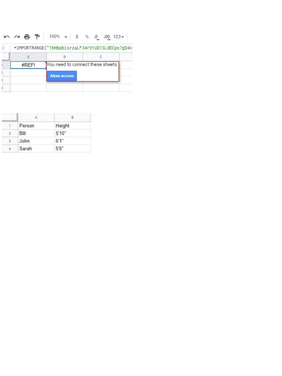
You’ll notice that attempting to use this formula, assuming you’ve properly replaced

spreadsheet_url, will initially show a reference error. You’ll need to then click on the cell to connect

these two sheets.

If everything has been done correctly, you should now see the data imported into your current sheet.

Simple, right? It’s worth noting that formatting will not be preserved during this import, as you can

see above, but all of the plaintext data will be.

Why Use IMPORTRANGE?

Now that you see how easy it is to use IMPORTRANGE, why would you ever use it? Let’s go over a few

quick example use cases.

Better Organization

You may find yourself involved in a very complex sheet that has moving variables that you want to

separate completely from other parts of your data. IMPORTRANGE is perfect for this, as it allows you

to do just that.

Since IMPORTRANGE easily allows you to import data from another worksheet within the same

spreadsheet, you can create a “Variables” worksheet where you can store anything with moving

parts. A combination of IMPORTRANGE, QUERY, and CONCATENATE could then be used to bring

everything together.

Collaborating With a Friend

Two heads are better than one, and IMPORTRANGE will even allow you to connect to sheets that your

account doesn’t own, as long as it’s shared with you. If you’re working on a collaborative project, the

work of two or more people can be dynamically consolidated into a single sheet using

IMPORTRANGE.

Hiding Sensitive Data

If you have a private spreadsheet with rows or columns that you want to show publicly,

IMPORTRANGE is great for that.

One example would be if you were to create a form with Google Forms. In it, you may ask for some

of the respondents’ personal information—you obviously don’t want to give that out, right? However,

the form may also ask less personal questions that you want to display in a public shared link. By

setting the range_string accordingly and connecting the form’s response sheet, this can be achieved.

Article courtesy of: https://helpdeskgeek.com/how-to/how-to-import-data-into-google-sheets-

from-another-sheet/