
Lecture Note 5: Price Discrimination
Imagine you are in charge of Disneyland’s pricing division.
• Congratulations! ECN 100B has served you well.
Your mission: pick the ticket price p to maximize profits.
• Write the profit function, take the FOC, set MR = MC .
• End up with p
m
= $100 and Q
m
= 50,000 visitors per day.
• Lots of profit, lots of consumer surplus. Everybody wins!
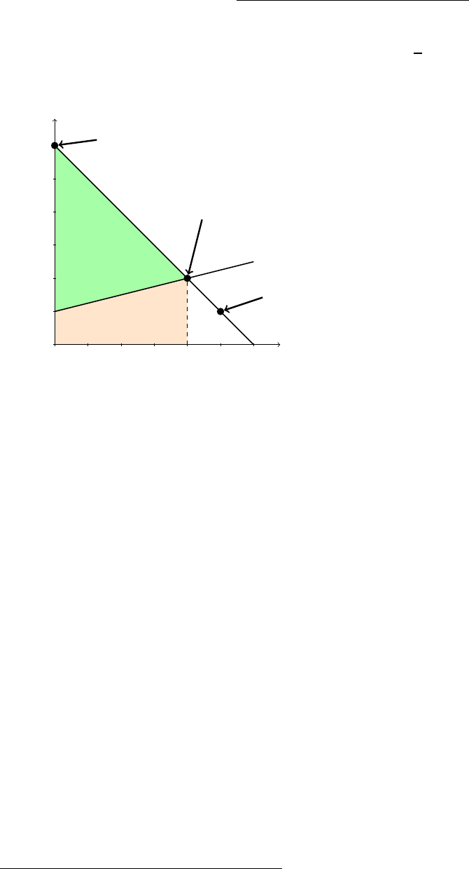
p
Q
p(Q)MR(Q)
MC (Q)
p
m
= 100
Q
m
= 50,000
• Green: producer surplus
• Blue: consumer surplus
(people who’d pay > $100)
• Gray: DWL (people who’d pay
more than MC but < $100)
But something is bugging you . . .
• Lots of people would pay over $100. Can we charge them more?
• Lots of people won’t pay $100. Should we charge them less?
Can we turn the CS and DWL into even more profit?
Copyright
c
2019 by Brendan M. Price. All rights reserved. 1

Types of pricing practices
uniform pricing: charging the same price for every unit you sell.
• Example: a gas station charges $3.75 per gallon of gas, no matter
who you are, no matter how many gallons you buy.
price discrimination: charging different per-unit prices for the same
product, depending on who is buying it or on how many units they buy.
Economists subdivide price discrimination into three categories.
1
personalized pricing: a firm offers each consumer her own individual
price. We’ll focus on an extreme form called perfect price discrimination.
• Contractors (e.g., exterminators) give their clients personalized prices.
• So do car dealerships.
group pricing: a firm charges different prices to different groups of
customers, but the same price for all members of each group.
• Disneyland gives SoCal residents a better deal.
• Comcast gives a low “teaser” rate to new subscribers.
nonlinear pricing: the unit price depends on the quantity purchased.
• Most consumer goods are cheaper if you purchase in bulk.
• Your first Netflix show costs you $12.99. The rest are free.
We’ll restrict our attention to perfect and group price discrimination.
1
Perfect, nonlinear, and group pricing are also called first-, second-, and third-degree price
discrimination, respectively. Firms often combine them: e.g., Disneyland charges lower admission
fees for SoCal residents (group pricing), but it also gives multi-day discounts (nonlinear pricing).
Copyright
c
2019 by Brendan M. Price. All rights reserved. 2

The gold standard: perfect price discrimination
Perfect price discrimination is a form of personalized pricing in which a
firm sells each unit at the maximum price that the consumer will accept.
• Not only does the firm charge each buyer her own individual price—
it charges her exactly her reservation price (willingness to pay).
Suppose that Davis Chevrolet can buy 2020 Chevy Malibus at a constant
(marginal) cost of $20,000 per car. Also suppose that they have top-notch
salespeople who can tell
exactly how much each customer is willing to pay.
Let’s consider three different customers:
• Bonnie has just robbed a bank, and she is trying to get out of town.
She’s willing to pay $60,000 for a Chevy Malibu.
◦ The dealership should sell her a car for $60,000. The dealership
makes $40,000 in profit; Bonnie gets zero consumer surplus.
• Jisung would pay $10,000 for a Malibu. (He’d rather drive a hybrid.)
◦ They’ll never be able to make a deal. Any price that Jisung
would accept would generate negative profit for the dealership.
• Luu would pay $20,000 for a Malibu. (After all, it’s a decent car.)
◦ It doesn’t really matter. The only price they’d both accept is
$20,000, which yields zero surplus for both parties.
We can extend these intuitions to analyze the entire market.
• Suppose the demand curve is p(Q) = 60 − Q.
The demand curve ranks consumers by their WTP for the good.
• Suppose that the marginal cost curve is MC (Q) = 10 +
1
4
Q.
This ranks items by the cost of producing/supplying them.
Copyright
c
2019 by Brendan M. Price. All rights reserved. 3
The Malibu market
With p(Q) = 60 − Q and MC (Q) = 10 +
1
4
Q, the market looks like this:
p
Q
0 10 20 30 40 50 60
0
10
20
30
40
50
60
p(Q)
MC (Q)
Bonnie
Luu
Jisung
A
B
C
• Total revenue: A + B.
• Total (variable) costs: B.
• Profit is revenue − cost: A.
The firm decides what price to offer each consumer, one at a time:
• If p(Q) > MC (Q): charge customer Q the price p(Q).
2
• If p(Q) < MC (Q): refuse to sell. (We can also think of this as the
firm charging MC (Q), knowing that the consumer will walk away.)
• If p(Q) = MC (Q): either charge p(Q) or refuse to sell. (It doesn’t
really matter whether this marginal transaction happens or not.)
Let’s do our usual welfare analysis—calculating everybody’s surplus:
• CS = 0 (because each consumer is charged their reservation price).
• PS = 1000 (which equals the total surplus under perfect comp).
• DWL = 0 (there are “no missed opportunities” to make a deal).
We get the Pareto efficient outcome . . . but the firm extracts all the surplus.
2
We’re assuming here that, if the customer is indifferent, he buys the car. This assumption isn’t
very important: the dealership could always charge him p(Q) − ε, where ε is negligibly small. The
customer would accept this deal and the dealership would make essentially the same profit.
Copyright
c
2019 by Brendan M. Price. All rights reserved. 4

Group price discrimination
Most firms don’t try to charge every customer their own price. And the
ones that do are unlikely to achieve truly “perfect” price discrimination.
The main reason is that doing so requires a ton of information.
3
• A uniform-pricing monopolist just needs to know how many units it
can sell at any given price—what does the demand curve look like?
• A perfect price discriminator has to know every consumer’s WTP—
the identity of the customer at each point on the demand curve.
• Some sellers (e.g., pawn shops) charge each buyer a different price,
based on their best guess of what price she’ll accept. But even good
salespeople usually can’t extract all of the surplus from a trade.
4
But firms engage in group price discrimination all the time.
• Movie theaters give discounts for students, seniors, and veterans.
• UC Davis charges vendors more than visitors for parking.
Disneyland sells tickets to SoCal residents and NorCal residents.
• SoCal demand = p
S
(Q
S
).
• NorCal demand = p
N
(Q
N
).
Disneyland’s costs depend on its sales to both groups: C(Q
S
, Q
N
).
The cost of an extra visitor probably doesn’t depend on where she’s from,
so let’s assume that costs are C(Q
S
+ Q
N
): they just depend on the sum.
What price should we charge each group? Should we price discriminate?
3
There are other reasons. Price discrimination only works if firms can prevent “resale” from
customers with big discounts to customers that face high prices. In some contexts, consumers may
view price discrimination as unfair and switch to other sellers. Certain forms of price discrimination
(e.g., charging different prices based on a customer’s race) are illegal under US law.
4
Big data may be changing this, by enabling tech firms to better guess buyers’ reservation prices.
Copyright
c
2019 by Brendan M. Price. All rights reserved. 5

Maximizing profits with two groups
As always, let’s start by writing the profit maximization problem:
max
Q
S
,Q
N
π(Q
S
, Q
N
) = R
S
(Q
S
) + R
N
(Q
N
) − C(Q
S
+ Q
N
)
Calculus tells us that we need to take one FOC for every choice variable.
Partially differentiating profits with respect to Q
S
yields the FOC for Q
S
:
∂π(Q
S
, Q
N
)
∂Q
S
= MR
S
(Q
S
) −
∂
∂Q
S
C(Q
S
+ Q
N
) = 0
Let’s define Q = Q
S
+ Q
N
. Using the chain rule,
∂
∂Q
S
C(Q
S
+ Q
N
) = C
0
(Q
S
+ Q
N
)
∂(Q
S
+ Q
N
)
∂Q
S
= C
0
(Q) · 1 = MC (Q)
So we can write the FOC for Q
S
as
MR
S
(Q
S
) = MC (Q)
Likewise, we can write the FOC for Q
N
as
MR
N
(Q
N
) = MC (Q)
Putting it all together, Disneyland chooses Q
S
and Q
N
to satisfy
MR
S
(Q
S
) = MR
N
(Q
N
) = MC (Q)
To gain intuition for optimality conditions like these, it’s helpful to start
at the wrong answer and look for a profitable deviation.
• Example 1: suppose that MR
S
(Q
S
) > MR
N
(Q
N
).
Raise Q
S
by δ, lower Q
N
by δ. Revenue rises, costs same =⇒ π ↑.
• Example 2: suppose that MR
S
(Q
S
) < MC (Q).
Lower Q
S
by δ. Revenue falls, but costs fall even more =⇒ π ↑.
Unless both FOCs hold, we aren’t optimizing: there’s a way to do better.
Copyright
c
2019 by Brendan M. Price. All rights reserved. 6

A numerical example
Suppose that . . .
• SoCal’s (inverse) demand is p
S
(Q
S
) = 90 − Q
S
• NorCal’s (inverse) demand is p
N
(Q
N
) = 180 − 2Q
N
• Costs are C(Q
S
, Q
N
) = 60Q
S
+ 60Q
N
Disneyland maximizes profits:
max
Q
S
,Q
N
π(Q
S
, Q
N
) = (90 − Q
S
)Q
S
| {z }
R
S
(Q
S
)
+ (180 − 2Q
N
)Q
N
| {z }
R
N
(Q
N
)
−60Q
S
− 60Q
N
FOC for Q
S
:
∂π
∂Q
S
= 90 − 2Q
S
− 60 = 0 =⇒ Q
∗
S
= 15, p
∗
S
= 75
FOC for Q
N
:
∂π
∂Q
N
= 180 − 4Q
N
− 60 = 0 =⇒ Q
∗
N
= 30, p
∗
N
= 120
This example is a bit special: because each FOC just depends on a single
choice variable, we can solve the system of equations one line at a time.
What this means is that—in this example—Disneyland’s optimal choice of
how many tickets to sell to SoCal residents doesn’t depend on how many
tickets it plans to sell to NorCal customers. It’s as though Disneyland is
running two separate businesses—one for SoCal and one for NorCal.
We can see this if we rearrange the profit equation:
π(Q
S
, Q
N
) = (90 − Q
S
)Q
S
− 60Q
S
| {z }
profits from SoCal customers
+ (180 − 2Q
N
)Q
N
− 60Q
N
| {z }
profits from NorCal customers)
In most cases, however, it’s impossible to split up profits like this, and we
will have to jointly solve the full system of equations.
5
5
For example, suppose Disneyland’s costs are C(Q
S
, Q
N
) = (Q
S
+ Q
N
)
2
= Q
2
S
+ 2Q
S
Q
N
+ Q
2
N
.
The interaction term 2Q
S
Q
N
depends on both SoCal and NorCal ticket sales. This creates a link
between the two choice variables, and Disneyland will have to choose them simultaneously.
Copyright
c
2019 by Brendan M. Price. All rights reserved. 7

The price-sensitive group gets a better deal
SoCal: p
S
(Q
S
) = 90 − Q
S
p
S
Q
S
0 15 30 45 60 75 90
0
60
75
90
120
180
p
S
(Q
S
)
MR
S
(Q
S
)
MC (Q)
(Q
∗
S
, p
∗
S
)
NorCal: p
N
(Q
N
) = 180 − 2Q
N
p
N
Q
N
0 15 30 45 60 75 90
0
60
75
90
120
180
p
N
(Q
N
)
MR
N
(Q
N
)
MC (Q)
(Q
∗
N
, p
∗
N
)
What can we learn from Disneyland’s pricing behavior?
• SoCal markup:
75−60
60
= 25%. NorCal markup:
120−60
60
= 100%.
• Recall that price markups are bigger when consumers are less elastic.
• For SoCal, −
1
1+ε
S
= 25% =⇒ ε
S
= −5.
• For NorCal, −
1
1+ε
N
= 100% =⇒ ε
N
= −2.
SoCal customers are more elastic, and they face a lower markup.
This is the key point about group price discrimination: groups that are
more price-sensitive get a better deal. Intuitively, the firm knows it can’t
rip them off: if it charges too much, price-sensitive consumers walk away.
Group pricing lets a firm “segment the market”, charging each group a
price tailored to its willingness to pay. Many real-world pricing strategies
are designed to segment the market in this manner, giving discounts to
price-sensitive consumers and charging high prices to the inelastic ones.
Copyright
c
2019 by Brendan M. Price. All rights reserved. 8

Kinked demand curves
Recall that we obtain the market demand curve by adding up individual
consumers’ demand curves horizontally. We can do the same thing here,
taking the horizontal sum of the SoCal and NorCal demand curves.
The market demand curve looks like this:
p
Q
0 30 45 60 90 120 150 180
0
30
60
90
120
150
180
p(Q)
MC (Q)
This is a “kinked” demand curve, with a bend or “kink” at Q = 45.
Drawing kinked demand curves is a bit tricky. Let’s do it in two steps.
First, when the price is above 90, nobody from SoCal is willing to buy.
Therefore, for p > 90, the market demand curve lines up exactly with the
NorCal demand curve. That gets us from Q = 0 to Q = 45:
p(Q) = 180 − 2Q for Q < 45
Next, when the price is below 90, some consumers from both SoCal and
NorCal are willing to buy. To find out how many consumers in total are
willing to buy, we have to invert the two demand curves:
p
S
(Q
S
) = 90 − Q
S
=⇒ Q
S
(p
S
) = 90 − p
S
p
N
(Q
N
) = 180 − 2Q
N
=⇒ Q
N
(p
N
) = 90 −
1
2
p
N
Copyright
c
2019 by Brendan M. Price. All rights reserved. 9

If Disneyland charges both groups the same price p, then total demand is
Q(p) = Q
S
(p) + Q
N
(p) = 180 −
3
2
p
Inverting this equation, we obtain the market demand curve for p < 90,
or in other words for Q ≥ 45:
p(Q) = 120 −
2
3
Q for Q ≥ 45
Putting it all together, the market demand curve is defined piecewise by
p(Q) =
(
180 − 2Q for Q < 45
120 −
2
3
Q for Q ≥ 45
That’s the function I plotted in the graph above.
What if Disneyland were a uniform-pricing monopolist?
Let’s now imagine that Disneyland has to operate as a uniform-pricing
monopolist. (Perhaps a California state law has outlawed the practice of
charging different prices to families from different parts of the state.) Our
goal is to find the pair (Q
m
, p
m
) that maximizes Disneyland’s profits.
Unfortunately, the presence of the kink makes optimization a little more
difficult, because the profit function is not differentiable at Q = 45. To
find the optimal choice Q
m
, here’s what we have to do:
1. Maximize profits as if demand were p(Q) = 180 − 2Q for all Q.
We get a candidate solution Q
m
= 30, p
m
= 120, with π = 1800.
2. Maximize profits as if demand were p(Q) = 120 −
2
3
Q for all Q.
We get a candidate solution Q
m
= 45, p
m
= 90, with π = 1350.
3. We now have two candidate solutions. Picking the one that yields
higher profits gives us the final answer: Q
m
= 30, p
m
= 120.
Copyright
c
2019 by Brendan M. Price. All rights reserved. 10

So, if Disneyland has to charge everybody the same price, we get this:
p
Q
0 30 45 60 90 120 150 180
0
30
60
90
120
150
180
p(Q)
MC (Q)
(Q
m
, p
m
)
This solution reveals some important insights:
1. Is price discrimination profitable? As a uniform-pricing monopolist,
Disneyland would make profit of π = 1800. Under group price
discrimination, Disneyland makes extra profit: π = 2025.
This is a general insight: engaging in price discrimination allows
firms to increase their profits. We’ll come back to this shortly.
2. Under group price discrimination, Disneyland sells tickets to both
SoCal and NorCal customers. Under uniform pricing, it “gives up”
on SoCal: at the uniform price p
m
= 120, nobody from SoCal buys.
Because SoCal residents have much lower WTP than people from
NorCal, the only way Disneyland can attract SoCal customers is by
lowering the price a lot. Under uniform pricing, Disneyland would
have to give a big discount to NorCal, too, and that’s not worth it.
The lesson here is that, when firms have to charge everybody the
same price, they sometimes just sell to the top end of the market.
Group price discrimination gets them to service the low end, too.
Copyright
c
2019 by Brendan M. Price. All rights reserved. 11

3. Price-sensitive groups tend to benefit from group pricing because
firms typically give them discounted prices. In this example, SoCal
residents get consumer surplus under group price discrimination, but
not under uniform pricing.
4. Price-inelastic groups are generally worse off under group pricing
because firms typically charge them higher prices. That doesn’t
happen in this example, but in the real world Disneyland probably
charges NorCal customers more than it would under uniform pricing.
5. Group pricing sometimes reduces the monopoly deadweight loss by
getting monopolists to service segments of the market they would
otherwise ignore. (Sometimes, however, group pricing raises DWL.)
Revealed preference
I want to conclude by revisiting the question of whether the ability to
engage in price discrimination increases Disneyland’s profits.
We calculated profits under both uniform and group pricing, and we found
that group pricing yields higher profit. But there’s a simpler argument:
• Under group pricing, Disneyland could have chosen p
S
= p
N
.
• But they didn’t: they maximized profits with p
S
6= p
N
.
• Thus, uniform pricing (p
S
= p
N
) would have yielded lower profits.
• The ability to price discriminate can never lower a firm’s profits
(they can always choose not to do it) and usually raises their profits.
This elegant line of reasoning is called a revealed preference argument:
Disneyland’s behavior “reveals” that it benefits from price discrimination.
Whenever we see firms engage in price discrimination, we can safely assume
that it’s increasing their profits: otherwise they wouldn’t be doing it!
Copyright
c
2019 by Brendan M. Price. All rights reserved. 12
