I
NNOCENT
B
YSTANDERS
?
M
ONETARY
P
OLICY AND
I
NEQUALITY IN THE
U.S.
Olivier Coibion Yuriy Gorodnichenko
UT Austin
and NBER
U.C. Berkeley
and NBER
Lorenz Kueng John Silvia
Northwestern University
and NBER
Wells Fargo
This Draft: February 17
th
, 2016
Abstract: We study the effects of monetary policy shocks on—and their historical
contribution to—consumption and income inequality in the United States since 1980 as
measured by the Consumer Expenditures Survey. Contractionary monetary policy
systematically increases inequality in labor earnings, total income, consumption and total
expenditures. Furthermore, monetary policy shocks account for a non-trivial component
of the historical cyclical variation in income and consumption inequality. Using detailed
micro-level data on income and consumption, we document some of the different
channels via which monetary policy shocks affect inequality, as well as how these
channels depend on the nature of the change in monetary policy.
Keywords: Monetary policy, income inequality, consumption inequality.
JEL codes: E3, E4, E5.
The authors acknowledge the financial support of the Global Interdependence Center and are grateful to
Stefania Albanesi, Jihad Dagher, Pierre Jaillet, Ricardo Reis, Aysegul Sahin and anonymous referees for
comments. We thank Peter Ireland for sharing his data. The views in the paper are those of the authors
and do not necessarily represent those of Wells Fargo.
1
I Introduction
With the level of income inequality in the U.S. rising to record levels in recent years, popular
concern with this question has grown, as illustrated for example by the Occupy Wall Street
movement. The topic of inequality has even breached the walls of the central banking community,
and a number of monetary policymakers have departed from their traditional focus on aggregate
considerations to discuss the potential distributional effects of monetary policy actions (Mersch 2014,
Bullard 2014, Forbes 2015, Bernanke 2015). But how even typical monetary policy decisions, much
less quantitative easing or forward guidance, affect economic inequality is a priori ambiguous
because of the number of channels through which these actions affect agents. In this paper, we show
that contractionary monetary policy shocks by the Federal Reserve have historically been followed
by persistent increases in income and consumption inequality and provide evidence on some of the
channels underlying these distributional consequences of monetary policy.
One channel that can generate heterogeneous effects of monetary policy on income is the
income composition channel, i.e. the fact that there is heterogeneity across households in terms of their
primary sources of income. While most households rely primarily on labor earnings, others receive
larger shares of their income from business, financial or transfer income. To the extent that monetary
policy affects these different forms of income in a heterogeneous manner (and it does), then different
types of households will experience different income outcomes. For example, richer households tend to
receive relatively more business income, and since the latter tends to rise relative to wages after
expansionary monetary shocks, this effect would tend to increase income and consumption inequality.
A second channel is the financial segmentation channel: if some agents frequently trade in financial
markets and are affected by changes in the money supply prior to other agents, then an increase in the
money supply will redistribute wealth toward those agents most connected to financial markets, as in
Williamson (2009) and Ledoit (2009). If agents participating actively in financial trades have higher
income and consumption on average than unconnected agents, then this channel implies that
consumption inequality should rise after expansionary monetary policy shocks. An additional channel
pushing in the same direction is the portfolio channel. If low-income households tend to hold relatively
more currency than high-income households (Erosa and Ventura 2002, Albanesi 2007), then
inflationary actions on the part of the central bank would represent a transfer from low-income
households toward high-income households which would tend to increase consumption inequality.
Two other channels, however, will tend to move inequality in the opposite direction in response
to expansionary monetary policy actions. The first is the savings redistribution channel: an unexpected
increase in interest rates or decrease in inflation will benefit savers and hurt borrowers as in Doepke
2
and Schneider (2006), thereby generating an increase in consumption inequality (to the extent that
savers are generally wealthier than borrowers). The second is the earnings heterogeneity channel.
Labor earnings are the primary source of income for most households and these earnings may respond
differently for high-income and low-income households to monetary policy shocks. This could occur,
for example, if unemployment disproportionately falls upon low income groups, as documented in
Carpenter and Rogers (2004). Similar effects could arise among the employed due to different wage
rigidities across the income distribution (e.g. from unionization in production but not management),
varying degrees of complementarity/substitutability with physical capital depending on agents’ skill
sets, or different endogenous labor supply responses from household-specific characteristics which
differ across the distribution. Heathcote et al. (2010), for example, document that the labor earnings at
the bottom of the distribution are most affected by business cycle fluctuations. The income composition
channel could also push toward reduced—rather than increased—inequality after expansionary
monetary policy since low-income households receive, on average, a larger share of their income from
transfers (e.g. unemployment benefits, food stamps) and transfers tend to be countercyclical.
In short, these different channels imply that the effect of monetary policy on economic
inequality is a priori ambiguous. As a result, we turn to the data to assess whether U.S. monetary
policy has contributed to historical changes in consumption and income inequality in the U.S., and if
so, through which channels. To do so, we study the dynamic responses of measures of consumption
and income inequality to monetary policy shocks identified as in Romer and Romer (2004). Our
measures of inequality come from detailed household-level data from the Consumer Expenditures
Survey (CEX) since 1980. These data are available on a higher frequency (quarterly) than other
sources such as IRS data employed by Piketty and Saez (2003), which is necessary to analyze the
effects of monetary policy shocks. While the CEX does not include the very upper end of the income
distribution (i.e. the top 1%) which has played a considerable role in income inequality dynamics
since 1980 (CBO 2011), the detailed household-level data do allow us to consider a wide range of
inequality measures for labor income, total income, consumption and total expenditures.
Using these measures of inequality, we document that monetary policy shocks have
statistically significant effects on inequality: a contractionary monetary policy shock raises the
observed inequality across households in income, labor earnings, expenditures and consumption.
These results are robust to the time sample, such as dropping the Volcker disinflation period or all
recession quarters, with only earnings inequality displaying some sensitivity. They are also largely
invariant to controlling for household size and other observable household characteristics such as
age, education and family size. The effects are economically large for consumption and expenditure
3
inequality, and moderate for total income inequality, but the effects on earnings inequality are much
smaller. Given the historical sequence of identified monetary policy shocks, these shocks appear to
have played a non-trivial role in accounting for cyclical fluctuations in some forms of inequality over
this period. While the contribution of monetary policy shocks to labor earnings inequality is virtually
nil in forecast error variance decompositions, it is approximately 10 percent for total income at
longer horizons and over twenty percent for consumption and expenditure inequality. Furthermore,
monetary policy shocks can account for a surprising amount of the historical cyclical changes in
income and expenditure inequality, particularly since the mid-1990s.
The fact that overall labor earnings inequality responds little to monetary policy shocks masks
some underlying distributional heterogeneity. After a contractionary monetary policy shock, upper
income households (90
th
percentile) see their labor incomes rise on average relative to the median
household, but so do low income households (10
th
percentile), at least temporarily. This leads to a
widening of the earnings distribution at the upper tail but a condensing of the distribution at the lower
tail, i.e. the earnings distribution becomes more skewed as in Guvenen et al. (2014). There is therefore
evidence for the earnings heterogeneity channel, even though its effects on the second moments of the
distribution are very small.
The effects of monetary policy shocks on total income inequality are larger, a feature which
appears to primarily reflect the income composition channel. We find that the incomes of households
at the 90
th
percentile rise somewhat relative to the median household, while households at the 10
th
percentile see their relative incomes fall particularly sharply. This is consistent with the fact that low
income households receive a much larger share of their income from transfers than labor earnings
than other groups, and real wages rise relative to transfers after monetary shocks. We also find that
financial income rises sharply after monetary policy shocks. Because the top 1% of the income
distribution receive a disproportionate share of their income from financial income (CBO 2011), our
baseline results on income inequality are most likely a lower bound since they exclude the top 1%.
The effects on consumption and expenditure inequality are larger still. But unlike the
heterogeneity in income inequality, heterogeneity in consumption and expenditure is driven primarily
by the upper end of the distribution: those at the 90
th
percentile see a much larger rise in consumption
and expenditures relative to the median household than the relative decline seen by those at the 10
th
percentile. In fact, the relative changes in consumption at the upper end of the distribution are
significantly larger than their relative changes in income, which suggests that portfolio, savings
redistribution and/or financial segmentation channels must also play some role.
4
Because the CEX does not include reliable measures of household wealth, it is difficult to
identify these channels. For example, in the absence of consistent measures of the size of household
currency holdings or financial market access in the CEX, we cannot directly quantify the specific
(money holding) portfolio channel emphasized by Albanesi (2007) or the financial market
segmentation channel in Williamson (2009). Nonetheless, to the extent that both channels imply that
contractionary monetary policy shocks should lower consumption inequality, the fact that our baseline
results go in the opposite direction suggests that these channels, if present, must be relatively small.
However, in the case of the savings redistribution channel, we provide evidence of wealth transfers by
identifying high and low net-worth households following the characterization of Doepke and Schneider
(2006), namely that high net-worth households are older, own their homes, and receive financial
income while low net-worth households are younger, have fixed-rate mortgages and receive no
financial income. We find that while the average responses of total income and labor earnings are
broadly similar across the two groups, consumption and, to a lesser extent, total expenditures rise
significantly more for high net-worth households than low net-worth households after contractionary
policy shocks.
Finally, we consider the sensitivity of these results to the nature of the monetary policy
innovation. Specifically, we focus on changes in the Fed’s inflation target, identified either as in
Coibion and Gorodnichenko (2011) or as in Ireland (2006). Permanent decreases in the inflation target
are also associated with higher levels of labor earning, total income, expenditure and consumption
inequality. While historical changes in the Fed’s inflation target account for a smaller fraction of the
forecast error variance than broader measures of monetary shocks for each form of inequality, changes
in the inflation target can account for the vast majority of the dynamics of inequality over the early to
mid-1980s, indicating that the Volcker disinflation period likely played a particularly important role in
accounting for the evolution of economic inequality during this time period.
Monetary policy therefore may well have played a more significant role in driving recent
historical inequality patterns in the U.S. than one might have expected. These results are noteworthy
for several reasons. First, the potential contribution of monetary policy to inequality has received
relatively little attention in the economics literature (Romer and Romer (1998) is an early exception).
Understanding and quantifying the sources of inequality is a first step to determining what kinds of
policies, if any, are most appropriate to address it. Second, the heterogeneity in consumption and
income responses across households, as well as the channels underlying them, are of immediate
relevance to monetary economists and policymakers for understanding the monetary transmission
mechanism. In addition, some research has linked rising inequality to credit booms and financial

5
crises (e.g. Rajan 2010, Kumhof et al. 2015), therefore suggesting a potential link from inequality to
macroeconomic stability. Third, there is a growing macroeconomics literature integrating
heterogeneous agents and distributional effects into New Keynesian models to revisit optimal fiscal
and monetary policy design.
1
Our results provide a rich set of stylized facts about the conditional
responses of income, earnings and consumption patterns across households to monetary policy shocks
that can be used to calibrate and differentiate between different classes of heterogeneous agent
models, in the same spirit as the use of monetary policy shocks by Christiano et al. (2005) to estimate
the parameters of New Keynesian models. Finally, recent work (e.g. Heathcote et al. 2010) has
emphasized not only the cyclical component to economic inequality but also the variation in
inequality across business cycle episodes. With changes in monetary policy having been proposed as a
potential contributor to the Great Moderation (e.g. Clarida et al. 2000), one can naturally consider
monetary policy as also affecting cyclical inequality patterns.
The paper is structured as follows. Section 2 discusses the Consumer Expenditure Survey, the
construction of inequality measures and their unconditional properties. Section 3 presents the main
results on the effects of monetary policy shocks on income, labor earnings, expenditure and
consumption inequality. Section 4 assesses the wealth effects of monetary policy shocks while
section 5 considers the implications of changes in the inflation target. Section 6 concludes.
II Measuring Inequality
In this section, we briefly describe the Consumer Expenditure Survey and the construction of
measures of inequality for total income, wage income, consumption and total expenditures.
2.1 The Consumer Expenditure Survey
The Consumer Expenditure Survey (CEX) is the most comprehensive data source on household
consumption in the U.S. and is used for constructing weights of the Consumer Price Index (CPI). The
CEX, which is provided by the Bureau of Labor Statistics (BLS), consists of two separate surveys:
the Interview Survey and the Diary Survey. In this study we only use data from the Interview Survey
since the Diary Survey covers only expenditures on small items that are frequently purchased, mostly
related to food. The Interview Survey provides information on up to 95% of the typical household's
consumption expenditures. The CEX is a monthly rotating panel, where households are selected to be
representative of the US population, and is available on a continuous basis since 1980. About 1,500-
1
Examples include Gornemann et al. (2014), Guerrieri and Lorenzoni (2015), Luetticke (2015), Auclert (2016),
Kaplan et al. (2016), and McKay and Reis (2016).

6
2,500 households are surveyed in any given month. Each household is interviewed once per quarter,
for at most five consecutive quarters, although the first interview is used for pre-sampling purposes
and is not available for analysis. In each interview, the reference period for expenditures covers the
three months prior to the interview month. However, the within-interview variation is much lower
than the between-interview variation because the BLS processes many individual expenditure
categories assigning a third of the reported spending to each of the three months. Moreover, many
households also seem to smooth their reported three-month expenditures equally over the three
months. While these three-monthly periods do not coincide with calendar quarters and monthly
spending can include information from periods outside a given calendar quarter, we aggregate
monthly expenditures into quarterly expenditures to maximize the size of the sample and thus reduce
sampling error in the resulting series as well as to make the resulting series conformable with other
macroeconomic variables. In robustness checks, we explore alternative aggregation approaches and
find similar results. In short, “household time” is quarterly.
We define household consumption as the sum of non-durables (e.g. food and gasoline),
services, and expenditures on durable goods (e.g. furniture, jewelry). We also construct a broader
measure of household expenditures by adding mortgage and rent payments, health expenditures,
education spending and other expenses to household consumption levels.
2
As recommended by the
BLS, we sum expenditures that occur in the same month but are reported in different interviews.
Income data is asked in the first and last interview, and financial data is only asked in the last interview.
The reference period for income flows covers the twelve months before the interview. All nominal
variables are deflated using the CPI-U and survey sample weights are consistently applied. To reduce
the influence of outliers, we winsorized income and spending variables at bottom and top 1 percent.
3
Much work has been devoted to assessing the quality of the CEX relative to other data.
Heathcote et al. (2010), for example, compare income inequality data in the CEX with equivalent
measures from the Panel Study of Income Dynamics (PSID) and the Current Population Survey
(CPS). They find strong comovement among pre-tax earnings inequality measures from all three
surveys. Attanasio (2003) and Attanasio et al. (2004) similarly document the consistency of wage
inequality in the CEX and the CPS. More concern has been raised with respect to underreporting of
2
We correct sample breaks due to slight changes in the questionnaire of the following variables: food at home
(1982Q1-1988Q1), personal care services (2001Q2), and occupation expenditures (2001Q2). To further improve the
quality of the data, we drop the following observations: interviews with more or less than three monthly
observations; households reporting zero food or total expenditures; and observations with negative expenditures
where there should not be any.
3
See Appendix B for more details on how we process CEX data.

7
consumption in the CEX. For example, Krueger et al. (2010), Aguiar and Bils (2015) and Attanasio
et al. (2012) document that the CEX underreports consumption relative to aggregate data and that
this underreporting has become more severe over time. On the other hand, Bee et al. (2012) compare
reported consumption spending data in the CEX to comparable data from the national income
accounts data and find that the CEX data conform closely to aggregate data for large consumption
categories. For our purposes, the potential underreporting of consumption in the CEX is less of a
concern, since we will focus on cyclical fluctuations in consumption inequality. In addition, our
empirical specifications will focus on changes in inequality rather than levels. Nonetheless, the
potential limitations in the quality of the CEX survey data are an important caveat to bear in mind.
2.2 Measures of Inequality
Given the availability of household data on both consumption and income, the CEX allows us to
study the behavior of both forms of inequality. To do so, we focus on three ways of measuring each
form of inequality: Gini coefficients of levels, cross-sectional standard deviations of log levels, and
differences between individual percentiles of the cross-sectional distribution of log levels.
4
The Gini
coefficient has long been used to measure inequality and summarizes the extent to which a variable is
equally allocated across different components of the distribution. In addition, we will also use the
cross-sectional standard deviation of log values. Taking logs diminishes the sensitivity to outliers but
requires us to drop observations equal to zero, in contrast to the Gini coefficient. Finally, we use the
difference between the 90
th
percentile and the 10
th
percentile of the log levels in each distribution,
which also requires the elimination of observations with values of zero. However, the percentile
differential is less sensitive to extreme observations in the tails of the distributions.
Given the detailed data in the CEX, we will consider two forms of inequality for income and
consumption each. On the income side, we first construct measures of labor earnings inequality
across households. Given the survey nature of the data, the advantage of labor earnings is that they
are likely to be known with the highest precision by households relative to other forms of income.
The disadvantage is that labor income is only one component of most households’ income. As a
result, we also construct measures of total income inequality based on labor earnings as well as
4
All of our baseline measures of inequality are raw, i.e. do not control for any household characteristics like the
number of household members, age, education, etc. This is because some of the channels by which monetary policy
might affect inequality could be systematically related to some of these observables. For example, the redistribution
of wealth from borrowers to savers should likely be related to the age of households. Controlling for age would
make it more difficult to identify this kind of channel. Similar logic applies to other household characteristics.
However, while our baseline measures do not control for any household observables, we consider a number of
robustness checks in which we do control for household characteristics.

8
financial income, business income and transfers for each household. Because individuals in the CEX
are asked about their income only in the first and last quarters of their participation in the survey and
the BLS imputes income for periods in between, we use only those individuals who are reporting
their income in each survey to construct measures of income and earnings inequality. Hence, the
sample used to construct income inequality measures each quarter is only a subset of the total
population in the survey that period. We will focus primarily on pre-tax measures of total income,
although we also present after-tax income inequality measures and show that our results are robust to
this alternative measure.
5
Appendix Table 1 reports correlations among the different measures of
inequality for both income and labor earnings: all correlations are quite high, with those for income
being 0.89 or above over the entire sample from 1980Q1 to 2008Q4.
Similarly, we construct both a narrow and broad measure of consumption inequality. The
narrow measure, which we refer to as consumption inequality, includes the same categories as in
Parker (1999). Consumption goods in this category include non-durables, services, and some durable
goods (household appliances, entertainment goods like televisions, furniture) but do not include large
durable purchases such as house and car purchases. We also define a broad measure of consumption,
which we refer to as total expenditures and which includes the previous definition of consumption as
well as mortgage payments, purchases of cars, medical supplies and services, and tuition and books
for schooling among others. In contrast to income measures, consumption and expenditure data for
individuals in the survey is measured every survey wave, so consumption and expenditure inequality
measures use the entire population in the survey each period subject to the caveats discussed in
section 2.1. For both consumption and expenditures, we aggregate all reported purchases within each
definition at the household level, then construct inequality measures across households. Appendix
Table 1 documents high correlations across measures of expenditure inequality, ranging from 0.75 to
0.89. Correlations among the consumption measures are slightly smaller, ranging from 0.79 to 0.43.
2.3 Unconditional Properties of Inequality Measures
Figure 1 plots the historical inequality measures of income, labor earnings, expenditures and
consumption inequality measures from the CEX based on the cross-sectional standard deviation
(Panel A), Gini coefficient (Panel B) and the 90
th
to 10
th
percentile differential (Panel C), averaged
over the previous and subsequent quarter to illustrate more clearly business cycle and low-frequency
variations. Consistent with results documented in the literature (Krueger and Perri 2005), our
5
Following Kueng (2012) we compute tax burdens using the TAXSIM calculator of the NBER; see Feenberg and
Coutts (1993). The code is available at http://www.nber.org/~taxsim/to-taxsim/cex-kueng.

9
measures of total income inequality are all trending up over time. A similar pattern occurs for labor
earnings inequality when measured using the Gini coefficient but not when measured using the cross-
sectional standard deviation nor the 90
th
– 10
th
percentile differential, a feature of the data also
documented in Heathcote et al. (2010). There is a sharp increase in all forms of inequality in the early
1980s. Income inequality rises over the course of the 1990s but not consumption or expenditure
inequality measures. Finally, there is a noticeable decline in expenditure inequality over the course of
the 2000s despite there being no such decrease in income inequality.
The figures therefore reveal some evidence of cyclical behavior in inequality measures,
consistent with Heathcote et al. (2010). Table 1 presents unconditional correlations between
inequality measures and quarterly inflation, the unemployment rate and the Federal Funds rate. All
series are HP-filtered prior to measuring correlations so that the latter primarily reflect business cycle
fluctuations rather than trends. Correlations of different forms of inequality with the inflation rate are
very small and somewhat negative. Similar results obtain with interest rate correlations. Labor
earnings inequality is weakly positively correlated with the unemployment rate and negatively with
inflation. Expenditure and consumption inequality are more strongly negatively correlated with the
unemployment rate. This could be interpreted as being consistent with a wealth channel, whereby
even if income inequality varies little with the business cycle, cyclical fluctuations in asset prices
have significant effects on wealth holdings of individuals, leading to lower consumption and
expenditures of the wealthy during recessions.
6
Overall, however, the unconditional correlations do
not point toward very strong links between business cycles and inequality patterns.
III Effects of Monetary Policy Shocks on Inequality
In this section, we present baseline results for the effects of monetary policy shocks on measures of
income inequality. We first discuss the construction of monetary policy shocks, then present results
quantifying the effects of these shocks on different forms of inequality in the U.S., as well as number
of robustness checks. We also present results on how monetary policy shocks affect different
components of the distributions, whether mobility within the distribution changes after monetary
shocks, and the economic importance of monetary policy for inequality dynamics.
3.1 The Identification of Monetary Policy Shocks
6
Consistent with this, Parker and Vissing-Jorgensen (2009) document that consumption of high-income households
moves disproportionately with aggregate consumption.
10
To characterize the effects of monetary policy (MP) on inequality in the U.S., we follow Romer and
Romer (2004, RR henceforth) to identify innovations to monetary policy purged of anticipatory
effects related to economic conditions. RR first construct a historical measure of changes in the target
Federal Funds rate (FFR) at each FOMC meeting from 1969 until 1996. Using the real-time forecasts
of the Fed staff presented in the Greenbooks prior to each FOMC meeting (denoted by F), RR
construct a measure of MP shocks from the component of policy changes at each meeting that is
orthogonal to the Fed’s information set. Specifically, they estimate
where m denotes the FOMC meeting,
is the target FFR going into the FOMC meeting,
is the Greenbook forecast from meeting m of real output growth in quarters around meeting
m (-1 is previous quarter, 0 is current quarter, etc.),
are Greenbook forecasts of GDP deflator
inflation, and
are Greenbook forecasts of the current quarter’s average unemployment rate.
The estimated residuals !
are then defined by RR as MP shocks.
We extend the RR dataset on MP shocks until December 2008 as follows. First, we
incorporate more recent changes in the target FFR decided upon at regular FOMC meetings. Second,
we extend the Greenbook forecasts until December 2008, the most recent period through which the
Federal Reserve has released them. The dataset therefore extends until the zero-bound on interest
rates became binding in December 2008. Estimating the exact same specification as RR upon this
extended dataset since January 1969 yields a sequence of MP shocks at the frequency of FOMC
meetings. We then construct a quarterly measure of MP shocks by summing the orthogonalized
innovations to the FFR from each meeting within a quarter. Consistent with the results documented
in RR, the shocks are particularly large and volatile in the early 1980s during the Volcker disinflation
(Appendix Figure 1). The shocks also identify periods in which policy was more contractionary than
usual conditional on real-time forecasts. For example, the “pre-emptive strike” against inflation in
1994-1995 is visible as a period of consistently positive MP shocks, as is the 2005-2006 period. The
2000-2004 period, on the other hand, is identified as more expansionary than would have been
typical given staff forecasts of macroeconomic conditions, consistent with Taylor (2007).
Before turning to the effects of MP shocks on inequality, we first investigate how
contractionary monetary policy actions affect macroeconomic aggregates, financial variables, as well as
more detailed income and consumption aggregates. We follow Jorda (2005) and estimate the response
of economic variables to monetary policy shocks at different horizons h using local projection methods

11
"
#$%
"
#$%
&
%
'
%
("
#'
"
#'
)
*
'
%
#
++,
--.-
#$%
/ 012
3
where x is the variable of interest and the
#
++
are quarterly monetary policy innovations. With the
exception of interest rates, we use first-differences of macroeconomic variables in estimating (2) and
generate accumulated impulse responses to MP shocks from the estimated 4
5
%
6
%
7
.
7
As a
benchmark, we set J=2 and I=20. We estimate the system of equations across horizons jointly.
Standard errors are as in Driscoll-Kraay (1998) to allow for arbitrary serial and cross-sectional across
horizons and time. For each impulse response, we present one and 1.65 standard deviation
confidence intervals, as well as p-values for tests of the null hypothesis that the impulse response is
equal to zero for all horizons / 012. We consistently use H=20 quarters.
The results are presented in Figure 2 using data from 1969:Q3 to 2008Q4, the entire period over
which MP shocks are available. For comparability across specifications, we define the time sample based
on the time series of the dependent variable for horizon h=0. Over the entire sample, contractionary
monetary policy shocks lower real GDP and raise unemployment, and lower consumption. The reduction
in consumption obtains for both durables as well as non-durables and services.
8
These results conform to
the empirical literature on the effects of MP shocks (see Christiano et al. 1999 for a review).
In addition, we consider the effects of MP shocks on real housing prices (Case-Shiller price
index deflated by the GDP deflator), which are a particularly important component of household
wealth. Real housing prices, the major financial asset for many households, decline gradually after one
to two years, ultimately falling by 5% after a one hundred basis point shock to the FFR. This suggests
one channel through which monetary policy might affect households differently: to the extent that
households’ wealth is not allocated in the same manner across assets, then those households whose
wealth is particularly concentrated in their home would tend to experience very different wealth effects
than non-homeowners. Wong (2015) presents additional evidence in line with this channel.
Figure 2 also presents responses of different sources of income to contractionary MP shocks.
The response of real wages is not statistically different from zero over either sample, while business
income drops rapidly and significantly. Financial income, on the other hand, rises significantly. Total
7
It is conventional to assume that monetary policy shocks do not have contemporaneous effects on output, inflation,
etc. but may have contemporaneous effect on interest rates, etc. Consistent with this convention, we set the
contemporaneous effect for all variables (except the fed funds rate) to zero in the impulse responses reported in Figure
2. That is, we use 8
5
%
9 rather than 8
5
%
9 for all variables but fed funds rate. For fed funds rate, we use 8
5
%
9.
8
NIPA’s definitions of spending are different from our definitions of consumption/spending in the CEX. NIPA’s
non-durable consumption is the closest counterpart of our definition of consumption in the CEX. Appendix Table 13
documents that the response of non-durable consumption is similar to the response of CEX-based measure of
consumption. Thus, although there is a discrepancy in the aggregate levels of CEX and NIPA spending, the impulse
responses to monetary policy shocks are not necessarily different.

12
income from transfers drops over the first year after a shock before returning to its original level. Thus,
these results suggest that heterogeneity in income sources across households may also lead to important
distributional consequences to monetary policy actions.
9
Contractionary monetary policy will tend to
raise incomes for those who receive a lot of financial income but lower incomes for business owners.
3.2 The Effects of Monetary Policy Shocks on Inequality
To quantify the overall effects of MP shocks on economic inequality, we estimate a version of
equation (2) using inequality measures for total income, labor earnings, total expenditure and
consumption, defined as in section 2:
10
"
#$%
"
#$%
&
%
'
%
("
#'
"
#'
)
*
'
%
#
++,
--.-
#$%
/ 012:
3;
Note that we allow a contemporaneous response of inequality to monetary policy shocks because of
time aggregation in the CEX data (we discuss this more below and in Appendix A) and thus the
impulse response is given by 4
5
%
6
%
7
.
We do so for each form of inequality using three different measures of inequality for each: the
cross-sectional standard deviation (of logged values), the Gini coefficient, and the difference between
the (log) 90
th
percentile and the (log) 10
th
percentile. While MP shocks are generated regressors, Pagan
(1984) shows that if the null hypothesis is
%
0 for any / 012, then standard errors need no
adjustment. Furthermore, as discussed in Coibion and Gorodnichenko (2012a), explicitly adjusting
standard errors for the presence of generated regressors has negligible effects in this setting because the
shocks are the residuals from the first stage rather than the fitted values. Given the consensus view
among mainstream economists that monetary policy has played little role in affecting economic
inequality in the U.S., this is a reasonable null to hold. Furthermore, because MP shocks are the residuals
from estimates of equation (1), they will be largely orthogonal to contemporaneous economic conditions
and other factors absorbed into the error term in equation (2), further justifying the use of unadjusted
standard errors. In estimating equation (2) for inequality measures, we consistently use a lag structure of
< 3 and = 30 quarters, but show later that our results are insensitive to alternative lag structures.
Figure 3 presents the accumulated impulse responses from estimates of equation (2) for each
form of inequality (income, labor earnings, expenditure and consumption) and measure of that
inequality (standard deviation, Gini, and 90
th
to 10
th
percentile differential) using data from 1980Q3
9
In Appendix Figure 2, we show that these differential responses of incomes also hold in the post-1980 period.
10
To ensure that changes in inequality are not driven by changes in the composition of CEX households over time,
we hold the set of households constant when we calculate changes in measures of consumption and expenditure
inequality from a given quarter to the next one.
13
until 2008Q4 and the associated one and 1.65 standard deviation confidence intervals. For each
response, we again report p-values for the test of the null hypothesis that monetary policy shocks
have no effect on each form of inequality across all (/ 0130) horizons. The results for both
income and labor earnings inequality point to statistically significant effects of MP shocks on
inequality. For total income inequality, the rise in inequality is somewhat delayed, occurring one to
two years after the shock depending on the specific measure. We can strongly reject the null of no
response in income inequality, both pointwise at longer horizons and across all horizons (p-values
<0.01). The results are almost identical if we use after-tax income inequality (Appendix Figure 3).
Furthermore, the quantitative responses are relatively large: a one hundred basis point increase in the
FFR leads to increases in income inequality that half of one standard deviation (Appendix Table 1).
With earnings inequality, the responses are less precisely estimated. Although we can still reject the
null of no response over the entire horizon and earnings inequality appears to be moderately higher
two to three years after the shock, the evidence for higher inequality in earnings after a
contractionary monetary policy shock is more tentative than it is for overall income inequality.
Strong and persistent effects of monetary policy shocks are consistent with other evidence for
the economic effects of these shocks. For example, Romer and Romer (2004) find that the maximum
effect of monetary shocks on GDP occurs two years after a shock and the effect remains significant
after then for quite some time. Coibion and Gorodnichenko (2012b) and others document that
monetary policy is extremely persistent so that a monetary shock is propagated for a long time. To
assess whether the strong response of inequality is plausible, we focus on the Volcker disinflation
when the experiment is perhaps as clear cut as one can get. The cumulative Romer-Romer shock over
1980-1984 is approximately 1.5 percentage points. The Congress Budget Office (2011, Figure 11)
estimates that the Gini coefficient for market income plus transfers increased by approximately 3
percentage points. Our estimates in Figure 3 suggest that given the cumulative size of the shock (1.5
percentage points), Gini inequality should have increased by approximately 1.5 percentage points for
income. Theoretical models are also consistent with these magnitudes. For example, the
heterogeneous agent model of Gornemann et al. (2014) implies that a one hundred basis point
increase in the federal funds rate should raise the income Gini by approximately 0.003 percentage
points, or around one-third of what we find, whereas the calibrated model of Luetticke (2015)
predicts a larger response of the income Gini of over 0.02 percentage points, or twice what we find.
Our estimates are therefore in line with both historical and theoretical magnitudes.

14
Turning to consumption and expenditure inequality, every measure of inequality points to a
statistically significant and highly persistent increase in inequality after a contractionary monetary
policy shock. Furthermore, the point estimates for expenditures are consistently larger than for other
forms of inequality, pointing to MP shocks having disproportionately large effects on expenditure
inequality relative to other forms of economic inequality. With the volatility of consumption and
expenditure inequality being significantly lower than that of income inequality (Appendix Table 1),
this translates into even larger economic effects: a one hundred basis point monetary policy shock
raises inequality in expenditures and consumption by approximately three standard deviations each.
11
In short, across all forms of inequality (with only earnings inequality being a possible exception) and
the different ways of measuring each type of inequality, the impulse responses indicate that
contractionary MP shocks are associated with higher levels of economic inequality.
12
3.2 Robustness
We consider a number of robustness checks on this benchmark result. First, we assess the sensitivity
of our findings to lag lengths in specification (2). Using fewer lags of monetary policy shocks has
little qualitative effect on the result, as illustrated in Appendix Figure 4 for the case of I=12. We also
consider using more lags of the dependent variable, setting J=4, which requires us to drop two
quarters in 1980. While this has little effect on the responses of income, expenditure and
consumption inequality, both the Gini and the 90-10 measures of earnings inequality now point
toward a brief decline in earnings inequality after contractionary monetary policy shocks (Appendix
Figure 5). To identify whether this reflects the addition of lags or the reduction in the time sample,
we re-estimate our baseline specification of (2) omitting the entire Volcker disinflation period (i.e.
starting in 1985Q1). Results for income, expenditure and consumption inequality are again largely
unaffected, but earnings inequality now briefly declines when measured using all three inequality
measures (Appendix Figure 6). This suggests that the rise in earnings inequality identified in the
11
The fact that the estimated response of income/earnings inequality is weaker than the estimated response of
consumption/expenditures need not indicate an inconsistency. First, income measures reported in CEX do not include
changes in valuation of assets. In other words, if valuation gains are not realized, they are not recorded in CEX.
Obviously, households can consume more in response to capital gains and thus consumption/expenditure responses can
be stronger. Second, consumption can be more volatile/disperse than current income because consumption can respond
to news about future income. For example, if the income process has positive correlation of growth rates (e.g. an
ARI(1,1) process), consumption will be more volatile than income because households want to start to consume against
their future income that is greater than the current income. Third, CEX survey questions about income refer to the
previous twelve months while consumption questions refer to more recent periods (the last three months or more
recent). Thus, a weak response in measures of income inequality may be a result of this CEX limitation.
12
We find similar results (Appendix Table 12) when we use monetary policy shocks identified from changes in fed
funds futures around FOMC announcements (see Gorodnichenko and Weber (2016) for more details on the
construction of these shocks).
15
benchmark results could be particularly sensitive to the Volcker disinflation period, a feature which
is not the case for the other inequality measures. In contrast, if we drop all recession periods from the
analysis, we find that the rise in earnings inequality is much more pronounced than in the baseline
case (Appendix Figure 7) while the results for other forms of inequality are again qualitatively
unchanged. Hence, while the rise in income, expenditure and consumption inequality after
contractionary monetary policy shocks appears to be remarkably robust, there is more sensitivity in
the response of earnings inequality to the specific time period included in the analysis.
As a second set of checks, we investigate whether our benchmark results are sensitive to
timing assumptions. Specifically, the survey questions in the CEX ask respondents to report their
spending for certain types of goods over the previous three months (other types of spending are
reported at the monthly frequency). The resulting 3-month spending for these types is allocated into
monthly spending by imputing a third of the 3-month consumption to each month that falls into the
given 3-month period. Because a third of participating households is surveyed in a given month, the
total level of spending in a given calendar quarter includes consumption that may occur in other
calendar quarters. As a result, time aggregation of these cohorts to the quarterly frequency can lead to
a temporal structure which does not conform to that used for monetary policy shocks. As shown in
Appendix A, this implies that our local projection approach will recover a smoothed average of the
underlying impulse response functions.
An alternative approach is to construct a different quarterly sequence of monetary policy
shocks to conform to the timing of each consumption within each cohort (A, B, and C), construct
inequality measures within each cohort, and then estimate the response of inequality as a system of
equations across cohorts and horizons:
>?
#$%
(@
A
)
%A
B
C
%
D
C
>?
#C
(@
A
)B
E
%
F
E
#E++
A
--.-
#%
A
>?
#$%
(@
G
)
%G
B
C
%
D
C
>?
#C
(@
G
)B
E
%
F
E
#E++
G
--.-
#%
G
>?
#$%
(@
H
)
%H
B
C
%
D
C
>?
#C
(@
H
)B
E
%
F
E
#E++
H
--.-
#%
H
for / 012, where we restrict the impulse responses to be the same across cohorts. We allow for
fixed effects which vary by cohort and horizon (γ). This alternative approach, described in more
detail in Appendix A, ensures that the timing of monetary policy shocks conforms to the timing of

16
consumption within each cohort. However, because the cross-section of each cohort is much smaller,
each inequality measure is now much noisier than our benchmark measures. As illustrated in
Appendix Figure 8, this alternative timing significantly reduces the precision of the estimates (as
expected from noisier measures of inequality) and leads to more transitory increases in consumption
inequality, but does not otherwise alter the qualitative result that contractionary monetary policy
shocks raise consumption and expenditure inequality.
Finally, we want to ensure that our results are robust to household characteristics. Our baseline
measures of economic inequality across households do not control for a number of household
characteristics such as number of people in the household, age of household members, education, etc.
Because work on inequality sometimes normalizes household income and consumption by the number of
individuals in the household, we also consider measures of income and consumption inequality across
households adjusted using an OECD equivalence scale.
13
The results (using the cross-sectional standard
deviations) are very similar to those in our baseline (Appendix Figure 9), with only the response of
consumption inequality being significantly smaller and more transitory than in the baseline.
We also consider measures of inequality after controlling for factors which would contribute to
differential income and consumption levels across households. For example, we control for age of the
head of household (quartic polynomial), the number of adults and the number of children in the
household, race, the education level of the head of household, and a number of other characteristics by
first regressing logged household income, earnings, consumption and expenditures on these observables.
Inequality is the cross-sectional standard deviation of the residuals across households (since Gini
coefficients cannot be constructed using residuals). Again, the estimates are qualitatively unchanged with
only the response of consumption inequality being significantly smaller (but still significantly positive).
In short, contractionary monetary policy shocks have a discernable effect on economic
inequality: they are followed by prolonged rise in income, consumption and expenditure inequality
and, to a lesser extent, a rise in labor earnings inequality.
3.4 Why Does Inequality Increase After Contractionary Monetary Policy Shocks?
The evidence in section 3.2 suggests that contractionary monetary policy actions raise consumption and
income inequality. We now investigate some of the mechanisms underlying this inequality response.
Specifically, we focus on the extent to which MP shocks affect consumption and income in the upper
and bottom ends of the distribution. To do so, we consider the responses of different percentiles of the
13
The OECD equivalence scale assigns a value of 1.0 to the head of the household, a value of 0.7 to each additional
adult (17+), and a value of 0.5 to each child.
17
consumption and income distributions to MP shocks. Because of the nature of the survey data, the way
these measures are constructed for income measures versus consumption measures are different. In the
case of both income and labor earnings, we construct percentiles each quarter from the distribution of
households reporting income and earnings that quarter. Since households are asked about their income
and earnings over the last twelve months in only the first and fourth quarter in which they participate in
the survey, these measures of different percentiles of the earnings and income distribution reflect a
changing composition of households each quarter. In contrast, because consumption and expenditures
are tracked each quarter, we can control for the potentially changing composition and ranking of
households across periods when we measure the changes in consumption and expenditures by
percentile each quarter. Specifically, in each quarter, we rank households according to either their
consumption or expenditures. Then, we isolate those households near each percentile of interest (90
th
,
50
th
, and 10
th
) that quarter and construct the percent changes in their consumption and expenditures.
Applying this procedure each quarter yields a time series of changes for each percentile controlling for
composition effects. We then look at how the difference between the 90
th
and 50
th
percentile of each
distribution responds to monetary policy shocks using equation (2) and do the same for the difference
between the 10
th
and 50
th
percentile of each distribution. We estimate the two sets of impulses
responses jointly for each form of inequality (income, earnings, expenditure and consumption) and test
the null hypothesis that the two are equal across all horizons (h=0,…,20).
Consistent with the absence of a strong response of earnings inequality as measured by the
difference between the 90
th
and 10
th
percentiles of the earnings distribution in Figure 3, we find
(Figure 4) only limited evidence of heterogeneity in labor earnings across the distribution after
monetary policy shocks. The difference between the 90
th
and 50
th
percentiles remains relatively close
to zero. Although we can reject the null that earnings responses of the 90
th
and 50
th
percentiles are
equal, the earnings of the 90
th
percentile rise only 1-2% relative to the median. The dynamics of the
difference between the 10
th
and the 50
th
percentiles are similar, so we cannot reject the null that the
two impulse responses are the same over the entire horizon. Thus, a contractionary monetary policy
shock is characterized by a widening of the earnings distribution above the median but a tightening
of the earnings distribution below the median, leading to only small effects (if any) on inequality as
measured by the difference between the 90
th
and the 10
th
percentile.
In contrast, we find more heterogeneity in total income responses. Incomes of those at the 90
th
percentile rise persistently relative to the median household while those at the 10
th
percentile see their
income decline relative to the median, especially at longer horizons. The behavior of total income of
90
th
percentile relative to the median follows fairly closely the pattern of labor earning differences, but

18
this is not the case for total incomes of the 10
th
percentile relative to the median. Appendix Table 2
presents a decomposition of total income for each quintile (measured by consumption of nondurables
and services as a proxy for permanent income). This decomposition illustrates the greater importance of
labor earnings as a share of total income at higher quintiles. In the 1990s, labor income accounted for
nearly 80% of total income for the highest quintile, but less than 40% for the bottom quintile. Instead,
the largest contributor to total income (approximately 50%) for those in the bottom quintile of the
distribution is the “other income” category, which includes unemployment insurance, Social Security
and pension payments, welfare, worker’s compensation, and other transfer programs. Even at the
second quintile of the distribution, other income accounts for approximately 25% of total income,
whereas this ratio is less than 10% for the top 2 quintiles. Financial and business income shares vary
much less across the distribution: the share of business income rises from 2% of total income for the
bottom quintile to 5-9% for the top quintile while financial income falls from a share of 11% at the
bottom quintile to approximately 8% for the top quintile. Because transfers fall relative to wages after
contractionary monetary shocks (by two percentage points when estimated over the whole sample and
by four percentage points over the post-1980 period), much of the relative decline in the total income of
lower income groups can be accounted for by their different composition of income.
With consumption and expenditures, we observe even more heterogeneity. Consumption and
expenditures of the 10
th
percentile decline relative to the median (we can reject the null that the
response is equal to zero at standard levels for each variable) by similar orders of magnitude as the
relative decline in their income. However, the consumption and expenditures of the 90
th
percentile rise
disproportionately relative to the median: by 10% for consumption and 15% for expenditures while
their relative incomes rise only by 2-3%. The increase in consumption and expenditure inequality
observed in Figure 3 after contractionary monetary policy shocks is therefore primarily driven by rising
expenditures and consumption of those at the top of the distribution, and only to a smaller extent falling
consumption and expenditures by those at the lower end of the distribution. One reason for these
patterns could be that different groups consume very different bundles of goods, especially if those at
the top of the distribution have more expenditures tied to interest rates. Appendix Table 3 provides a
decomposition of consumption and expenditures by households across quintiles, ranked by
consumption of non-durables and services each quarter, as well as information about their relative
expenditures on interest-sensitive expenditures.
14
While households in the upper end of the distribution
consume relatively more durables and devote more of their spending to interest-sensitive expenditures
14
Interest-sensitive expenditures are defined as mortgage payments, purchases of automobiles, spending on
education, spending on repairing houses and other real estate, and durable consumption goods.
19
like mortgage payments and auto purchases, the differences across quintiles are small. Hence, the
greater response of expenditures for those at the 90
th
percentile of the expenditure distribution after MP
shocks is unlikely to be explained via composition of spending across quintiles.
3.5 Distributional Mobility after Monetary Policy Shocks
A potential caveat to the responses of specific percentiles of income and consumption distributions to
MP shocks is that it is not clear to what extent households are moving across the distribution. To assess
mobility across the distribution, we construct time-varying quarterly transition probabilities for each
quintile of the consumption distribution. These are defined as the fraction of consumers within each
quintile who, in the next quarter, end up in another quintile. Figure 5 plots the time-varying transition
frequencies of households staying within the same quintile of the consumption distribution from 1980Q1
until 2008Q4. One notable feature of these time series is that mobility has generally declined over time
for each quintile. For example, for the middle quintile, the frequency of remaining within that quintile
from one quarter to the next has gone from approximately 35% in 1980 to nearly 45% in 2008.
To assess whether MP shocks have significant effects on these transition frequencies, we
estimate equation (2) for each series measuring the probability of staying in the same quintile from
one quarter to another with squared monetary policy innovations as the shocks. The latter identify
whether MP shocks, be they positive or negative, lead to increased movements across the
distribution. Impulse responses, presented in Figure 5, point to little persistence in the effects of MP
shocks on transition probabilities: after two years, almost none of the estimates are different from
zero. At the same time, MP shocks cause increased movement within the distribution: the frequency
of households remaining within the same quintile declines for all quintiles. These results suggest one
reason why impulse responses for different percentiles of the total income and labor earnings
distribution appear so volatile over the first two years: there is significant movement within the
distribution in the quarters following MP shocks. However, as this increased mobility fades after two
years, the percentile responses converge to more stable outcomes. Consistent with this, percentile
responses of the expenditure and consumption distributions, which control for composition, are more
stable over the first two years than are those of the earnings and income distributions.
3.6 How Important Is The Contribution of Monetary Policy Shocks to Inequality?
In this section, we consider the extent to which MP shocks can account for the dynamics of income
and consumption inequality in the U.S. That is, whereas the previous section focused on
characterizing whether MP shocks affect inequality, we now turn to the question of assessing the
quantitative contribution of this relationship.
20
First, we consider the share of the variance in inequality which can be accounted for by MP
shocks over this time period. The fraction of the variance in inequality at different horizons accounted
for by MP shocks can be recovered directly from estimates of equation (2). This measure therefore
provides one metric of the extent to which MP shocks are quantitatively important in driving inequality
dynamics. Estimates from the variance decompositions are presented in Figure 6 for total income, labor
earnings, total expenditures, and consumption inequality. In line with the impulse responses, we find
that the quantitative contribution of monetary policy shocks to earnings inequality has been small, less
than 5% at all horizons of 5 years or less. But for other variables, monetary policy shocks have been
more important. With income and consumption inequality, monetary policy shocks account for 10-20%
of forecast error variance at longer run horizons, and an even larger share for expenditure inequality.
These magnitudes are in line with the contribution of monetary policy shocks to other macroeconomic
variables (Christiano et al. 1999) and are consistent with these shocks playing a non-trivial role in
accounting for U.S. inequality dynamics.
As a second way to assess whether the impulse responses of inequality are quantitatively
important, we consider the extent to which MP shocks since 1980 can account for the historical
variation in U.S. income and consumption inequality. Predicted changes in income, salary,
expenditure and consumption inequality due to MP shocks come from our estimates of equation (2).
We average both actual and predicted variables over the previous and subsequent quarter values to
downplay very high-frequency variation in inequality measures.
Figure 7 presents the results using the cross-sectional standard deviation measures of
inequality, with other measures yielding qualitatively similar results. First, monetary policy shocks
appear to account for very little of the variation in earnings inequality, consistent with the results of
the forecast error variance decomposition, except during the very early 1980s and to a lesser extent
the mid to late 1980s. This likely explains the sensitivity of the impulse responses of earnings
inequality to the inclusion of the Volcker disinflation discussed in section 3.2. In contrast, there is a
much higher correlation visible between predicted movements in income, consumption and
expenditure inequality driven by monetary policy shocks and actual changes in these variables
throughout the sample. While monetary policy shocks clearly cannot account for the trends in these
variables, these results do suggest that monetary policy changes have indeed played some role in
accounting for higher frequency movements in economic inequality in the U.S.
IV Wealth Redistribution in Response to Monetary Policy Shocks
21
While the previous section documented heterogeneity in labor income responses to MP shocks, as
well as heterogeneity in sources of income across individuals, discussion of the distributional effects
of monetary policy actions frequently focuses on three additional channels. First, if households hold
different portfolios and some financial assets are more protected against inflation surprises than
others, then monetary policy actions can, via their effects on inflation, cause a reallocation of wealth
across agents, as emphasized in Erosa and Ventura (2002) and Albanesi (2007). A second
redistributive channel stems from segmented financial markets: if some agents frequently trade in
financial markets and are affected by changes in the money supply prior to other agents who are less
involved in financial markets as in Williamson (2009), then contractionary MP shocks should
redistribute wealth from those connected to the markets toward the unconnected agents leading to
declining consumption inequality. Unfortunately, the CEX does not include reliable data on the cash
holdings of households nor does it include information that would allow us to identify which
households are most connected to financial markets, such as those working for the financial industry.
However, to the extent that both channels point toward contractionary MP shocks lowering
consumption inequality, the fact that our baseline results go precisely in the opposite direction
suggests that these channels, if present, must be significantly weaker than the labor earnings channel.
In addition, because monetary policy actions alter real interest rates in the short run, they will
have redistributive effects on savers and borrowers as in Doepke and Schneider (2006): since
contractionary policy shocks represent a transfer from borrowers (low net-worth) to savers (high net-
worth), one might expect to see disproportionate increases in the expenditures of borrowers. While
the CEX does not include reliable data on the net wealth position of households, we can still assess
this channel by restricting our attention to households with those characteristics identified by Doepke
and Schneider (2006) as being closely associated with high net-worth and low net-worth households.
Specifically, they argue that the main losers from inflation are “rich, old households” while the main
winners are “young, middle-class households with fixed-rate mortgage debt.” In the context of the
CEX, we therefore restrict the sample to two groups: 1) low net-worth households are defined as
aged 30-40 year-old white households with a male head in the household, no financial income, and
positive mortgage payments, 2) high net-worth households are defined as aged 55-65 years white
households with a male head in the household, positive financial income, and no mortgage payments.
We restrict the first two categories to be white households with a male head in the household to limit
the possible sources of differences between the two categories without unduly restricting the number
of households in each group (as would be the case if we imposed restrictions on education levels).
22
For each set of households, we then construct measures of mean (log) income and expenditures
as well as subcategories of each. We then take the difference between the two groups and construct
impulse responses for the difference in levels using equation (2). The results, plotted in Figure 8, support
the redistribution of nominal wealth effect in generating heterogeneity in consumption. Labor earnings
of high net-worth households are, if anything, lower than those of low net-worth households after
monetary shocks but their incomes are modestly higher, approximately 0.5% on average. While their
relative expenditures rise by a proportional amount, their consumption is much higher: rising as much as
5% relative to low net-worth households. This disproportionate response of consumption, relative to
income, is consistent with a redistributive effect of monetary policy.
V Permanent Changes in Monetary Policy
In assessing the effects of MP shocks on inequality, we have followed the approach of Romer and
Romer (2004) because their identification procedure has a number of advantages over previous
attempts to do so. However, as emphasized by RR, their procedure is not designed to characterize the
reaction function of the Fed and therefore the identified innovations reflect a number of potential
sources: changing operating procedures, policymakers’ evolving beliefs about the workings of the
economy, variation in the Fed’s objectives, political pressures, and responses to other factors. Some
of these changes could be interpreted as innovations to the central bank’s policy rule (i.e. its
systematic behavior)—for example if a new Chairman dislikes inflation more than a previous one—
while others would more appropriately be characterized as transitory deviations from a policy rule
(for example, political pressures at the time of an election). RR deliberately do not attempt to
separate out these different sources to maintain as much variation in the shocks, but a caveat to this is
that different sources of shocks may yield very different economic responses. In particular, one might
expect permanent changes in monetary policy to have more pronounced effects than transitory
changes. If different forms of MP actions affect inequality differently, then using a composite shock
measure such as that of RR may understate the effects of monetary policy on inequality.
As a result, we want to assess whether similar qualitative results obtain using a narrower but
more persistent type of monetary policy action: changes in the Federal Reserve’s target rate of
inflation. Because of the inability to directly observe the historical inflation target of the Federal
Reserve, we consider two different estimates of this measure. First, following Coibion and
Gorodnichenko (2011), we posit a reaction function for the central bank:
I
#
( J
#
J
#
)K
#
--
#
L
M#
#
#$
N
#
OP#
#
Q
#
Q
N
N
N
N
R#
"
#
S
23
J
#
I
#
J
#
I
#
T
#
U
according to which the central bank moves interest rates with its perception of the natural rate of
interest
#
--
#
L
, and also responds to deviations of expected inflation
#
#$
from its potentially time-
varying target N
#
, deviations of expected output growth from its target
#
Q
#
QN
N
N
N
, and the output
gap
"
#
. In addition to allowing for time variation in the intercept, we allow for variation in the
target level of inflation, in the response coefficients to macroeconomic conditions, and in the degree
of interest-smoothing, which is an important element of the Fed’s reaction function (Coibion and
Gorodnichenko 2012b). Each time-varying coefficient is assumed to follow a random walk process
as in Boivin (2006). We estimate the coefficients of this reaction function as in Kozicki and Tinsley
(2009) and Coibion and Gorodnichenko (2011, CG henceforth) using data from 1969 to 2008 at the
FOMC meeting frequency using real-time forecasts of inflation, output growth and the output gap.
For robustness, we also consider an additional measure, the inflation target estimated by
Ireland (2006). Ireland uses an otherwise standard small-scale New Keynesian model with a Taylor
(1993) rule in which the target rate of inflation rate varies over time. He then estimates the
parameters of the model by maximum-likelihood methods using data on output, prices, and interest
rates from which he recovers the implied time path of the Fed’s target rate of inflation. Thus, whereas
our first measure of target inflation comes from single-equation of a Taylor rule with time-varying
coefficients on real-time Greenbook forecasts, Ireland’s approach is the polar opposite: estimation of
the entire structural model using final data for macroeconomic aggregates and no real-time forecasts.
Both approaches point toward rising inflation targets over the 1970s, peaking at
approximately 8% (Appendix Figure 10). The two measures also pick up rapid declines in target
inflation in the early 1980s, corresponding to the Volcker disinflation, and a prolonged subsequent
decline in the target inflation rate over the course of the 1990s and 2000s, with the target rate of
inflation reaching 2% in 2005 in both cases. At the same time, a number of qualitative differences are
present: Ireland’s measure points to a rapid increase in the inflation target starting around 1973,
reaching 8% in late 1974 before declining to 6% in 1975. In contrast, the CG measure points to only
a gradual increase in the inflation target during this time period. Second, while both measures reach
maximum values of 8% prior to the Volcker disinflation, the Ireland measure begins to decline in
1981 while the CG measure continues to rise until the end of 1982, at which point it drops much
more abruptly: 3% points over the course of just a few months.
To assess the effects of changes in target inflation rates on inequality, we estimate inequality
responses using equation (2) for either measure of shocks to the inflation target rather than RR

24
shocks. We present the results for cross-sectional standard deviations, for a 1% point decrease in the
inflation target in Figure 9 using the CG measure of target inflation. Using the Ireland (2006)
measure yields very similar results (Appendix Figure 11). First, a decrease in the Fed’s inflation
target leads to a rise in both earnings and income inequality: we can reject the null of zero response
for both at the 1% level. Second, both consumption and expenditure inequality also rise persistently.
Third, shocks to the inflation target generally account for a smaller fraction of the forecast error
variance than broader definitions of monetary policy shocks, as one might expect. They are
consistently below ten percent. However, in terms of their historical contribution to the dynamics of
inequality, both measures of shocks imply that changes in the Fed’s inflation target during the early
1980s can account for most of the dynamics of inequality through much of the 1980s, albeit with
very little contribution thereafter. This suggests that these very specific forms of monetary policy
innovations may have played a more important role in shaping economic inequality in the U.S. than
has been previously recognized.
15
VI Conclusion
Recent events have brought both monetary policy and economic inequality to the forefront of policy
issues. We shed new light on the relationship between the two by assessing the effects of MP shocks
on consumption and income inequality in the U.S. Contractionary MP shocks appear to have
significant persistent effects on inequality, leading to higher levels of income, labor earnings,
consumption and total expenditures inequality across households. Furthermore, while MP shocks
cannot account for the trend increase in income inequality since the early 1980s, they appear to have
nonetheless played a non-trivial role in cyclical fluctuations in inequality. Changes in the Federal
Reserve’s inflation target during the early 1980s appear to have played a particularly important role
in accounting for changes in economic inequality over this time period. To the extent that
distributional considerations may have first-order welfare effects, our results support the continued
development of models with heterogeneity across households which are suitable for monetary policy
analysis. While heterogeneous agent models with incomplete insurance markets have become
increasingly common in the literature, their implications for monetary policy remain understudied. In
15
We also assessed how shocks to the inflation target affect different parts of the distribution, as in section 3.5. As
illustrated in Appendix Figure 12, decreases in the inflation target have much more pronounced effects on the
bottom end of the distribution. We find that the differences between the 10
th
and 50
th
percentiles of earnings and
income distributions worsen sharply, and those of consumption and expenditure distribution do so even more
sharply, whereas the differences between the 90
th
and 50
th
percentiles for each of these distribution exhibit modest
increases.
25
light of the evidence pointing to non-trivial effects of monetary policy on economic inequality, this
seems like an avenue worth developing further in future research.
Specifically, two channels appear to be particularly important for the distributional
consequences of MP shocks. First, the differential composition of households’ incomes appears to be
particularly important in explaining the distributional consequences of monetary policy on total
household income. In the case of low income households, transfer income is particularly important,
so further study of these mechanisms seems warranted, as in McKay and Reis (2016). For very high
income households (the top 1%), financial income plays a disproportionate role. Because data on
these households is much more limited, characterizing their behavior is therefore likely to require
models that endogenize both the wealth distribution and monetary policy, as in Luetticke (2015).
Second, the disproportionate increase in consumption and expenditures relative to income
changes for those at the upper end of the distribution points to the possibility of significant wealth
transfers via unexpected changes in interest rates and inflation. We find that the responses of
consumption by high net-worth households are larger than that of low net-worth households in the
data, consistent with Doepke and Schneider (2006). While data limitations make the identification of
high and low net-worth households tentative, our results point to household balance sheets playing an
important link in the monetary transmission mechanism. In contrast, while the CEX data do not allow
us to directly quantify the portfolio and financial market segmentation redistribution channels, their
predictions of consumption inequality falling after contractionary MP shocks suggests that these
channels are quantitatively small relative to the others.
Finally, the sensitivity of inequality measures to monetary policy actions points to even larger
costs of the zero-bound on interest rates than is commonly identified in representative agent models.
Nominal interest rates hitting the zero-bound in times when the central bank’s systematic response to
economic conditions calls for negative rates is conceptually similar to the economy being subject to a
prolonged period of contractionary monetary policy shocks. Given that such shocks appear to
increase income and consumption inequality, our results suggest that standard representative agent
models may significantly understate the welfare costs of zero-bound episodes.
References
Aguiar, Mark, and Mark Bils, 2015. "Has Consumption Inequality Mirrored Income Inequality?"
American Economic Review 105(9), 2725-56.
Albanesi, Stefania, 2007. “Inflation and inequality,” Journal of Monetary Economics, 54(4) 1088-1114.
Attanasio, Orazio, 2003. “Consumption Inequality: What we know and what we can learn from it,"
Lecture to the Annual Meeting of the Society of Economic Dynamics, New York, June 2002.

26
Attanasio, Orazio, Erich Battistin, and Hidehiko Ichimura Boivin 2004. “What really happened to
consumption inequality in the US?” NBER Working Paper 10338.
Attanasio, Orazio, Erik Hurst, and Luigi Pistaferri, 2012. “The Evolution of Income, Consumption
and Leisure Inequality in the U.S., 1980-2010.” NBER Working Paper 17982.
Auclert, Adrien. 2016. “Monetary Policy and the Redistribution Channel.” Manuscript. Available at
http://www.princeton.edu/~aauclert/mp_redistribution.pdf.
Bee, Adam, Bruce Meyer, and James Sullivan, 2012. “The Validity of Consumption Data: Are the
Consumer Expenditure Interview and Diary Surveys Informative?” NBER Working Paper 18308.
Bernanke, Ben S., 2015. “Monetary Policy and Inequality.” Ben Bernanke’s Blog, June 1 2015.
Boivin, Jean, 2006. “Has U.S. Monetary Policy Changed? Evidence from Drifting Coefficients and
Real-Time Data,” Journal of Money, Credit and Banking 38(5), 1149-1173.
Bullard, James, 2014. “Income Inequality and Monetary Policy: A Framework with Answers to
Three Questions,” Speech at C. Peter McColough Series on International Economics, Council
on Foreign Relations, June 26, 2014.
Carpenter, Seth B., and William M. Rodgers III, 2004. “The Disparate Labor Market Impacts of
Monetary Policy,” Journal of Policy Analysis and Management 23(4), 813-830.
Christiano, Lawrence, Martin Eichenbaum, and Charles Evans, 1999. “Monetary policy shocks: What
have we learned and to what end?” Handbook of Macroeconomics, in: J. B. Taylor and M.
Woodford (ed.), Handbook of Macroeconomics, volume 1, chapter 2, pages 65-148 Elsevier.
Christiano, Lawrence, Martin Eichenbaum, and Charles Evans, 2005. “Nominal Rigidities and the
Dynamic Effects of a Shock to Monetary Policy,” Journal of Political Economy 113(1), 1-45.
Clarida, Richard, Jordi Galí, and Mark Gertler, 2000. “Monetary Policy Rules and Macroeconomic
Stability: Evidence and Some Theory,” Quarterly Journal of Economics 115(1), 147-180.
Coibion, Olivier, and Yuriy Gorodnichenko. 2011. “Monetary Policy, Trend Inflation and the Great
Moderation: An Alternative Interpretation,” American Economic Review 101(1), 341-70.
Coibion, Olivier, and Yuriy Gorodnichenko, 2012a. “What Can Survey Forecasts Tell Us about
Information Rigidities?” Journal of Political Economy 120(1), 116-159.
Coibion, Olivier, and Yuriy Gorodnichenko. 2012b. “Why are target interest rate changes so
persistent?” American Economic Journal: Macroeconomics 4(4), 126-162.
Congressional Budget Office, 2011. “Trends in the Distribution of Household Income Between 1979
and 2007.” Available at http://cbo.gov/sites/default/files/cbofiles/attachments/10-25-
HouseholdIncome.pdf
Doepke, Matthias and Martin Schneider, 2006. “Inflation and the Redistribution of Nominal
Wealth,” Journal of Political Economy 114(6) 1069-1097.
Driscoll, J. C., and A. C. Kraay, 1998. “Consistent Covariance Matrix Estimation With Spatially
Dependent Panel Data,” Review of Economics and Statistics 80(4), 549-560.
Erosa, Andres and Gustavo Ventura, 2002. “On Inflation as a Regressive Consumption Tax,” Journal
of Monetary Economics 49(4) 761-795.
Feenberg, Daniel and Elisabeth Coutts, 1993. “An introduction to the TAXSIM model,” Journal of
Policy Analysis and Management 12(1) 189-194.
Fisher, Jonathan D., David S. Johnson, and Timothy M. Smeeding, 2013. "Measuring the Trends in
Inequality of Individuals and Families: Income and Consumption," American Economic
Review 103(3), 184-88.
Forbes, Kristin, 2015. “Low Interest Rates: King Midas’ Golden Touch?” Speech at the Institute of
Economic Affairs, February 24, 2015.
Gornemann, Nils, Keith Kuester, and Makoto Nakajima. 2014. “Doves for the Rich, Hawks for the
Poor? Distributional Consequences of Monetary Policy.” Manuscript. Available at
http://www.compmacro.com/makoto/paper/GKN-paper-140326.pdf.

27
Gorodnichenko, Yuriy, and Michael Weber, 2016. "Are Sticky Prices Costly? Evidence From The
Stock Market," American Economic Review 106(1), 165-199.
Guerrieri, Veronica and Guido Lorenzoni. 2015. “Credit Crises, Precautionary Savings, and the
Liquidity Trap.” Manuscript.
Guvenen, Fatih, Serdar Ozkan, and Jae Song. 2014. “The Nature of Countercyclical Income Risk,”
Journal of Political Economy 122(3), 621-660.
Heathcote, Jonathan, Fabrizio Perri, and Giovanni L. Violante, 2010. “Unequal We Stand: An
Empirical Analysis of Economic Inequality in the U.S., 1967-2006.” Review of Economic
Dynamics 13(1) 15-51.
Ireland, Peter N., 2006. “Changes in the Federal Reserve’s Inflation Target: Causes and
Consequences,” Journal of Money, Credit and Banking 39(8) 1851-1882.
Jordà, Òscar, 2005. "Estimation and Inference of Impulse Responses by Local Projections."
American Economic Review 95(1), 161-182.
Kaplan, Greg, Benjamin Moll, Giovanni L. Violante. 2016. “Monetary Policy According to HANK,”
NBER Working Paper 21897.
Kozicki, Sharon and Peter A. Tinsley, 2009. “Perhaps the 1970s FOMC did what it said it did,”
Journal of Monetary Economics 56(6), 842-855.
Krueger, Dirk, and Fabrizio Perri, 2005. “Does Income Inequality Lead to Consumption Inequality?
Evidence and Theory,” Review of Economic Studies 73(1), 163-193.
Krueger, Dirk, Fabrizio Perri, Luigi Pistaferri, and Giovanni L. Violante, 2010. “Cross sectional
Facts for Macroeconomists,” Review of Economic Dynamics 13(1), 1-14.
Kueng, Lorenz, 2012. “Tax News: Identifying the Household Consumption Response to Tax
Expectations Using Municipal Bond Prices,” Working Paper.
Kumhof, Michael, Romain Rancière, and Pablo Winant, 2015. "Inequality, Leverage, and Crises."
American Economic Review 105(3), 1217-45.
Ledoit, Olivier, 2009. “The Redistributive Effects of Monetary Policy,” Manuscript. Available at
http://www.hec.unil.ch/documents/sem_ibf/Ledoit.pdf.
Luetticke, Ralph, 2015. Transmission of Monetary Policy with Heterogeneity in Household
Portfolios. Manuscript. Available at http://wiwi.uni-
bonn.de/hump/luetticke/docs/Luetticke_JMP.pdf .
McKay, Alisdair, and Ricardo Reis. 2016. “The Role of Automatic Stabilizers in the U.S. Business
Cycle,” Econometrica 84(1), 141-194.
Mersch, Yves, 2014. “Monetary Policy and Economic Inequality.” Keynote Speech, Corporate
Credit Conference, October 17, 2014.
Pagan, Adrian, 1984. “Econometric Issues in the Analysis of Regressions with Generated
Regressors,” International Economic Review 25(1), 221-247.
Parker, Jonathan A., 1999. “The Reaction of Household Consumption to Predictable Changes in
Social Security Taxes," American Economic Review 89(4), 959-973.
Parker, Jonathan A., and Annette Vissing-Jørgensen. "Who Bears Aggregate Fluctuations and
How?." The American Economic Review 99.2 (2009): 399-405.
Piketty, Thomas and Emmanuel Saez, 2003. “Income Inequality in the United States, 1913-1998,”
Quarterly Journal of Economics 118(1), 1-39.
Rajan, R. 2010. Fault Lines, Princeton University Press, Princeton N.J.
Romer, Christina D., and David H. Romer, 1998. “Monetary Policy and the Well-Being of the Poor,” in
Income Inequality: Issues and Policy Options (Federal Reserve Bank of Kansas City), 159-201.
Romer, Christina D., and David H. Romer, 2004. “A New Measure of Monetary Shocks: Derivation
and Implications,” American Economic Review 94(4), 1055-1084.
Taylor, John B. 1993. “Discretion versus policy rules in practice,” Carnegie-Rochester Conference
Series on Public Policy 39, pp. 195-214.

28
Taylor, John. 2007 “Housing and Monetary Policy,” Speech at the Federal Reserve Bank of Kansas
City Symposium on Housing, Housing Finance, and Monetary Policy.
Williamson, Stephen D., 2009. “Monetary Policy and Distribution,” Journal of Monetary Economics
55(6), 1038-1053.
Wong, Arlene, 2015. “Population Aging and the Transmission of Monetary Policy to Consumption”,
manuscript. Available at
http://sites.northwestern.edu/awo760/files/2015/10/Arlene_Wong_JMP_Latest-2g9f9ga.pdf.

29
F
IGURE
1:
I
NEQUALITY IN
T
OTAL
I
NCOME
,
L
ABOR
E
ARNINGS
,
E
XPENDITURES AND
C
ONSUMPTION IN THE
U
NITED
S
TATES
.
Note: All inequality measures are averaged over previous and subsequent quarters, i.e., center three-quarter moving average. Grey shaded areas are U.S. recessions.
See section 2.3 in the text.
.6 .7 .8 .9 1 1.1 1.2
Standard deviation
1980 1985 1990 1995 2000 2005 2010
Panel A: Cross-sectional standard deviation
.3 .35 .4 .45 .5 .55 .6 .65
Gini coefficient
1980 1985 1990 1995 2000 2005 2010
Panel B: Gini coefficients
1.5 1.7 1.9 2.1 2.3 2.5 2.7 2.9
90th-10th percentiles
1980 1985 1990 1995 2000 2005 2010
Panel C: 90th-10th percentiles
Income (before tax)
Income (after tax)
Earnings
Expenditures
Consumption

30
F
IGURE
2:
E
FFECTS OF
M
ONETARY
P
OLICY
S
HOCKS ON
M
ACROECONOMIC
V
ARIABLES
Note: The figure presents impulse responses of macroeconomic variables to 100 b.p. contractionary monetary policy shocks. Time (horizontal axis) is in quarters.
The dark and light grey shaded areas indicate one and 1.65 standard deviation confidence intervals respectively. Consumption and income variables (the middle
and bottom rows) and GDP are deflated with GDP deflator. “p-val” are for the null hypothesis that the impulse response is zero for every quarter plotted. See
section 3.1 for details.
-2 -1 0 1 2
percentage points
0 5 10 15 20
Fed funds rate (p-val = 0.000)
-2 -1 0 1 2
percentage points
0 5 10 15 20
GDP (p-val = 0.000)
-1 -.5 0 .5 1
percentage points
0 5 10 15 20
Unemployment rate (p-val = 0.001)
-10 -8 -6 -4 -2 0
percentage points
0 5 10 15 20
House Price (CS) (p-val = 0.000)
-2 -1 0 1 2
percentage points
0 5 10 15 20
Consumption (p-val = 0.000)
-4 -2 0 2 4 6
percentage points
0 5 10 15 20
Durables (p-val = 0.000)
-3 -2 -1 0 1
percentage points
0 5 10 15 20
Nondurables (p-val = 0.000)
-2 -1 0 1 2
percentage points
0 5 10 15 20
Services (p-val = 0.000)
-10 -5 0 5
percentage points
0 5 10 15 20
Business Income (p-val = 0.000)
-2 0 2 4
percentage points
0 5 10 15 20
Wages and Salaries (p-val = 0.001)
-5 0 5
percentage points
0 5 10 15 20
Financial Income (p-val = 0.000)
-2 -1 0 1 2
percentage points
0 5 10 15 20
Transfer Income (p-val = 0.000)

31
F
IGURE
3:
R
ESPONSE OF
E
CONOMIC
I
NEQUALITY TO A
C
ONTRACTIONARY
M
ONETARY
P
OLICY
S
HOCK
Notes: The figure plots impulse responses (solid line) as well as one and 1.65 standard deviation confidence intervals (dark and light grey shaded areas
respectively) of inequality measures for total income (first column), salary income (second column), total expenditures (third column), and consumption (fourth
column) in response to a 1 percentage point (100 b.p.) contractionary monetary policy shock. Inequality is measured using the cross-sectional standard deviation
(first row), Gini coefficient (second row), and the log difference between the 90
th
and 10
th
percentiles of the cross-sectional distribution. Impulse responses are at
the quarterly frequency using data from 1980Q1:2008Q4. Time (horizontal axis) is in quarters. “P-val” are for the null hypothesis that the impulse response is
zero for every quarter plotted. See section 3.2 for details.
-.02 0 .02 .04
st.dev.
0 5 10 15 20
Income (p-val = 0.000)
-.04 -.02 0 .02 .04
st.dev.
0 5 10 15 20
Earnings (p-val = 0.008)
0 .02 .04 .06 .08 .1
st.dev.
0 5 10 15 20
Expenditure (p-val = 0.002)
0 .02 .04 .06
st.dev.
0 5 10 15 20
Consumption (p-val = 0.006)
-.01 -.005 0 .005 .01 .015
Gini
0 5 10 15 20
Income (p-val = 0.000)
-.015 -.01 -.005 0 .005 .01
Gini
0 5 10 15 20
Earnings (p-val = 0.000)
0 .01 .02 .03 .04
Gini
0 5 10 15 20
Expenditure (p-val = 0.000)
0 .01 .02 .03
Gini
0 5 10 15 20
Consumption (p-val = 0.000)
-.05 0 .05 .1
90-10
0 5 10 15 20
Income (p-val = 0.000)
-.2 -.1 0 .1 .2
90-10
0 5 10 15 20
Earnings (p-val = 0.037)
0 .1 .2 .3 .4
90-10
0 5 10 15 20
Expenditure (p-val = 0.000)
0 .05 .1 .15 .2 .25
90-10
0 5 10 15 20
Consumption (p-val = 0.000)

32
F
IGURE
4:
D
ISTRIBUTIONAL
E
FFECTS OF
C
ONTRACTIONARY
M
ONETARY
P
OLICY
S
HOCK BY
P
ERCENTILE S
Notes: The figure plots the responses of the log differences between the 90
th
and 50
th
percentiles (red solid line) as well as the log difference between the 10
th
and
50
th
percentiles (blue solid line) of income, earnings, expenditure and consumption distributions of households in the CEX to a 1 percentage point (100 b.p.)
contractionary monetary policy shock using quarterly data from 1980Q1-2008Q4. Time (horizontal axis) is in quarters. Dashed lines show 66% (one standard
deviation) confidence bands. “P-val” are for the null hypothesis that the difference between the two impulse responses in each figure is zero for every quarter
plotted. See section 3.4 for details.
-.1 -.05 0 .05
0 5 10 15 20
Income (p-val = 0.000)
-.1 -.05 0 .05 .1
0 5 10 15 20
P10-P50 P90-P50
CI 66% CI 66%
Earnings (p-val = 0.209)
-.1 0 .1 .2
0 5 10 15 20
Expenditure (p-val = 0.000)
-.05 0 .05 .1 .15
0 5 10 15 20
Consumption (p-val = 0.000)

33
F
IGURE
5:
T
IME
-V
ARYING
P
ROBABILITIES OF
T
RANSITIONING BETWEEN
C
ONSUMPTION
Q
UINTILES
Note: The left column of the figure plots the frequency of households staying in the same quintile of the consumption (of non-durables and services) distribution
from one quarter to the next. Grey shaded areas are U.S. recessions. The right column shows the response of these probabilities—as well as one and 1.65
standard deviation confidence intervals (dark and light grey shaded areas respectively)—to a squared monetary policy shock. Time (horizontal axis) is in
quarters. See section 3.5 for details.
.7 .72.74.76.78 .8
1980 1990 2000 2010
Q1 => Q1
-.15-.1-.050 .05 .1
0 5 10 15 20
Q1 => Q1 (p-val = 0.000)
.44.46.48 .5 .52.54
1980 1990 2000 2010
Q2 => Q2
-.1 -.05 0 .05
0 5 10 15 20
Q2 => Q2 (p-val = 0.006)
.35 .4 .45
1980 1990 2000 2010
Q3 => Q3
-.1-.05 0 .05 .1
0 5 10 15 20
Q3 => Q3 (p-val = 0.000)
.38 .4 .42.44.46.48
1980 1990 2000 2010
Q4 => Q4
-.1-.05 0 .05 .1
0 5 10 15 20
Q4 => Q4 (p-val = 0.002)
.6 .62.64.66.68 .7
1980 1990 2000 2010
Q5 => Q5
-.05 0 .05 .1
0 5 10 15 20
Q5 => Q5 (p-val = 0.001)

34
F
IGURE
6:
C
ONTRIBUTION OF
M
ONETARY
P
OLICY
S
HOCKS TO
F
ORECAST
E
RROR
V
ARIANCE OF
I
NEQUALITY
Note: The figure plots the contribution of monetary policy shocks to the forecast error variance of economic inequality at different time horizons (in quarters).
See section 3.6 in the text for details.
0 .05 .1 .15
contribution
0 5 10 15 20
Income: st.dev.
0 .01 .02 .03 .04
contribution
0 5 10 15 20
Earnings: st.dev.
0 .05 .1 .15 .2
contribution
0 5 10 15 20
Expenditure: st.dev.
0 .02 .04 .06 .08
contribution
0 5 10 15 20
Consumption: st.dev.
0 .05 .1 .15
contribution
0 5 10 15 20
Income: Gini
0 .005 .01 .015 .02 .025
contribution
0 5 10 15 20
Earnings: Gini
0 .1 .2 .3 .4 .5
contribution
0 5 10 15 20
Expenditure: Gini
0 .05 .1 .15 .2
contribution
0 5 10 15 20
Consumption: Gini
0 .05 .1 .15
contribution
0 5 10 15 20
Income: 90-10
0 .005 .01 .015 .02 .025
contribution
0 5 10 15 20
Earnings: 90-10
0 .05 .1 .15 .2 .25
contribution
0 5 10 15 20
Expenditure: 90-10
0 .05 .1 .15 .2
contribution
0 5 10 15 20
Consumption: 90-10

35
F
IGURE
7:
T
HE
C
ONTRIBUTION OF
M
ONETARY
P
OLICY
S
HOCKS TO
H
ISTORICAL
V
ARIATION IN
U.S.
I
NEQUALITY
Notes: The figure plots the predicted changes of different measures of U.S. inequality due only to monetary policy shocks (thin red lines) versus the actual
changes of inequality measures (thick black lines). Inequality is measured using the cross-sectional standard deviation. All plotted series are centered three-
quarter moving averages. Grey shaded areas are U.S. recessions. See section 3.6 for details.
-.03 -.02 -.01 0 .01 .02 .03
1980 1985 1990 1995 2000 2005 2010
Income
-.04 -.03 -.02-.01 0 .01 .02 .03 .04 .05
1980 1985 1990 1995 2000 2005 2010
Earnings
-.03 -.02 -.01 0 .01 .02 .03
1980 1985 1990 1995 2000 2005 2010
Expenditure
-.02 -.01 0 .01 .02
1980 1985 1990 1995 2000 2005 2010
actual
MP contribution
Consumption

36
F
IGURE
8:
I
NCOME AND
C
ONSUMPTION
R
ESPONSES OF
H
IGH AND
L
OW
N
ET
-W
ORTH
H
OUSEHOLDS
Notes: The figures plot the impulse responses of the differences for mean log income, labor earnings, expenditures and consumption between high net-worth and
low net-worth households to a 1 percentage point (100 b.p.) contractionary monetary policy shock. Definitions of low and high net-worth households are in
section 4 in the text. Dark and light grey shaded areas represent one and 1.65 standard deviation confidence intervals respectively. Time (horizontal axis) is in
quarters. “P-val” are for the null hypothesis that the impulse response is zero for every quarter plotted.
-.02 -.01 0 .01 .02
0 5 10 15 20
Income (p-val = 0.082)
-.05 0 .05
0 5 10 15 20
Earnings (p-val = 0.027)
-.01 -.005 0 .005 .01 .015
0 5 10 15 20
Expenditure (p-val = 0.020)
-.05 0 .05 .1
0 5 10 15 20
Consumption (p-val = 0.000)

37
F
IGURE
9:
R
ESPONSE OF
I
NEQUALITY TO
P
ERMANENT
I
NCREASES IN THE
I
NFLATION TARGET
Note: The first row plots impulse responses and confidence intervals (one and 1.65 standard deviation confidence intervals; dark and light grey shaded areas
respectively) of the effects of a permanent 1 percentage point decrease in the inflation target on economic inequality (measured using cross-sectional standard
deviations). Time (horizontal axis) is in quarters. The second row plots the contribution of changes in inflation target to forecast error variance of inequality
measures. Time (horizontal axis) is in quarters. The bottom row plots the historical contribution of target inflation shocks to changes in inequality. All plotted
series are centered three-quarter moving averages. Grey shaded areas are U.S. recessions. Target inflation shocks are updated from Coibion and Gorodnichenko
(2011). See section 5 for details.
-.02 -.01 0 .01 .02 .03
st.dev.
0 5 10 15 20
IRF: Income (p-val = 0.000)
-.02 0 .02 .04 .06
st.dev.
0 5 10 15 20
IRF: Earnings (p-val = 0.000)
0 .02 .04 .06 .08 .1
st.dev.
0 5 10 15 20
IRF: Expenditure (p-val = 0.000)
0 .02 .04 .06 .08
st.dev.
0 5 10 15 20
IRF: Consumption (p-val = 0.000)
0 .002 .004 .006 .008
contribution
0 5 10 15 20
Var. Decomp.: Income
0 .005 .01 .015 .02 .025
contribution
0 5 10 15 20
Var. Decomp.: Earnings
0 .02 .04 .06 .08
contribution
0 5 10 15 20
Var. Decomp.: Expenditure
0 .02 .04 .06 .08 .1
contribution
0 5 10 15 20
Var. Decomp.: Consumption
-.03 -.02 -.01 0 .01 .02 .03
1980 1985 1990 1995 2000 2005 2010
Hist. Decomp.: Income
-.04-.03-.02 -.01 0 .01 .02 .03 .04 .05
1980 1985 1990 1995 2000 2005 2010
Hist. Decomp.: Earnings
-.03 -.02 -.01 0 .01 .02 .03
1980 1985 1990 1995 2000 2005 2010
Hist. Decomp.: Expenditure
-.02 -.01 0 .01 .02
1980 1985 1990 1995 2000 2005 2010
actual
π
* contr.
Hist. Decomp.: Consumption

38
T
ABLE
1:
C
ORRELATIONS OF
I
NEQUALITY
M
EASURES WITH
M
ACROECONOMIC
V
ARIABLES
Panel A: Correlation with the Quarterly Inflation Rate
Corr(
π
,SD)
Corr(
π
,Gini)
Corr(
π
,90
th
-
10
th
)
Income
Inequality
-
0.06
-
0.11
0.01
Earnings Inequality
0.01
-
0.19
0.06
Expenditures Inequality
-
0.04
-
0.08
-
0.01
Consumption Inequality
0.10
0.05
0.04
Panel B: Correlation with the Unemployment Rate
Corr(UE,SD)
Corr(UE,Gini)
Corr(UE,90
th
-
10
th
)
Income Inequality
0.00
0.18
-
0.05
Earnings Inequality
-
0.02
0.37
0.02
Expenditures Inequality
-
0.31
-
0.24
-
0.25
Consumption Inequality
-
0.26
-
0.23
-
0.24
Panel C: Correlation with the Federal Funds Rate
Corr(FFR,SD)
Corr(FFR,Gini)
Corr(FFR,90
th
-
10
th
)
Income Inequality
-
0.12
-
0.19
-
0.04
Earnings Inequality
-
0.04
-
0.31
-
0.11
Expenditures Inequality
0.02
-
0.03
0.01
Consumption Inequality
0.13
0.05
0.13
Notes: The table presents correlations of income, labor earnings, expenditures and consumption inequality measures
with the quarterly chained GDP Deflator inflation rate (π, Panel A), unemployment rate (UE, Panel B), and the
Effective Federal Funds Rate (FFR, Panel C). Correlations are done with respect to inequality measured using the
cross-sectional standard deviations (first column), the Gini coefficient (second column), and the log difference
between the 90
th
and 10
th
percentiles of the cross-sectional distribution (third column). All series are HP-filtered
prior to measuring correlations. The measures of unemployment and the Federal Funds rate are averages over each
quarter. All data are from 1980Q1 to 2008Q4.
39
Not For Publication Appendix

40
A
PPENDIX
F
IGURE
1:
M
ONETARY
P
OLICY
S
HOCKS
Note: The figure plots the quarterly sum of monetary policy shocks as
identified in Romer and Romer (2004). See section 3.1 for details.
-4 -3 -2 -1 0 1 2 3
Percent
1980 1985 1990 1995 2000 2005 2010

41
A
PPENDIX
F
IGURE
2:
E
FFECTS OF
M
ONETARY
P
OLICY
S
HOCKS ON
M
ACROECONOMIC
V
ARIABLES IN
P
OST
-1979
P
ERIOD
Note: The figure presents impulse responses of macroeconomic variables to 100 b.p. contractionary monetary policy shocks using data starting in 1980. The dark
and light grey shaded areas indicate one and 1.65 standard deviation confidence intervals respectively. Time (horizontal axis) is in quarters. “P-val” are for the
null hypothesis that the impulse response is zero for every quarter plotted. See section 3.2 for details.
-1 0 1 2 3
percentage points
0 5 10 15 20
Fed funds rate (p-val = 0.000)
-1 0 1 2 3 4
percentage points
0 5 10 15 20
GDP (p-val = 0.000)
-1.5 -1 -.5 0 .5
percentage points
0 5 10 15 20
Unemployment rate (p-val = 0.001)
-8 -6 -4 -2 0 2
percentage points
0 5 10 15 20
House Price (CS) (p-val = 0.000)
-1 0 1 2 3
percentage points
0 5 10 15 20
Consumption (p-val = 0.000)
-5 0 5 10
percentage points
0 5 10 15 20
Durables (p-val = 0.000)
-2 -1 0 1 2
percentage points
0 5 10 15 20
Nondurables (p-val = 0.001)
-2 -1 0 1 2 3
percentage points
0 5 10 15 20
Services (p-val = 0.000)
-10 -5 0 5
percentage points
0 5 10 15 20
Business Income (p-val = 0.002)
0 2 4 6
percentage points
0 5 10 15 20
Wages and Salaries (p-val = 0.000)
-5 0 5 10
percentage points
0 5 10 15 20
Financial Income (p-val = 0.000)
-4 -2 0 2
percentage points
0 5 10 15 20
Transfer Income (p-val = 0.000)

42
A
PPENDIX
F
IGURE
3:
E
FFECTS OF
M
ONETARY
P
OLICY
S
HOCKS ON
A
FTER
-T
AX
I
NCOME
I
NEQUALITY
Note: The figure presents impulse responses of income inequality to 100 b.p. contractionary monetary policy shocks, where income is measured after taxes. The
dark and light grey shaded areas indicate one and 1.65 standard deviation confidence intervals respectively. Time (horizontal axis) is in quarters. “P-val” are for
the null hypothesis that the impulse response is zero for every quarter plotted. See section 3.2 for details.
-.02 0 .02 .04 .06
st.dev.
0 5 10 15 20
Income (after tax) (p-val = 0.002)
-.005 0 .005 .01 .015
Gini
0 5 10 15 20
Income (after tax) (p-val = 0.000)
-.05 0 .05 .1
90-10
0 5 10 15 20
Income (after tax) (p-val = 0.008)
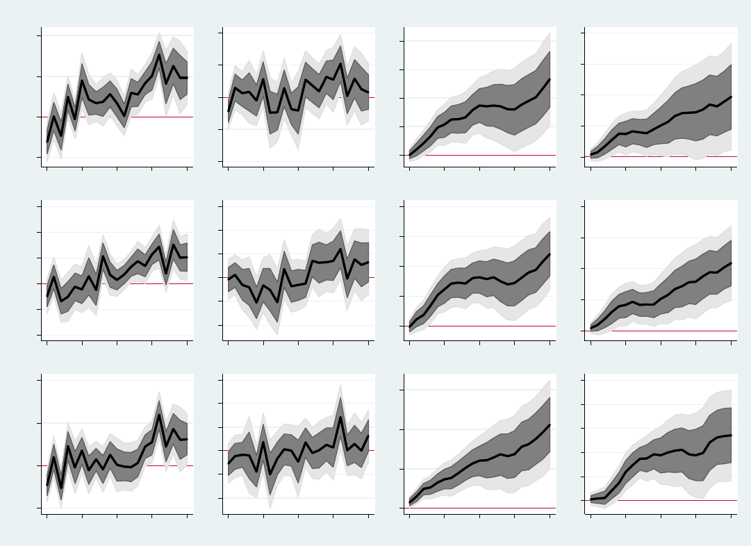
43
A
PPENDIX
F
IGURE
4:
R
OBUSTNESS OF
B
ASELINE
I
NEQUALITY
R
ESULTS TO
S
HORTER
MA
L
AGS
Note: The figure presents impulse responses of income inequality to 100 b.p. contractionary monetary policy shocks, using I=12 lags of monetary policy shocks.
The dark and light grey shaded areas indicate one and 1.65 standard deviation confidence intervals respectively. Time (horizontal axis) is in quarters. “P-val” are
for the null hypothesis that the impulse response is zero for every quarter plotted. See section 3.3 for details.
-.02 0 .02 .04
st.dev.
0 5 10 15 20
Income (p-val = 0.000)
-.04 -.02 0 .02 .04
st.dev.
0 5 10 15 20
Earnings (p-val = 0.023)
0 .02 .04 .06 .08
st.dev.
0 5 10 15 20
Expenditure (p-val = 0.003)
0 .02 .04 .06 .08
st.dev.
0 5 10 15 20
Consumption (p-val = 0.064)
-.01 -.005 0 .005 .01 .015
Gini
0 5 10 15 20
Income (p-val = 0.001)
-.01 -.005 0 .005 .01 .015
Gini
0 5 10 15 20
Earnings (p-val = 0.000)
0 .01 .02 .03 .04
Gini
0 5 10 15 20
Expenditure (p-val = 0.000)
0 .01 .02 .03 .04
Gini
0 5 10 15 20
Consumption (p-val = 0.002)
-.05 0 .05 .1
90-10
0 5 10 15 20
Income (p-val = 0.000)
-.1 -.05 0 .05 .1 .15
90-10
0 5 10 15 20
Earnings (p-val = 0.015)
0 .1 .2 .3
90-10
0 5 10 15 20
Expenditure (p-val = 0.002)
0 .05 .1 .15 .2 .25
90-10
0 5 10 15 20
Consumption (p-val = 0.000)

44
A
PPENDIX
F
IGURE
5:
R
OBUSTNESS OF
B
ASELINE
I
NEQUALITY
R
ESULTS TO
L
ONGER
AR
L
AGS
Note: The figure presents impulse responses of income inequality to 100 b.p. contractionary monetary policy shocks, using J=4 lags of dependent variable. The
dark and light grey shaded areas indicate one and 1.65 standard deviation confidence intervals respectively. Time (horizontal axis) is in quarters. “P-val” are for
the null hypothesis that the impulse response is zero for every quarter plotted. See section 3.3 for details.
-.02 0 .02 .04 .06
st.dev.
0 5 10 15 20
Income (p-val = 0.001)
-.04 -.02 0 .02 .04
st.dev.
0 5 10 15 20
Earnings (p-val = 0.001)
0 .02 .04 .06 .08
st.dev.
0 5 10 15 20
Expenditure (p-val = 0.014)
-.02 -.01 0 .01 .02 .03
st.dev.
0 5 10 15 20
Consumption (p-val = 0.576)
-.01 -.005 0 .005 .01 .015
Gini
0 5 10 15 20
Income (p-val = 0.004)
-.02 -.01 0 .01
Gini
0 5 10 15 20
Earnings (p-val = 0.000)
0 .01 .02 .03 .04
Gini
0 5 10 15 20
Expenditure (p-val = 0.001)
-.01 0 .01 .02 .03
Gini
0 5 10 15 20
Consumption (p-val = 0.004)
-.05 0 .05 .1
90-10
0 5 10 15 20
Income (p-val = 0.000)
-.15 -.1 -.05 0 .05 .1
90-10
0 5 10 15 20
Earnings (p-val = 0.023)
0 .1 .2 .3
90-10
0 5 10 15 20
Expenditure (p-val = 0.067)
-.05 0 .05 .1 .15
90-10
0 5 10 15 20
Consumption (p-val = 0.000)

45
A
PPENDIX
F
IGURE
6:
R
OBUSTNESS OF
B
ASELINE
I
NEQUALITY
R
ESULTS TO
D
ROPPING THE
V
OLCKER
D
ISINFLATION
Note: The figure presents impulse responses of income inequality to 100 b.p. contractionary monetary policy shocks, starting the time period in 1985Q1. The
dark and light grey shaded areas indicate one and 1.65 standard deviation confidence intervals respectively. Time (horizontal axis) is in quarters. “P-val” are for
the null hypothesis that the impulse response is zero for every quarter plotted. See section 3.3 for details.
-.02 0 .02 .04 .06
st.dev.
0 5 10 15 20
Income (p-val = 0.000)
-.05 0 .05
st.dev.
0 5 10 15 20
Earnings (p-val = 0.009)
0 .05 .1
st.dev.
0 5 10 15 20
Expenditure (p-val = 0.000)
-.02 0 .02 .04
st.dev.
0 5 10 15 20
Consumption (p-val = 0.001)
-.01 0 .01 .02
Gini
0 5 10 15 20
Income (p-val = 0.000)
-.02 -.01 0 .01
Gini
0 5 10 15 20
Earnings (p-val = 0.000)
0 .01 .02 .03 .04
Gini
0 5 10 15 20
Expenditure (p-val = 0.000)
-.01 0 .01 .02 .03
Gini
0 5 10 15 20
Consumption (p-val = 0.001)
-.05 0 .05 .1 .15
90-10
0 5 10 15 20
Income (p-val = 0.001)
-.2 -.1 0 .1 .2
90-10
0 5 10 15 20
Earnings (p-val = 0.004)
0 .1 .2 .3 .4
90-10
0 5 10 15 20
Expenditure (p-val = 0.007)
-.05 0 .05 .1 .15 .2
90-10
0 5 10 15 20
Consumption (p-val = 0.000)

46
A
PPENDIX
F
IGURE
7:
R
OBUSTNESS OF
B
ASELINE
I
NEQUALITY
R
ESULTS TO
D
ROPPING
A
LL
R
ECESSIONS
Note: The figure presents impulse responses of income inequality to 100 b.p. contractionary monetary policy shocks, dropping all recession periods. The dark
and light grey shaded areas indicate one and 1.65 standard deviation confidence intervals respectively. Time (horizontal axis) is in quarters. “P-val” are for the
null hypothesis that the impulse response is zero for every quarter plotted. See section 3.3 for details.
-.02 0 .02 .04 .06
st.dev.
0 5 10 15 20
Income (p-val = 0.000)
-.04 -.02 0 .02 .04 .06
st.dev.
0 5 10 15 20
Earnings (p-val = 0.001)
0 .05 .1
st.dev.
0 5 10 15 20
Expenditure (p-val = 0.022)
0 .02 .04 .06 .08
st.dev.
0 5 10 15 20
Consumption (p-val = 0.005)
-.005 0 .005 .01 .015 .02
Gini
0 5 10 15 20
Income (p-val = 0.000)
-.01 -.005 0 .005 .01 .015
Gini
0 5 10 15 20
Earnings (p-val = 0.000)
0 .01 .02 .03 .04
Gini
0 5 10 15 20
Expenditure (p-val = 0.000)
0 .01 .02 .03
Gini
0 5 10 15 20
Consumption (p-val = 0.000)
-.05 0 .05 .1
90-10
0 5 10 15 20
Income (p-val = 0.000)
-.1 0 .1 .2
90-10
0 5 10 15 20
Earnings (p-val = 0.004)
0 .1 .2 .3 .4
90-10
0 5 10 15 20
Expenditure (p-val = 0.000)
0 .05 .1 .15 .2
90-10
0 5 10 15 20
Consumption (p-val = 0.000)
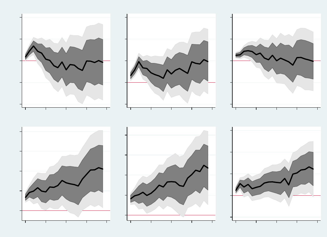
47
A
PPENDIX
F
IGURE
8:
R
OBUSTNESS OF
C
ONSUMPTION AND
E
XPENDITURE
I
NEQUALITY
R
ESULTS TO
A
LTERNATIVE
T
IMING
A
SSUMPTIONS
Note: The figure presents impulse responses of consumption and expenditure inequality to 100 b.p. contractionary monetary policy shocks, when analysis is done
across cohorts as described in section 3.2 and Appendix A. The dark and light grey shaded areas indicate one and 1.65 standard deviation confidence intervals
respectively. Time (horizontal axis) is in quarters. “P-val” are for the null hypothesis that the impulse response is zero for every quarter plotted. See section 3.3
for details.
-.02 -.01 0 .01 .02
st.dev.
0 5 10 15 20
Consumption (p-val = 0.000)
-.005 0 .005 .01 .015
Gini
0 5 10 15 20
Consumption (p-val = 0.000)
-.1 -.05 0 .05 .1
P90-P10
0 5 10 15 20
Consumption (p-val = 0.000)
0 .01 .02 .03 .04
st.dev.
0 5 10 15 20
Expenditures (p-val = 0.000)
0 .005 .01 .015 .02
Gini
0 5 10 15 20
Expenditures (p-val = 0.000)
-.05 0 .05 .1 .15
P90-P10
0 5 10 15 20
Expenditure (p-val = 0.000)

48
A
PPENDIX
F
IGURE
9:
R
OBUSTNESS OF
B
ASELINE
I
NEQUALITY
R
ESULTS TO
C
ONTROLLING FOR
H
OUSEHOLD
O
BSERVABLE
C
HARACTERISTICS
Notes: The figure plots impulse responses of inequality measures (cross-sectional standard deviations) for total income (first column), salary income (second
column), total expenditures (third column), and consumption (fourth column) in response to a 1 percentage point (100 b.p.) contractionary monetary policy
shock. The dark and light grey shaded areas indicate one and 1.65 standard deviation confidence intervals respectively. “P-val” are for the null hypothesis that the
impulse response is zero for every quarter plotted. Time (horizontal axis) is in quarters. Row 1 includes benchmark measures of inequality, row 2 adjusts for
household size (OECD equivalence scale), and row 3 controls for household observables. See section 3.3 for details.
-.02 0 .02 .04
baseline
0 5 10 15 20
Income (p-val = 0.000)
-.04 -.02 0 .02 .04
baseline
0 5 10 15 20
Earnings (p-val = 0.008)
0 .02 .04 .06 .08 .1
baseline
0 5 10 15 20
Expenditure (p-val = 0.002)
0 .02 .04 .06
baseline
0 5 10 15 20
Consumption (p-val = 0.006)
-.02 0 .02 .04
control for HH size
0 5 10 15 20
Income (p-val = 0.001)
-.04 -.02 0 .02 .04
control for HH size
0 5 10 15 20
Earnings (p-val = 0.007)
-.02 0 .02 .04 .06
control for HH size
0 5 10 15 20
Expenditure (p-val = 0.000)
-.02 -.01 0 .01 .02 .03
control for HH size
0 5 10 15 20
Consumption (p-val = 0.007)
-.02 0 .02 .04
control for HH observables
0 5 10 15 20
Income (p-val = 0.004)
-.04 -.02 0 .02 .04
control for HH observables
0 5 10 15 20
Earnings (p-val = 0.004)
-.02 0 .02 .04 .06
control for HH observables
0 5 10 15 20
Expenditure (p-val = 0.000)
-.02 -.01 0 .01 .02 .03
control for HH observables
0 5 10 15 20
Consumption (p-val = 0.000)

49
A
PPENDIX
F
IGURE
10:
L
EVEL AND
S
HOCKS TO THE
F
EDERAL
R
ESERVE
’
S
T
ARGET
R
ATE OF
I
NFLATION
Panel A. Target Rate
Panel B. Shocks to the Target Rate
Notes: The figure plots two measures of shocks to the inflation target rate of the U.S. Federal Reserve as estimated by
Ireland (2006) and Coibion and Gorodnichenko (2011). Grey shaded areas are U.S. recessions. See section 5 for details.
0 1 2 3 4 5 6 7 8 9 10
Percent
1970 1975 1980 1985 1990 1995 2000 2005 2010
Coibion and Gorodnichenko (2011)
Ireland (2006)
-3 -2 -1 0 1
Percent
1980 1985 1990 1995 2000 2005 2010
Coibion and Gorodnichenko (2011)
Ireland (2006)

50
A
PPENDIX
F
IGURE
11:
D
ISTRIBUTIONAL
E
FFECTS OF
S
HOCKS TO THE
F
ED
’
S
I
NFLATION
T
ARGET
Notes: The figure plots the responses of the differences between the 90
th
and 50
th
percentiles (blue solid line) as well as the difference between the 10
th
and 50
th
percentiles (red solid line) of income, earnings, expenditure and consumption distributions of households in the CEX to a 1 percentage point (100 b.p.) decrease
in the Fed’s inflation target. Dashed lines show the 66% (one standard deviation) confidence intervals. Time (horizontal axis) is in quarters. “P-val” are for the
null hypothesis that the difference between the two impulse responses in each figure is zero for every quarter plotted. See section 5 for details.
-.06 -.04 -.02 0 .02 .04
0 5 10 15 20
Income (p-val = 0.000)
-.15 -.1 -.05 0 .05
0 5 10 15 20
P10-P50 P90-P50
CI 66% CI 66%
Earnings (p-val = 0.000)
-.2 -.1 0 .1
0 5 10 15 20
Expenditure (p-val = 0.000)
-.15 -.1 -.05 0 .05 .1
0 5 10 15 20
Consumption (p-val = 0.000)

51
A
PPENDIX
F
IGURE
12:
D
ISTRIBUTIONAL
E
FFECTS OF
S
HOCKS IDENTIFIED FROM
F
ED
F
UNDS
F
UTURES
.
Notes: the top panel shows responses of standard deviation of measures of income and consumption to monetary policy shocks identified from changes in fed
funds futures around FOMC announcements. This series of monetary policy shocks is taken from Gorodnichenko and Weber (2016). The bottom panel shows
responses of standard deviation of measures of income and consumption to monetary policy shocks identified as in Romer and Romer (2004). For all panels, the
estimation sample is 1994Q1-2008Q4. Time (horizontal axis) is in quarters. The figure plots one and 1.65 standard deviation confidence intervals as dark and
light grey shaded areas respectively. “p-val” are for the null hypothesis that the impulse response is zero for every quarter plotted.
-.05 0 .05 .1 .15
st.dev.
0 5 10 15 20
Income (p-val = 0.000)
FFF shocks (GW)
-.1 -.05 0 .05 .1
st.dev.
0 5 10 15 20
Earnings (p-val = 0.000)
FFF shocks (GW)
-.05 0 .05 .1 .15
st.dev.
0 5 10 15 20
Expenditure (p-val = 0.000)
FFF shocks (GW)
-.05 0 .05 .1
st.dev.
0 5 10 15 20
Consumption (p-val = 0.000)
FFF shocks (GW)
-.04 -.02 0 .02 .04 .06
st.dev.
0 5 10 15 20
Income (p-val = 0.000)
Romer-Romer shocks
-.05 0 .05
st.dev.
0 5 10 15 20
Earnings (p-val = 0.000)
Romer-Romer shocks
-.02 0 .02 .04 .06 .08
st.dev.
0 5 10 15 20
Expenditure (p-val = 0.000)
Romer-Romer shocks
-.01 0 .01 .02 .03 .04
st.dev.
0 5 10 15 20
Consumption (p-val = 0.000)
Romer-Romer shocks

52
A
PPENDIX
F
IGURE
13:
R
ESPONSE OF
CEX
AND
NIPA
CONSUMPTION TO A CONTRACTIONARY MONETARY POLICY SHOCK
.
Notes: the figure plots impulse response of CEX consumption (see the text for the definition; solid blue line) and NIPA’s private spending on non-durables
(solid, red line) to one percentage point contractionary monetary policy shock identified as in Romer and Romer (2004). The estimation sample is 1980Q1-
2008Q4. Time (horizontal axis) is in quarters. The figure plots one standard deviation confidence intervals (66% coverage) as dashed lines. See section 3.1 for
details.
-.04 -.02 0 .02
0 5 10 15 20
CEX NIPA
66% CI 66% CI
Consumption

53
A
PPENDIX
T
ABLE
1:
C
ORRELATIONS AND
V
OLATILITIES OF
I
NEQUALITY
M
EASURES
Panel A: Correlations across Inequality Measures
Corr(SD,Gini)
Corr(SD,90
th
-
10
th
)
Corr(Gini,90
th
-
10
th
)
Income Inequality
0.90
0.93
0.89
Earnings Inequality
0.64
0.88
0.60
Expenditures Inequality
0.88
0.89
0.75
Consumption Inequality
0.62
0.79
0.43
Panel B: Correlations of Inequality in Income, Salary, Expenditures and Consumption
SD
Gini
90
th
-
10
th
Corr(Income, Earnings)
0.25
0.53
0.19
Corr(Income, Expenditures)
0.32
0.55
0.22
Corr(Income, Consumption)
0.13
0.66
0.04
Corr(Earnings, Expenditures)
0.23
0.47
0.17
Corr(Earnings, Consumption)
-
0.08
0.32
-
0.04
Corr(Expenditures, Consumption)
0.57
0.79
0.39
Panel C: Volatility of Inequality Measures
SD
Gini
90
th
-
10
th
Income Inequality
0.049
0.017
0.096
Earning Inequality
0.032
0.012
0.108
Expenditures Inequality
0.016
0.011
0.050
Consumption Inequality
0.009
0.008
0.034
Notes: Panel A presents correlation coefficients of inequality in income, earnings, expenditures, and consumption across
the different measures of each: SD denotes cross-sectional standard deviation, Gini denotes Gini coefficients, and 90
th
-10
th
denotes the log difference between the 90
th
and 10
th
percentiles of the cross-sectional distribution. Panel B presents
correlation coefficients between each pair of income, earnings, expenditures, and consumption inequality for each
approach (SD, Gini or 90
th
-10
th
) to measuring inequality. Panel C presents standard deviations of each measure of
inequality. All data is from 1980Q1 to 2008Q4.

54
A
PPENDIX
T
ABLE
2:
D
ECOMPOSITION OF
I
NCOME BY
Q
UINTILE
Quintiles by
consumption of
nondurables and
services
Share of income source
Ratio of mean
consumption of
nondurables and services to
mean consumption of
nondurables and services in the
3
rd
quintile
Labor
Earnings
Business Financial Other
(1) (2) (3) (4)
(5)
Panel A: 1980s
1 0.352 0.022 0.112 0.515 0.42
2 0.588 0.040 0.112 0.260 0.73
3 0.694 0.057 0.096 0.153 1.00
4 0.762 0.059 0.081 0.098 1.34
5 0.767 0.088 0.078 0.067 2.18
Panel B: 1990s
1 0.380 0.020 0.106 0.494 0.43
2 0.597 0.040 0.097 0.267 0.73
3 0.704 0.050 0.086 0.160 1.00
4 0.770 0.056 0.071 0.103 1.35
5 0.773 0.082 0.076 0.069 2.27
Panel C: 2000s
1 0.435 0.019 0.086 0.460 0.43
2 0.653 0.029 0.085 0.234 0.73
3 0.740 0.037 0.072 0.151 1.00
4 0.801 0.042 0.065 0.092 1.36
5 0.812 0.051 0.071 0.065 2.32
Notes: The table presents a decomposition of sources of household income in the CEX by quintile. Households are sorted into quintiles using their consumption
levels of nondurables and services. Income categories include labor earnings, business income, financial income, and other sources of income. See section 3.4 in
the text for details.

55
A
PPENDIX
T
ABLE
3:
D
ECOMPOSITION OF
E
XPENDITURES AND
C
ONSUMPTION BY
Q
UINTILE
Quintiles by
consumption of
nondurables
and services
Shares in consumption
Selected shares in total spending
Ratio of
total
spending to
consumption
of nondurables
and services
Nondurables Durables Services
Interest
sensitive
expenditures
Mortgage
payments
Purchases of
new vehicles
(1) (2) (3)
(4) (5) (6)
(7)
Panel A: 1980s
1
0.696 0.053 0.251
0.105 0.017 0.015 1.87
2
0.682 0.080 0.238
0.163 0.041 0.032 1.86
3
0.666 0.097 0.238
0.197 0.062 0.039 1.84
4
0.653 0.104 0.243
0.232 0.081 0.045 1.83
5
0.612 0.111 0.277
0.253 0.084 0.054 1.80
Panel B: 1990s
1
0.654 0.056 0.289
0.113 0.023 0.016 2.13
2
0.641 0.077 0.282
0.169 0.053 0.032 2.05
3
0.632 0.094 0.274
0.213 0.076 0.040 2.03
4
0.616 0.107 0.277
0.246 0.095 0.045 2.01
5
0.569 0.115 0.316
0.268 0.100 0.052 1.92
Panel C: 2000s
1
0.634 0.053 0.313
0.121 0.036 0.014 2.24
2
0.623 0.067 0.309
0.181 0.073 0.029 2.12
3
0.619 0.081 0.300
0.216 0.094 0.035 2.09
4
0.602 0.094 0.304
0.254 0.108 0.044 2.08
5
0.543 0.106 0.351
0.278 0.108 0.052 1.99
Note: The table presents a decomposition of consumption and expenditures in the CEX by quintile. Households are sorted into quintiles using their consumption
levels of nondurables and services. Consumption includes nondurables, services and durables. Total spending is the sum of consumption and other expenditures,
including auto purchases, mortgage payments among others. Interest sensitive spending includes expenditure on new vehicles, furniture and durable housing
items, education, durable entertainment, mortgage payments, and mortgage down-payments. See section 3.3 in the text for details.
56
Appendix A: Cohort Analysis
Consider consumption data collected in the CEX over May 2015 – July 2015. For each survey month we
define a cohort: May 2015 (cohort B), June 2015 (cohort C), and July 2015 (cohort A). Cohort A’s survey
response covers the months of April, May and June. Cohort B’s survey response covers the months of
February, March, and April. Cohort C’s survey response covers the months of March, April and May.
Thus, cohort A’s reporting period coincides with the calendar quarter. Cohort B’s reporting period is such
that, apart from consumption in the second quarter, the CEX measure of consumption includes 1/3 of
consumption from 2015Q2 and 2/3 of consumption from 2015Q1. When households in cohort B are
surveyed again in Aug 2015, their reported consumption covers 2/3 of consumption from 2015Q2 and ½
of consumption from 2015Q3. In similar spirit, the CEX measure of consumption for Cohort C includes
1/3 of consumption from 2015Q1 and 2/3 of consumption from 2015Q2. When surveyed next time in
September 2015, cohort C reports consumption which covers 1/3 of consumption from 2015Q2 and 2/3 of
consumption from 2015Q3. As we discussed in the text, BLS splits three-monthly consumption equally
across months during this period. The standard practice is to aggregate monthly consumption to quarterly
consumption. However, the timing of measurements means that calendar quarterly consumption has a
lagging component and a leading component.
This timing can introduce a complex serial correlation structure such that using standard VARs
may be problematic: one needs to introduce moving average (MA) terms or use many lags to proxy for
the MA terms. However, one can largely circumvent this problem by using direct projections a la Jorda
(2005) with a large number of shocks as control variables to allow for flexible shapes of the estimated
impulse response functions. As a result, our estimated impulse response functions should be interpreted as
estimates of responses averaged across different (monthly) horizons. In other words, the estimated
impulse response is a smoothed version of the true impulse response.
To see this intuition more formally, consider the following moving average representation for
consumption:
?
#
E
F
E
#E++
--.-
#
(1)
where ?
#
is a measure of inequality at time V,
#++
is the Romer-Romer shock, and --.-
#
is the residual.
Note that
#++
is unanticipated and serially uncorrelated by construction. Shock
#E++
is orthogonal to
--.-
#
by construction as well. Now suppose that we observe a measure of inequality that is a two-sided
moving average of ?
#
. This case corresponds to the time aggregation in the CEX when for a given
calendar quarter we use consumption from adjacent quarters. Specifically, we assume that ?W
#
X
C
?
#$C
C
. It follows that
?W
#
X
C
?
#$C
C
X
C
(
E
F
E
#E$C++
--.-
#$C
)
C
X
#$++
X
X
#++
X
X
X
#++
X
Y
X
X
#++
X
Z
X
Y
X
#Y++
[
X
F
X
F
X
F
#F$++
X
F
X
F
#F++
X
F
#F++
X
C
--.-
#$C
\
]
E
F$
E
#E++
--.-^
#
(2)
where ]
X
, ]
X
X
, ]
X
X
X
, ]
X
Y
X
X
,
…, ]
F
X
F
X
F
X
F
, ]
F
X
F
X
F
, ]
F$
X
F
.
Note that given the properties of shock series
#++
, we still have that
#E++
is orthogonal to
--.-^
#
and thus we can estimate specification (2) by OLS. Also note that, while using a moving average

57
measure of inequality ?W
#
introduces a lead of
#,++
, this additional term does not have a material effect in
practice. First, users of the Romer-Romer shocks typically impose the restriction that monetary shocks do
not have a contemporaneous effect on the real side of the economy, that is,
0, and hence ]
0.
Second, even if
_ 0, the shocks
#,+ +
are not serially correlated and therefore excluding leads of
shocks from specification (2) does not affect estimates of coefficients on the current and lagged values of
shocks. In summary, the impulse response function
`
]
E
a
E
F$
estimated using specification (2) (this
moving average representation corresponds to the direct projection approach of Jorda (2005)) recovers a
smoothed version of the impulse response for the corresponding series that is not aggregated across time.
To further explore the importance of the timing for our results, one can change the aggregation of the
Romer-Romer shocks to match the reporting frequency for each cohort in the CEX. Appendix Tables A1-
A3 show the timing of reported consumption and the Romer-Romer shock series with the corresponding
timing. Note that the time period corresponds to the calendar quarter only for Cohort A, while for other
cohorts it is shifted by one month and two months relative to the calendar time.
Appendix Table A1. Romer-Romer shocks and measured consumption for cohort A.
Period
Romer-Romer shock,
#
,
++
A
CEX Consumption
1
(
Z
,
*bL
Z
,
cde
Z
,
fbg
)
h
Z
,
Aigj
A
2
(
Z
,
Aig
Z
,
fbP
Z
,
*kL
)
h
Z
,
*kjP
A
3
(
Z
,
*kj
Z
,
AkO
Z
,
Fdi
)
h
Z
,
lm#
A
4
(
Z
,
lm#
Z
,
nop
Z
,
qdm
)
h
r
,
*bL
A
5
(
r
,
*bL
r
,
cde
r
,
fbg
)
h
r
,
Aig
A
6
(
r
,
Aig
r
,
fbP
r
,
*kL
)
h
r
,
*kj
A
7
(
r
,
*kj
r
,
AkO
r
,
Fdi
)
h
r
,
lm#
A
8
(
r
,
lm#
r
,
nop
r
,
qdm
)
h
s
,
*bL
A
9
(
s
,
*bL
s
,
cde
s
,
fbg
)
h
s
,
Aig
A
10
(
s
,
Aig
s
,
fbP
s
,
*kL
)
h
s
,
*kj
A
11
(
s
,
*kj
s
,
AkO
s
,
Fdi
)
h
s
,
lm#
A
12
(
s
,
lm#
s
,
nop
s
,
qdm
)
h
t
,
*bL
A
Appendix Table A2. Romer-Romer shocks and measured consumption for cohort B.
Period
Romer-Romer shock,
#
,
++
G
CEX Consumption
1
(
Z
,
cde
Z
,
fbg
Z
,
Aig
)
h
Z
,
fbP
G
2
(
Z
,
fbP
Z
,
*kL
Z
,
*kj
)
h
Z
,
AkO
G
3
(
Z
,
AkO
Z
,
Fdi
Z
,
lm#
)
h
Z
,
nop
G
4
(
Z
,
nop
Z
,
qdm
r
,
*bL
)
h
r
,
cde
G
5
(
r
,
cde
r
,
fbg
r
,
Aig
)
h
r
,
fbP
G
6
(
r
,
fbP
r
,
*kL
r
,
*kj
)
h
r
,
AkO
G
7
(
r
,
AkO
r
,
Fdi
r
,
lm#
)
h
r
,
nop
G
8
(
r
,
nop
r
,
qdm
s
,
*bL
)
h
s
,
cde
G
9
(
s
,
cde
s
,
fbg
s
,
Aig
)
h
s
,
fbP
G
10
(
s
,
fbP
s
,
*kL
s
,
*kj
)
h
s
,
AkO
G
11
(
s
,
AkO
s
,
Fdi
s
,
lm#
)
h
s
,
nop
G
12
(
s
,
nop
s
,
qdm
t
,
*bL
)
h
t
,
cde
G

58
Appendix Table A 3. Romer-Romer shocks and measured consumption for cohort C.
Period
Romer-Romer shock,
#
,
++
H
CEX Consumption
1
(
Z
,
fbg
Z
,
Aig
Z
,
fbP
)
h
Z
,
*kL
H
2
(
Z
,
*kL
Z
,
*kj
Z
,
AkO
)
h
Z
,
Fdi
H
3
(
Z
,
Fdi
Z
,
lm#
Z
,
nop
)
h
Z
,
qdm
H
4
(
Z
,
qdm
r
,
*bL
r
,
cde
)
h
r
,
fbg
H
5
(
r
,
fbg
r
,
Aig
r
,
fbP
)
h
r
,
*kL
H
6
(
r
,
*kL
r
,
*kj
r
,
AkO
)
h
r
,
Fdi
H
7
(
r
,
Fdi
r
,
lm#
r
,
nop
)
h
r
,
qdm
H
8
(
r
,
qdm
s
,
*bL
s
,
cde
)
h
s
,
fbg
H
9
(
s
,
fbg
s
,
Aig
s
,
fbP
)
h
s
,
*kL
H
10
(
s
,
*kL
s
,
*kj
s
,
AkO
)
h
s
,
Fdi
H
11
(
s
,
Fdi
s
,
lm#
s
,
nop
)
h
s
,
qdm
H
12
(
s
,
qdm
t
,
*bL
t
,
cde
)
h
t
,
fbg
H
Once the timing of shocks is aligned for each cohort, we can estimate the impulse response of inequality
to monetary shocks as a system of equations:
Δ?
#$%
(@
A
)
B
C
%
D
C
Δ?
#C
(@
A
)
B
E
%
F
E
#E,++
A
--.-
#,%
A
,/ 0,…,2
Δ?
#$%
(@
G
)
B
C
%
D
C
Δ?
#C
(@
G
)
B
E
%
F
E
#E,++
G
--.-
#,%
G
,/ 0,…,2
Δ?
#$%
(@
H
)
B
C
%
D
C
Δ?
#C
(@
H
)
B
E
%
F
E
#E,++
H
--.-
#,%
H
,/ 0,…,2
where each equation corresponds to a cohort, / indexes horizon in the direct projection, ?
#
(@
u
) is a
measure of inequality for time V and cohort v,
#,++
u
is the value of the Romer-Romer shock at time V
calculated for cohort v. The impulse response is calculated as cumulative sum of
8
5
%
9
%
7
. Note that
the slopes
8
C
%
9
and
8
E
%
9
are the same across cohorts (equations). This restriction is aimed to increase
the precision of estimates.
Also note that the correct inference must take into account the serial and cross-sectional correlation of the
error terms. This issue is addressed by using Driscoll and Kraay (1998) standard errors that allow for
arbitrary serial and cross-sectional correlation of errors.
The downside of this approach is that we use only a third of the sample to compute a measure of
inequality for a given quarter. As a result, inequality measures calculated for each cohort separately are
noisier than the corresponding inequality measured calculated for the whole sample.

59
Appendix B: CEX Data Appendix
This section describes the construction of the Consumer Expenditure data in more detail. For years 1980
to 2005 we compile the data directly from the raw ASCII files available from the Inter-university
Consortium for Political and Social Research (ICPSR). From year 2006 on we use the public-use
microdata provided by the Bureau of Labor Statistics (BLS). All expenditure data is aggregated up from
the disaggregated MTAB files (adding ITAB files where necessary; e.g., occupational expenses before
2001Q1), and income data is derived from the FMLY files. Additional information from the MEMB files
is used in the tax imputation procedure outlined below, such as the number of qualifying dependents, etc.
As recommended by the BLS, we sum expenditures that occur in the same month but are reported
in different interviews. We then drop the fourth and higher observation for household-interviews with
more than three monthly observations. These latter observations appear to be outliers relative to the
reported expenditures for the first three months. We also drop households that report zero expenditure on
food in any interview (adding both food at home and food away from home). Finally, we drop the few
households that report negative expenditures for categories that cannot be negative according to the data
codebook, such as expenditures for elderly care.
We correct sample breaks due to slight changes in the questionnaire of the following variables:
food at home (1982Q1-88Q1), food away from home (2007Q2), personal care services (2001Q2),
occupation expenditures (2001Q2), and property taxes (1991Q1). In particular, we regress each
expenditure series on a time trend and indicators for the corresponding sample breaks. For instance, we
regress expenditures on food at home on a time trend and a dummy for the period 1982Q1-87Q4. We then
subtract from the original series the effect of the dummies.
The BLS began imputing income in 2004 but did not impute previous years. Furthermore, non-
imputed income values are not available for years 2004 and 2005. We therefore follow Fisher, Johnson
and Smeeding (2013) and replicate the BLS methodology as closely as possible to impute all income
prior to 2004. For respondents who refused to provide an exact dollar amount but instead provided an
answer from a bracketed range, we use the mid-point of the bracket. We then impute the remaining
missing income observations (i.e. "invalid blanks") using annual regressions of income on age and age
squared of the reference person, fixed effects for the income reporting date, and a fully saturated model of
the following categorical variables: the reference person's gender, race, education, number of weeks
worked full or part time in the last 12 month; unadjusted family size; the number of children less than 18;
the number of persons over 64; and the number of earners. All regressions use sampling weights. To
account for the sampling uncertainty, we add residuals drawn randomly with replacement from the
sampling distribution to the predicted values. We then trim values above the top-coding threshold at the
top coding value.
Finally, since self-reported taxes are of low quality, we follow the recommendation of the BLS
and impute tax liabilities based on the higher quality income data and household demographics. In
particular, we impute taxes for each household in the survey using the NBER TAXSIM calculator. We
use an iterative procedure determining the itemization status of each household in a first step in order to
account for deductions that depend on the household's adjusted gross income (AGI); for example health
care or job expenses. We then use the household's inferred AGI together with its filing status and
demographics to impute its final tax liabilities. The code is available at www.nber.org/~taxsim/to-
taxsim/cex-kueng/cex.do.
60
We aggregate spending to the (calendar) quarterly frequency from the monthly frequency. While
the resulting measures introduces a moving average structure, the resulting series maximizes the sample
used for calculating inequality. As we discuss in Appendix A, results are similar when we use three-
monthly frequency that does not coincide with calendar quarters for some households.
When we compute inequality measures, we censor each spending and income series at the
corresponding values of the top and bottom percentiles. Note that for aggregated spending/income series,
we first aggregate and then apply censoring.
To calculate residual inequality, we control for: 1) quartic age polynomial; 2) six educational
attainment dummy variables; 3) a set of dummy variables for each household size; 4) a set of dummy
variables for each number of children; 5) a set of dummy variables for race; 6) a set of dummy variables
for the number of earners. In additional checks, we also control for the number of interview (a proxy for
how complete a survey is) and/or exclude observations with incomplete income responses.
To adjust for differences in household size, we also use the OECD scale. Specifically, the
(effective) number of household members is calculated as follows: (head of household) + 0.7*(number of
adults [18 years old or older] – 1) + 0.5*(number of children).
Because the composition of households changes over time, we calculate changes in equality on
the sample on households present in both periods. For example, when we calculate the change in Gini
inequality from say 2001Q1 to 2001Q2, we do it only for households that are present in 2001Q1 and
2001Q2.
We use X-12 to seasonally adjust all inequality and transition probability series.
