
Graph Algorithms
Mirek Riedewald
This work is licensed under the Creative Commons Attribution 4.0 International License.
To view a copy of this license, visit http://creativecommons.org/licenses/by/4.0/.

Key Learning Goals
• Write the pseudo-code for breadth-first search
(BFS) in MapReduce and in Spark.
• Write the pseudo-code for single-source shortest
path in MapReduce and in Spark.
• Write the pseudo-code for PageRank (without
dangling pages) in MapReduce and in Spark.
• How can the single-source shortest path
algorithm detect that no more iterations are
needed?
• How can the PageRank algorithm detect that no
more iterations are needed?
2

Key Learning Goals
• Why is Spark better suited for BFS and BFS-
based algorithms than MapReduce?
• How can we handle dangling pages in
PageRank?
3

Introduction
• Graphs are very general and a
large variety of real-world
problems can be modeled
naturally as graph analysis or
mining problems. Data
occurring as graphs include:
– The hyperlink structure of the Web
– Social interactions, e.g., Facebook friendships, Twitter
followers, email flows, and phone call patterns
– Transportation networks, e.g., roads, bus routes, and
flights
– Relationships between genes, proteins, and diseases
• Since graphs are so general, many graph problems are
inherently complex—a perfect target for distributed
data-intensive computation.
4

Explanation for the Example
• This image shows a network of innovation
relationships in the state of Pennsylvania in
1990, collected by Christopher S. Dempwolf.
The node-link visualization is laid out with the Harel-
Koren FMS layout algorithm. Orange nodes are
companies, e.g., Westinghouse electric; silver nodes
inventors. Size indicates a measure of prominence.
Edge colors represent the type of a collaboration and
edges with similar routes are bundled together.
– Chaturvedi, S, Dunne, C, Ashktorab, Z, Zacharia, R, and
Shneiderman, B. “Group-in-a-Box meta-layouts for
topological clusters and attribute-based groups: space
efficient visualizations of network communities and their
ties”. In: CGF: Computer Graphics Forum 33.8 (2014), pp.
52-68
– Note: Cody Dunne is a faculty member in our college.
5
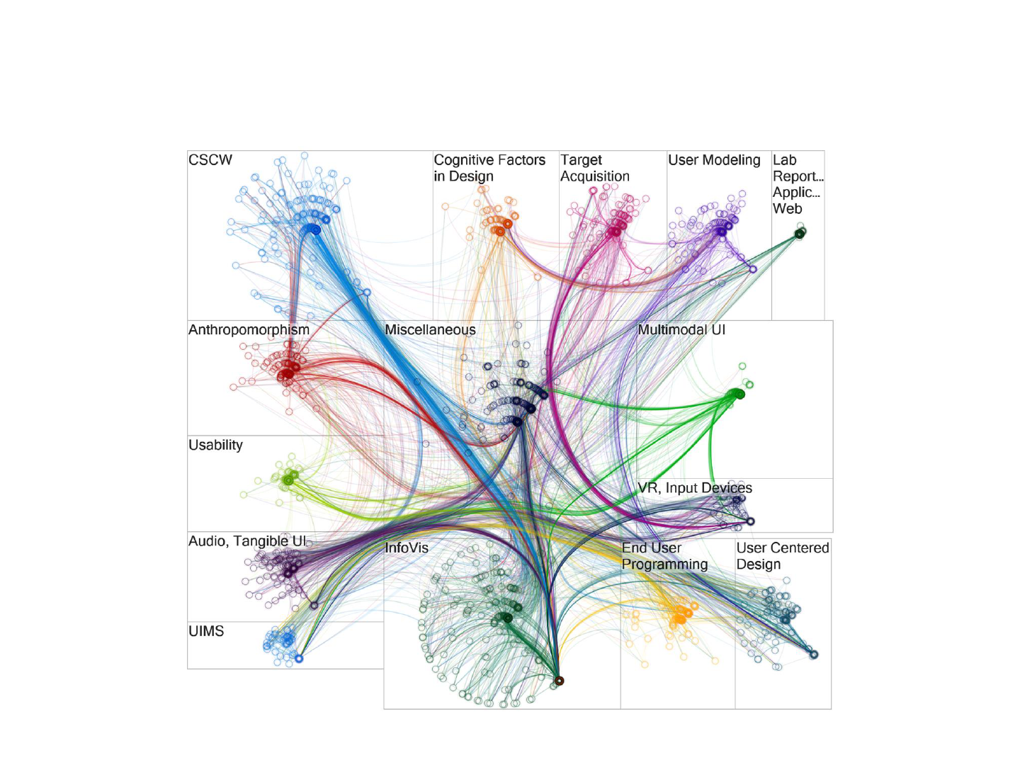
Relationships between CHI Topics
6

Explanation for the Example
• Papers of the ACM CHI conference,
grouped disjointly by the main topic
they cover and laid out individually for each topic
using a polar layout. Node colors show the
various groups, and the color of edges shows
citations from papers in that same colored group
to other papers. Edges with similar routes are
bundled together. Radius and angle encode the
number of citations and the betweenness
centrality (how much of a gatekeeper the paper is
between groups).
– Same reference as previous image.
7

What is a Graph?
• A graph consists of vertices (a.k.a. nodes) and edges (a.k.a. links)
between them. Vertex and edge labels can be used to encode
heterogeneous networks.
– In an online social network, a vertex could be a person annotated with
demographic information such as age. An edge could be annotated by
the type of relationship, e.g., “friend” or “family.” This richer structure
can improve the quality of the results obtained from graph analysis.
• We will focus on unlabeled graphs. Formally, a graph G is a pair (V,
E), where V is a set of vertices and E is set of edges, such that
.
• Edges can be directed or undirected. In a directed graph, edges (v1,
v2) and (v2, v1) are different, while in an undirected graph they are
the same. A standard trick is to encode undirected edge (v1, v2)
using the corresponding two directed edges.
– A road network should be modeled as a directed graph, because of the
existence of one-way streets.
• Graphs might contain cycles. If a graph does not contain any cycle, it
is acyclic.
8

Graph Problems
• There is a huge variety of graph analysis problems, including the following
common examples.
• Graph search and path planning
– Find driving directions from point A to point B.
– Recommend new friends in a social network.
– Find the best route for IP packets or delivery trucks.
• Graph clustering
– Identify user communities in social networks based on graph structure, e.g., connectedness.
– Partition a large graph into homogeneous partitions to parallelize graph processing.
• Minimum spanning trees
– Find the connected graph of minimum total edge weight.
• Bipartite graph matching
– Match nodes on the “left” with nodes on “right” side. For example, match job seekers and
employers, singles looking for dates, or papers with qualified reviewers.
• Maximum flow
– Determine the greatest possible traffic between a source and a sink node, e.g., to optimize
transportation networks.
• Finding “special” vertices
– Find vertices that are of importance, e.g., disease hubs, leaders of a community, authoritative
Web pages on a topic, or people with influence.
9

US Senate Co-Voting Patterns
10

Explanation for the Example
• US Senate co-voting patterns in 2007.
Nodes represent senators and are
colored by party: blue democrats, red republicans, purple
independents. Edges join pairs of senators that vote the
same way at least 70% of the time. The left image shows a
node-link visualization of the data arranged using the
Fruchterman Reingold network layout algorithm. The right
shows the same network after applying motif
simplification, which aggregates maximal cliques in the
network into tapered square glyphs. In this the size of
edges shows the overall number of edges between any pair
of glyphs or glyphs and nodes.
– Dunne, C and Shneiderman, B. “Motif simplification: improving
network visualization readability with fan, connector, and clique
glyphs”. In: CHI '13: Proc. SIGCHI Conference on Human Factors
in Computing Systems. 2013, pp. 3247-3256
11

Graph Representations
• Graphs are usually represented in one of these
three formats:
– Adjacency matrix
– Adjacency list
– Set of individual edges
• We will take a quick look at each of them.
12

Adjacency-Matrix Representation
• The adjacency matrix M represents a graph in a
matrix of size |V| by |V|. Its size is quadratic in
the number of vertices. Entry M(i,j) contains the
weight of the edge from vertex i to vertex j; or 0 if
there is no edge.
– The adjacency matrix of an undirected graph is
symmetric along the diagonal.
13
1 2 3
1 0 1 0
2 1 0 1
3 0 0 1
1
2
3

Adjacency Matrix Properties
• Pro: An adjacency matrix is easy to process using linear
algebra. For example, in product MM, entry (i,j) indicates
if there exists a two-step path from vertex i to vertex j (if
the value is non-zero) or not (if the value is zero).
• Pro: An operation on outgoing edges of a vertex (also called
“outlinks”) corresponds to an iteration over a row of the
adjacency matrix. An operation on incoming edges of a
vertex (also called “inlinks”) corresponds to an iteration
over a column.
• Con: For large graphs, the adjacency matrix tends to be
very sparse as most vertex pairs are not connected by an
edge. For those graphs this representation is inefficient (in
terms of storage cost) or even infeasible. Consider the
Facebook friendship graph: for 1 billion users, even if every
user on average had 10,000 friends, still 99.999% of the
matrix would have value zero.
14

Two-Hop Paths in Linear Algebra
• Consider entry (1, 3) in matrix MM, which is
marked in green. Its value 1 is caused by M(1,
2)=1 (marked orange) and M(2, 3)=1 (marked
black). Intuitively, the two-step path from
node 1 to node 3 is made up of edges (1, 2)
and (1, 3).
15
0 1 0
1 0 1
0 0 1
0 1 0
1 0 1
0 0 1
1 0 1
0 1 1
0 0 1
=
1
2
3
M M
MM

Adjacency-List Representation
• The adjacency-list representation only stores
the existing outlinks for each vertex. Hence its
size is linear in the number of edges.
16
1: 2
2: 1, 3
3: 3
1 2 3
1 0 1 0
2 1 0 1
3 0 0 1
Adjacency matrix Adjacency list for the same graph

Adjacency-List Properties
• Pro: Compared to the adjacency matrix, the
adjacency list is much more space-efficient for
sparse graphs.
• Pro: It is still easy to compute over the outlinks of
a vertex, because they are stored in the
adjacency list for that vertex.
• Con: Computation over the inlinks of a vertex is
more challenging compared to the adjacency
matrix. Instead of scanning through a column,
each of the different lists must be searched, e.g.,
using binary search if the lists are sorted.
17

Set-of-Edges Representation
• The set-of-edges approach stores each edge of
the graph explicitly.
– The adjacency list format is set-of-edges, grouped
by the “start” vertex of each edge.
18
1 2 3
1 0 1 0
2 1 0 1
3 0 0 1
(1,2), (2,1), (2,3), (3,3)
Adjacency matrix Set of edges for the same graph

Set-of-Edges Properties
• Pro: This representation is still space-efficient for
sparse graphs and it is easy to perform per-edge
manipulations, e.g., inverting each edge.
• Pro: The uniform record format—each record is a
pair of vertices, in contrast to adjacency lists,
whose sizes can vary—can simplify programming
and data processing.
• Con: Out of the three, this is the most challenging
format for computations over inlinks or outlinks
of a vertex. The records corresponding to a given
vertex’ inlinks and outlinks might be scattered all
over the file storing the set of edges.
19

20
Let us first look at the classic breadth-first
algorithm for exploring the k-hop
neighborhood of a given source vertex.
This algorithm forms the basis of two
others we discuss later.

Breadth-First Search (BFS)
• Starting from a given source vertex s, breadth-
first search first reaches all 1-hop neighbors of s,
then all 2-hop neighbors, and so on.
• A vertex will be encountered repeatedly if and
only if it can be reached through different paths.
• If the graph has cycles, then the search process
can continue indefinitely, repeatedly traversing
the cycles.
• In an acyclic graph, breadth-first search will
terminate after at most |V|-1 iterations—this is
the length of the longest path possible in any
acyclic graph.
21

BFS Example
• The following images illustrate how breadth-first traversal
reaches vertices in each iteration.
– Green color highlights all vertices visited in the corresponding
iteration. Notice how some vertices are visited repeatedly.
– Due to the particular structure of the example graph, after
iteration 3, each vertex will be reached in each of the following
iterations.
• The search frontier illustrates how breadth-first traversal
reaches new vertices.
– Iteration 1: Vertices a and b are reached in exactly one hop from
s.
– Iteration 2: Vertex s is reached again (from a), and so is a (from
b). Vertex c is reached for the first time.
– Iteration 3: All vertices are reached, including d for the first
time.
22
23
Example from CLR
s
a
b
c
d
Search
frontier

24
Example from CLR
s
a
b
c
d
Search
frontier
s
a
b
c
d
Search
frontier

25
Example from CLR
s
a
b
c
d
s
a
b
c
d
Search
frontier
s
a
b
c
d
Search
frontier
Search
frontier

26
Example from CLR
s
a
b
c
d
s
a
b
c
d s
a
b
c
d
Search
frontier
s
a
b
c
d
Search
frontier
Search
frontier
Search
frontier

Parallel BFS
• We work with a graph represented in adjacency-list format. Parallel BFS
relies on the following observation: If vertex v was reached in iteration i,
then in iteration (i+1) the algorithm must explore all adjacent vertices, i.e.,
all vertices in v’s adjacency list.
– Each vertex can be processed independently. In the beginning, only source
vertex s is “reached,” but in later iterations there could be many reached
vertices, enabling effective parallelization.
• To turn this idea into an algorithm, let active(i) denote the set of vertices
reached in iteration i. The next iteration replaces each active vertex by the
vertices in its adjacency list as follows. Each task receives a partition of
active(i). For each vertex v in that partition, and for each vertex w in v’s
adjacency list, emit w. Then active(i+1) is the union of the emitted vertices.
This algorithm has two problems:
– A vertex may be emitted multiple times, requiring shuffling to eliminate
duplicates.
– How can the task access an adjacency list? For large graphs, it is infeasible to
copy all adjacency lists (i.e., the entire graph) to all tasks. If a task receives only
some adjacency lists, then it can only process those vertices!
• Let us return to our example to see what happens. Assume there are two
tasks.
27

28
s
a
b
c
d
Search
frontier
Initially, only source node s is active. The
driver informs all tasks in iteration 1 about
this.

29
s
a
b
c
d
Search
frontier
Task 0:
active: s
Adjacency lists:
s: a, b
b: a, c
d: a, c
for each active vertex v
for each vertex w in v’s adjacency list
emit w
Task 1:
active: s
Adjacency lists:
a: s, c
c: d
for each active vertex v
for each vertex w in v’s adjacency list
emit w
Initially, only source node s is active. The
driver informs all tasks in iteration 1 about
this.

30
In iteration 1, all nodes in the adjacency list
of s are emitted. This is done by task 0. Task
1 has no active node and hence does not
emit anything. The output is sent to the
task that owns the corresponding
adjacency list.
Task 0:
active: s
Adjacency lists:
s: a, b
b: a, c
d: a, c
for each active vertex v
for each vertex w in v’s adjacency list
emit w
Task 1:
active: s
Adjacency lists:
a: s, c
c: d
for each active vertex v
for each vertex w in v’s adjacency list
emit w
ab
s
a
b
c
d
Search
frontier

s
a
b
c
d
Search
frontier
31
Task 0:
active: b
Adjacency lists:
s: a, b
b: a, c
d: a, c
for each active vertex v
for each vertex w in v’s adjacency list
emit w
Task 1:
active: a
Adjacency lists:
a: s, c
c: d
for each active vertex v
for each vertex w in v’s adjacency list
emit w
Now vertices a and b are active. Notice that
task 0 only knows about “its” vertex b,
while task 1 only knows about a.

s
a
b
c
d
Search
frontier
32
Task 0:
active: b
Adjacency lists:
s: a, b
b: a, c
d: a, c
for each active vertex v
for each vertex w in v’s adjacency list
emit w
Task 1:
active: a
Adjacency lists:
a: s, c
c: d
for each active vertex v
for each vertex w in v’s adjacency list
emit w
In iteration 2, all nodes in the adjacency
lists of a and b are emitted. Since a and b
are “owned” by different tasks, this work is
done in parallel.
Note that c is received twice by task 1. It is
straightforward to deal with such duplicates
locally.
a, c
s
c

BFS in MapReduce
• The communication of the emitted active vertices
requires shuffling. In MapReduce, this means that
each iteration is a full MapReduce job.
• The parallel algorithm requires a partition of the
adjacency list to be kept in the memory of a task
across iterations. This is not possible in
MapReduce. Instead, each Map phase must read
the adjacency lists again in every iteration.
– Hence both, newly active vertices and adjacency list
data must be read, shuffled, and emitted in every
iteration.
33

BFS in MapReduce
34
// Map processes a vertex object,
// which contains an ID, adjacency list,
// and active status.
map(vertex N) {
// Pass along the graph structure
emit(N.id, N)
// If N is active, mark each vertex in
// its adjacency list as active
if (N.isActive)
for all id m in N.adjacencyList do
emit(m, “active”)
}
// Reduce receives the vertex object for M and
// between zero or more “active” flags.
reduce(id m, [o1, o2,…]) {
isReached = false
M = NULL
for all o in [o1,o2,…] do
if isVertexObject(o) then
// The vertex object was found: recover graph structure
M = o
else
// An active flag was found: m should be active
isReached = true
// Update active status of vertex m
M.setActive( isReached )
emit(M)
}
The driver program
repeatedly calls this
MapReduce job, each time
passing the previous job’s
output directory as the
input to the next.

Avoiding Vertex Revisits
• The BFS algorithm will revisit vertices that are
reachable through paths of different lengths
from the start vertex. What if we only want to
activate newly-reached vertices?
– We need another flag wasReached to keep track of
vertices that had been encountered in an earlier
iteration.
– A vertex becomes active only if it is newly
reached.
35

Avoiding Vertex Revisits: Map
36
// Map processes a vertex object, which contains vertex id,
// adjacency list, wasReached flag, and active flag.
// Initially, only the start vertex satisfies wasReached and active.
map(vertex N) {
// Pass along the graph structure only for vertices not reached yet
if (not N.wasReached) then
emit(N.id, N)
// If N is active, explore its neighbors
if (N.active) {
N.active = false
// Set all neighbors to “reached” status
for all m in N.adjacencyList do
emit(m, true) // true indicates reached status for outlink destination
}

Avoiding Vertex Revisits: Reduce
37
// Reduce receives the node object for node M and
// possibly “true” flags if the node was reached from an active node
reduce(id m, [d1,d2,…]) {
reached = false; M = NULL
for all d in [d1,d2,…] do
if isNode(d) then // The vertex object was found: recover graph structure
M = d
else // A “true” was found, indicating M was reached from an active vertex
isReached = true
// Skip if no vertex object was encountered, i.e., M had been reached earlier
if (M is not NULL) { // This guarantees that M.wasReached = false
// Update reached and active status of M if newly reached
if (isReached) then {
M.wasReached = true; M.active = true
}
emit(vertex M)
}

Improving the MapReduce Algorithm
• Can we avoid the expensive cycle of reading the graph in
the Map phase, sending it from Mappers to Reducers, and
then writing it in the Reduce phase, which repeats in every
iteration? Distributed-file-system accesses are expensive,
and the network is a precious shared resource.
• Unfortunately, MapReduce does not support “pinning”
data and the corresponding Map and Reduce tasks to a
certain worker machine across different MapReduce jobs.
• One could attempt to use the file cache for this purpose.
However, it is very limited in the sense that it makes the
same data available for each Mapper or Reducer but does
not support managing different partitions on different
machines.
• In general, MapReduce lacks mechanisms to exploit the
repetitive structure of iterative computations. Spark’s RDD
abstraction addresses exactly this issue.
38

BFS in Spark
• We discuss the Spark Scala pseudo-code for BFS with
RDDs. The version with DataSet is left as a voluntary
challenge.
• The Spark program separates static data (the graph
structure) from evolving data (the active vertex set).
– This leverages cached RDD partitions and avoids the
shuffling of the adjacency list data we saw in the
MapReduce implementation.
– On the downside, the new active-status information must
be joined with the graph data, so that tuples of type
(vertexID, adjacencyList) and (vertexID, activeStatus) are
joined on vertexID. This join normally requires shuffling,
but careful co-partitioning avoids shuffling.
39

Spark Implementation
40
// Assume the input file contains in each line a vertex ID and its adjacency list.
// Function getAdjListPairData returns a pair of vertex ID and its adjacency list, creating a pair RDD.
graph = sc.textFile(…).map( line => getAdjListPairData(line) )
// Add some code here to make sure that graph has a Partitioner. This is needed for avoiding shuffling
// in the join below.
[…]
// Ask Spark to try and keep this pair RDD around in memory for efficient re-use
graph.persist()
// The active vertex set initially only contains source vertex s, which needs to be passed through the
// context. Create a pair RDD for s. Value 1 is a dummy value.
activeVertices = sc.parallelize( (“s”, 1) )
// Function extractVerticesAsPair returns each vertex id m in the adjacency list as (m, 1),
// where 1 is a dummy value.
for (iterationCount <- 1 to k) {
activeVertices = graph.join( activeVertices )
.flatMap( (id, adjList, dummy) => extractVerticesAsPair(adjList) )
.reduceByKey( (x, y) => x ) // Remove duplicate vertex occurrences
}

Real Spark Code
• For an example of BFS, look at the transitive
closure program, here the version from the
Spark 2.4.0 distribution
– http://khoury.northeastern.edu/home/mirek/cod
e/SparkTC.scala
• It first generates a random graph and converts
it to a pair RDD.
• Note the use of join to extend each path.
41

BFS in a DBMS
• Assume the graph is stored in table Graph(id1,
id2) and the active vertices in table Active(id),
where id1, id2, and id are all vertex IDs. Then we
can express the computation of an iteration as
shown below.
– This query expresses a left semi-join on Graph.
42
newActive =
SELECT DISTINCT id2
FROM Graph AS G
WHERE G.id1 IN
(SELECT * FROM Active)

43
Next, we explore two important graph
algorithms: single-source shortest path
(SSSP) and PageRank (PR), starting with
SSSP.
The parallel versions of both are built on
BFS.

Single-Source Shortest Path
• Consider the well-known problem of finding
the shortest path from a source vertex s to all
other vertices in a graph. The length of a path
is equivalent to the total weight of all edges
belonging to the path.
• Let all edges in the graph have non-negative
weights.
• We will first discuss a classic sequential
algorithm called Dijkstra’s algorithm, which
finds the solution very efficiently. Then we will
explore how to solve the problem in parallel.
44

Dijkstra’s Algorithm
1. Let d[v] denote the distance of vertex v from
source s. Initialize d[v] by setting d[s]=0 and
d[v]=∞ for all v≠s.
2. Insert all graph vertices into a priority queue
sorted by distance. (Initially s will be first, while
all other vertices appear in some arbitrary
order.)
3. Repeat until the queue is empty
1. Remove the first vertex u from the queue. Output
(u, d[u]). (The shortest path to u was found.)
2. For each vertex v in u’s adjacency list do
1. If v is in the queue and d[v] > d[u]+weight(u,v), then set
d[v] to d[u]+weight(u,v). (A shorter path to v was found
through u.)
45
Dijkstra’s Algorithm Example
46
Example from CLR
s
a
b
c
d
8
9
7
6
1
3
2
5
4
Output:
Priority queue: (s,0), (d,∞), (a,∞), (b,∞), (c,∞)
Vertex being processed:
Initially all vertices and their current
distance values are in the priority queue.

Dijkstra’s Algorithm Example
47
Example from CLR
s
a
b
c
d
8
9
7
6
1
3
2
5
4
Output: (s,0)
Priority queue: (s,0), (d,∞), (a,∞), (b,∞), (c,∞)
Vertex being processed: s: (a,8), (b,1)
The first vertex, s, is removed and output.

Dijkstra’s Algorithm Example
48
Example from CLR
s
a
b
c
d
8
9
7
6
1
3
2
5
4
Output: (s,0)
Priority queue: (b,1), (a,8), (d,∞), (c,∞)
Vertex being processed: s: (a,8), (b,1)
For all vertices in the adjacency list of the
removed vertex s, the distances are
updated. For example, since d[s]=0 and
entry (a,8) appears in the adjacency list,
there exists a path to vertex a of length
0+8 = 8.

Dijkstra’s Algorithm Example
49
Example from CLR
s
a
b
c
d
8
9
7
6
1
3
2
5
4
Output: (s,0), (b,1)
Priority queue: (c,3), (a,7), (d,∞)
Vertex being processed: b: (a,6), (c,2)
Now vertex b is removed and output,
followed by updating of distances of
vertices a and c.

Dijkstra’s Algorithm Example
50
Example from CLR
s
a
b
c
d
8
9
7
6
1
3
2
5
4
Output: (s,0), (b,1), (c,3)
Priority queue: (a,7), (d,8)
Vertex being processed: c: (d,5)
Now vertex c is removed and output,
followed by updating of the distance of
vertex d.

Dijkstra’s Algorithm Example
51
Example from CLR
s
a
b
c
d
8
9
7
6
1
3
2
5
4
Output: (s,0), (b,1), (c,3), (a,7)
Priority queue: (d,8)
Vertex being processed: a: (c,3), (s,9)
Now vertex a is removed and output.
Since vertices c and s in a’s adjacency list
are not in the queue, no distance
updates are performed.

Dijkstra’s Algorithm Example
52
Example from CLR
s
a
b
c
d
8
9
7
6
1
3
2
5
4
Output: (s,0), (b,1), (c,3), (a,7), (d,8)
Priority queue:
Vertex being processed: d: (c,4), (a,7)
Finally vertex d is output and the
algorithm terminates.

Parallel Single-Source Shortest Path
• Dijkstra’s algorithm is elegant and very efficient for
sequential execution, but difficult to adapt for parallel
execution: vertices are removed from the priority queue
one-by-one. One cannot remove multiple vertices at once
for parallel processing, without risking incorrect results.
– Recall the example where after processing vertex s, entries (b,1)
and (a,8) were the first entries in the queue. Removing both and
processing them in parallel would not have worked, because the
shortest path to a is going through b.
• While removing multiple vertices at once jeopardizes
correctness in any parallel environment, the use of a single
priority queue represents a particular challenge for
MapReduce and Spark. It is not clear how to best
implement such a shared data structure in a system
without an efficiently implemented shared-memory
abstraction.
53

Shortest Path using BFS
• Even without the priority queue, which is the key
component of Dijkstra’s algorithm, the parallel solution can
still rely on the following property: If there exists a path of
length d[u] to some vertex u, then for each vertex v in u’s
adjacency list there exists a path of length d[u]+weight(u,v).
• We design an algorithm that exploits this property by
systematically exploring the graph using BFS:
– In the first iteration, find all vertices reachable from s in exactly
one hop and update their distances.
– In the second iteration, find all vertices reachable from s in
exactly two hops and update their distances. And so on.
– Continue this process until the shortest path to each vertex was
found.
• We illustrate the algorithm next for the same example
graph.
54

55
Example from CLR
s
a
b
c
d
8
9
7
6
1
3
2
5
4
Initial state: (s,0), (a,∞), (b,∞), (c,∞), (d,∞)
Search
frontier

56
Example from CLR
s
a
b
c
d
8
9
7
6
1
3
2
5
4
s
a
b
c
d
8
9
7
6
1
3
2
5
4
Initial state: (s,0), (a,∞), (b,∞), (c,∞), (d,∞)
Iteration 1: (s,0), (a,8), (b,1), (c,∞), (d,∞)
Search
frontier
Search
frontier

57
Example from CLR
s
a
b
c
d
8
9
7
6
1
3
2
5
4
s
a
b
c
d
8
9
7
6
1
3
2
5
4
s
a
b
c
d
8
9
7
6
1
3
2
5
4
Initial state: (s,0), (a,∞), (b,∞), (c,∞), (d,∞)
Iteration 1: (s,0), (a,8), (b,1), (c,∞), (d,∞)
Iteration 2: (s,0), (a,7), (b,1), (c,3), (d,∞)
Search
frontier
Search
frontier
Search
frontier

58
Example from CLR
s
a
b
c
d
8
9
7
6
1
3
2
5
4
s
a
b
c
d
8
9
7
6
1
3
2
5
4
s
a
b
c
d
8
9
7
6
1
3
2
5
4
s
a
b
c
d
8
9
7
6
1
3
2
5
4
Initial state: (s,0), (a,∞), (b,∞), (c,∞), (d,∞)
Iteration 1: (s,0), (a,8), (b,1), (c,∞), (d,∞)
Iteration 2: (s,0), (a,7), (b,1), (c,3), (d,∞)
Iteration 3: (s,0), (a,7), (b,1), (c,3), (d,8)
Search
frontier
Search
frontier
Search
frontier
Search
frontier

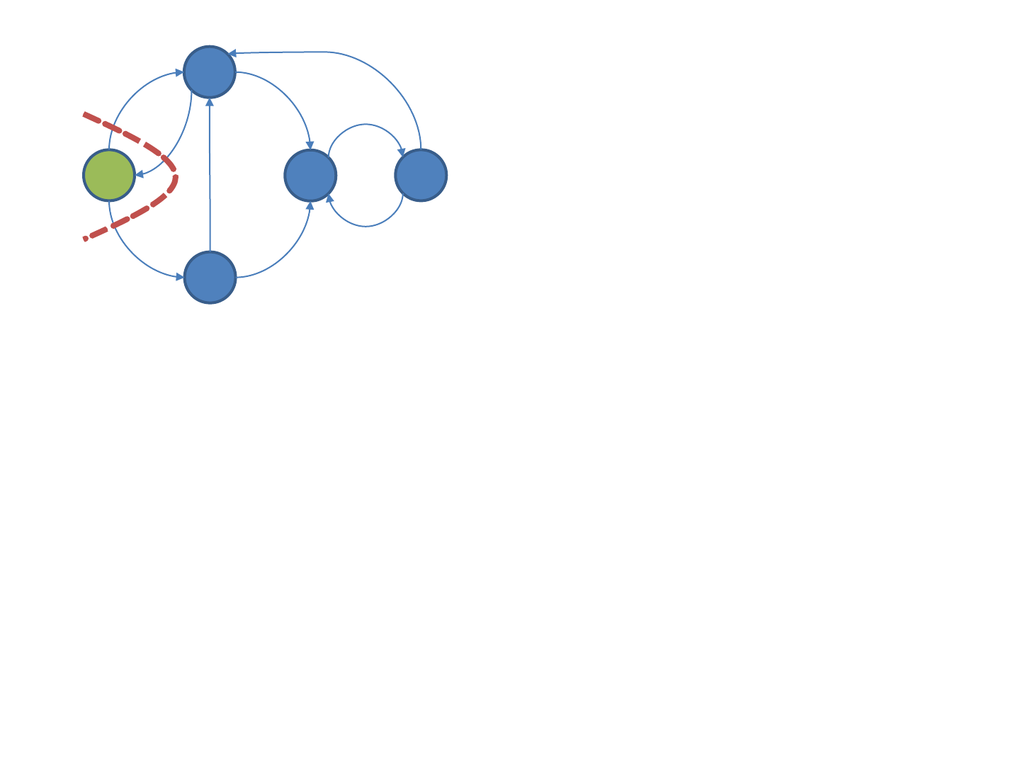
When to Stop Iterating
• How does the algorithm know when all shortest paths were found?
• If all edges have the same weight, stop iterating as soon as no vertex has distance
∞ any more: Later iterations can only find longer paths. This can be detected using
a global counter or accumulator.
– The number of iterations depends on the graph diameter. In practice, social networks often
show the small-world phenomenon, i.e., have a small diameter.
• If edges have different weights, then a “detour” path can have a lower total weight
than a more “direct” connection and hence we cannot stop as soon as all vertex
distances are finite. Instead, iterations must continue until no shortest distance
changes. This can also be detected using a global counter or accumulator.
– In the worst case, this takes |V|-1 iterations, where |V| is the number of graph vertices.
• In a graph with cycles of negative weight the algorithm never terminates: each
traversal of the cycle reduces the distances of all its vertices indefinitely.
59
s
a
b
c
d
18
9
7
6
1
3
2
5
4
This is an example for a graph where a “detour”
path consisting of four edges is shorter than the
direct path. Path (s, a) has length 18, while path
(s, b, c, d, a) has length 15. Detecting this
shortest path requires 4 iterations.

Single-Source Shortest Path in MapReduce
• The algorithm is virtually identical to BFS, but also
keeps track of the shortest distance found for
each vertex so far:
– Map processes a single vertex u, emitting
d[u]+weight(u,v) for each vertex v in u’s adjacency list.
– Reduce collects the newly computed distances for all
inlinks of vertex v and determines if any of them is
shorter than its currently known shortest distance.
• The driver program repeatedly calls the
MapReduce program as many times as necessary,
exploring ever longer paths.
60

MapReduce Code for a Single Iteration
61
// The vertex object now also contains the
// current min distance and edges in the
// adjacency list have a weight
map(vertex N) {
// Pass along the graph structure
emit(N.id, N)
// Compute the distance for each outlink
for all m in N.adjacencyList do
emit( m, N.distance + weight(n,m) )
}
// Reduce receives the vertex object for vertex m and
// the newly computed distances for m’s inlinks
reduce(id m, [d1, d2,…]) {
dMin = ∞
M = NULL
for all d in [d1, d2,…] do
if isVertex(d) then
// The vertex object was found: recover graph structure
M = d
else
// A distance value for an inlink was found: keep track
// of the minimum.
if d < dMin then dMin = d
// Update distance of vertex m if necessary.
if dMin < M.distance then M.distance = dMin
emit( m, M )
}

MapReduce Algorithm Analysis
• Each iteration of the algorithm performs a large amount of work:
– The entire graph is read from the distributed file system, transferred
from Mappers to Reducers, and then, with updated distance values,
written to the distributed file system.
– For every vertex u, no matter if it potentially lies on a shorter path to
another vertex v or not, distance d[u]+weight(u,v) is computed and
sent to the Reducers.
– For every vertex v, no matter if its shortest path was already found in
previous iterations or not, the Reduce function is executed to re-
compute the shortest distance.
• This brute-force approach performs many irrelevant computations:
– In early iterations, Map computes distances for vertices that have not
yet been reached, therefore still have infinity distance.
– In later iterations, the program keeps re-computing paths for vertices
whose shortest path was already found.
• Contrast this with the elegance of Dijkstra’s algorithm, which avoids
this irrelevant computation, but needed the priority queue in order
to achieve this.
62

Improving the MapReduce Algorithm:
Avoiding Useless Work
• Can we avoid processing vertices that do not improve any distances in the
iteration? This turns out to be easy based on the following observations:
– If a vertex u has distance d[u]=∞, then it cannot help reduce the distance for
any of the vertices in its adjacency list.
– Assume vertex u had the same distance d[u]=x in iterations i and (i+1). For any
vertex v in its adjacency list, the Map function call for u would emit the same
value x+weight(u,v) in both iterations. Since this value was already included in
the Reduce computation in iteration i, it cannot result in improvements in
iteration (i+1).
• To exploit these properties, we can do the following:
– Like BFS, the program distinguishes between “active” and “inactive” vertices.
Active vertices are those that could potentially help reduce the distance for
another vertex. We define a vertex to be active if and only if its distance value
changed in the previous iteration. The only exception to this rule is source
vertex s, which is set to “active” before the first iteration. Note that a vertex
that was active in one iteration could become inactive in the next, and vice
versa.
– It is easy to prove that a vertex whose distance reached the final value, i.e.,
the shortest-path distance from s, will remain inactive afterwards. Hence the
algorithm can stop iterating as soon as all vertices become inactive.
• The corresponding program is shown next.
63

Improved MapReduce Code for a Single
Iteration
64
// The vertex object now also keeps track
// if the vertex is active.
map( vertex N ) {
// Pass along the graph structure
emit(N.id, N)
// Compute the distance for each outlink
// of an active vertex
if N.isActive {
for all m in N.adjacencyList do
emit( m, N.distance + weight(n,m) )
}
}
// Reduce receives the vertex object for vertex m and
// the newly computed distances for m’s inlinks
reduce(id m, [d1, d2,…]) {
dMin = ∞; M = NULL
for all d in [d1, d2,…] do
if isVertex(d) then
// The vertex object was found: recover graph structure
M = d
else
// A distance value for an inlink was found: keep track
// of the minimum.
if d < dMin then dMin = d
// Update distance of vertex m if necessary.
if dMin < M.distance then {
M.distance = dMin
// The distance change can affect the distance for
// nodes in the adjacency list, hence set status to active
M.setActive(true)
}
emit( m, M )
}

Single-Source Shortest Path in Spark
• We discuss the Spark Scala pseudo-code with RDDs.
The version with DataSet is left as a voluntary
challenge.
• The Spark program separates static data (the graph
structure) from evolving data (the currently known
shortest distance of each vertex).
– This leverages cached RDD partitions and avoids the
shuffling of the adjacency list data we saw in the
MapReduce implementation.
– On the downside, the new distance-status information
must be combined with the graph data, so that tuples of
type (vertexID, adjacencyList) and (vertexID, distance) are
joined on vertexID. This join normally requires shuffling,
but careful co-partitioning avoids shuffling.
65

Spark Implementation
66
// Each line in the input file contains a vertex ID and its adjacency list. Function getAdjListPairData returns
// a pair (vertex ID, adjacency list), creating a pair RDD. An entry in the adjacency list is a pair of destination
// vertex id and edge weight. The source node’s adjacency list has a special “source” flag for setting of
// the initial distances.
graph = sc.textFile(…).map( line => getAdjListPairData(line) )
// Add code here to make sure the graph has a Partitioner. This avoids shuffling in the join below.
// Tell Spark to try and keep this pair RDD in memory for efficient re-use
graph.persist()
// Create the initial distances. mapValues ensures that the same Partitioner is used as for the graph RDD.
distances = graph.mapValues( (id, adjList) => hasSourceFlag(adjList) match {
case true => 0
case _ => infinity }
// Function extractVertices returns each vertex id m in n’s adjacency list as (m, distance(n)+w),
// where w is the weight of edge (n, m). It also returns n itself as (n, distance(n))
for (iterationCount <- 1 to k) { // Use Accumulator instead to determine when last iteration is reached
distances = graph.join( distances )
.flatMap( (n, adjList, currentDistanceOfN) => extractVertices(adjList, currentDistanceOfN) )
.reduceByKey( (x, y) => min(x, y) ) // Remember the shortest of the distances found
}

Single-Source Shortest Path in a DBMS
• Assume the graph is stored in table Graph(id1, id2,
weight) and the currently known shortest distances in
table Distances(id, distance), where id1, id2, and id are
all vertex IDs. Then we can express the computation of
an iteration as shown below.
67
tempDistances =
SELECT G.id2 AS id, D.distance+G.weight AS distance
FROM Graph AS G, Distances AS D
WHERE G.id1 = D.id
UNION
SELECT * FROM Distances
newDistances =
SELECT id, min(distance)
FROM tempDistances
GROUP BY id

68
We now explore the famous PageRank
(PR) algorithm.
Compare and contrast the parallel version
to SSSP.

PageRank
• PageRank was popularized by Google as a measure for evaluating
the importance of a Web page. Intuitively it assigns greater
importance to pages that are linked from many other important
pages.
• PageRank captures the probability of a “random Web surfer”
landing on a given page. The random Web surfer can reach a page
by jumping to it or by following the link from another page pointing
to it.
• PageRank helps identify the most relevant results for a keyword
query. For example, consider query “Northeastern University.” A
person entering these keywords will most likely be looking for the
Northeastern.edu homepage. If a search engine only considers
traditional measures of importance such as TF/IDF, it might highly
rank a spam page containing term “Northeastern” many times.
Assuming that Northeastern.edu will be linked from many more
important pages than the spam site, taking into account the
PageRank value can help boost its rank in the result list.
69

PageRank Definition
• The importance of a Web page is measured by the probability that a
random Web surfer will land on it. They can reach a page either by typing
a random URL into the browser’s address field (aka perform a random
jump) or by following a random link from the page they currently visit. The
probability of doing the latter is α.
• Formally,
, where
– |V| is the number of pages (vertices) in the Web graph considered.
– is the probability of the surfer following a link (vs. 1-α for a random jump).
– L(n) is the set of all pages in the graph linking to n.
– P(m) is the PageRank of another page m.
– C(m) is the out-degree of page m, i.e., the number of links on that page.
• The 2 main terms in the formula correspond to the 2 ways of reaching n:
– The random surfer reaches it via a random jump if they (1) decide to make a
random jump (probability 1-α) and (2) choose exactly this 1 out of |V|
possible Web pages.
– They reach it via a link if they (1) decide to follow a link (probability α), (2)
were visiting another page m (which they happen to be currently visiting with
probability P(m)) that links to n, and (3) selected the 1 out of C(m) links on m
pointing to n.
70

Iterative PageRank Computation
• Notice that the definition of PageRank creates a
“chicken-and-egg problem”:
– To compute the PageRank of page n, we need to know the
PageRank of all other pages linking to it, which in turn
might depend on n’s PageRank.
• Fortunately, this recursive definition admits an iterative
algorithm for computing all PageRank values in the
graph. Starting with some initial values, each iteration
computes the new PageRank for all pages. This process
continues until a fixpoint is reached, meaning that the
value for every page does not change any more.
• Let’s look at an example to see PageRank iterations in
action.
71

Initial State
72
0.2
0.2
0.2
0.2
0.2
Assume that all PageRank values are initialized to 0.2. For simplicity we set α=1, i.e.,
the random surfer only follows links.

Iteration 1: PageRank Transfer
73
0.2
0.2
0.2
0.2
0.2
0.1
0.1
0.1
0.1
0.1
0.1
0.2
0.1
0.1
Since α=1, each page passes on its full PageRank value, distributed equally over the
outgoing links.

Iteration 1: Updated PageRank
74
0.1
0.3
0.1
0.3
0.2
It is clearly visible how some pages receive more weight than others.

Iteration 2: PageRank Transfer
75
0.1
0.3
0.1
0.3
0.2
0.05
0.05
0.05
0.05
0.15
0.15
0.3
0.1
0.1
Since α=1, each page again passes on its full PageRank value along the outgoing links.

Iteration 2: Updated PageRank
76
0.15
0.2
0.05
0.3
0.3
Already after two iterations, major properties of the algorithm show. First, from
iteration to iteration, the PageRank of a page can oscillate between higher and lower
values. E.g., the leftmost page changed from 0.2 to 0.1, then to 0.15. Over time, these
changes become smaller as the values converge. Second, despite the oscillations, the
general tendency is for some pages to accumulate larger values, while others drop.

PageRank using BFS
• Observing the steps during an iteration of PageRank, it
becomes clear that there are two phases. In the first
phase of the iteration, a page sends out fractions of its
current PageRank along its outgoing edges. In the
second phase, each page sums up the PageRank
contributions along all its incoming edges.
• Given page n’s current value P(n) and adjacency list,
one can compute all its outgoing contributions.
• Adding the incoming contributions for page m requires
re-shuffling.
– The term (1-α)/|V| remains constant throughout the
computation. Both α and |V| can be shared with all tasks.
• Interestingly, the computation pattern again matches
BFS.
77

PageRank in MapReduce
• The algorithm is virtually identical to BFS, but
an iteration must also keep track of the
current PageRank value of each page:
– Map processes a single vertex n, emitting the
PageRank of n, divided by n’s outdegree, for each
vertex m in n’s adjacency list.
– Reduce collects PageRank contributions from all
inlinks of vertex m and then applies the formula.
• The driver program repeatedly calls the
MapReduce program until (near) convergence,
i.e., when all PageRank values stabilize.
78

MapReduce Code for a Single Iteration
79
// The vertex object now also stores
// the current PageRank value
map( vertex N ) {
// Pass along the graph structure
emit(N.id, N)
// Compute contributions to send
// along outgoing links
p = N.pageRank / N.adjacencyList.size()
for all m in N.adjacencyList do
emit( m, p )
}
// Reduce receives the vertex object for vertex m and
// the PageRank contributions for all m’s inlinks
reduce(id m, [p1, p2,…]) {
s = 0
M = NULL
for all p in [p1, p2,…] do
if isVertex(p) then
// The vertex object was found: recover graph structure
M = p
else
// A PageRank contribution from an inlink was found:
// add it to the running sum.
s += p
M.pageRank = (1-)/|V| + s
emit( m, M )
}

MapReduce Algorithm Analysis
• A careful look reveals that this program is structurally
almost identical to the one for single-source shortest
path. Hence it shares the same weaknesses caused by
MapReduce’s inability to exploit repetitive structure in
iterative programs. In each iteration:
– The entire graph is read from the distributed file system.
– The entire graph is transferred from Mappers to Reducers.
– The entire graph, with updated PageRank values, is written
to the distributed file system.
• On the other hand, the PageRank program does not
perform irrelevant computation. In contrast to single-
source shortest path, all PageRank values must be
recomputed in every iteration.
80

PageRank in Spark
• We discuss the Spark Scala pseudo-code with RDDs. The
version with DataSet is left as a voluntary challenge.
• The Spark program separates static data (the graph
structure) from evolving data (the current PageRank of
each vertex).
– This leverages cached RDD partitions and avoids MapReduce’s
shuffling of the adjacency list data.
– On the downside, the new PageRank data of type (vertexID,
PageRank) must be joined with the graph data of type (vertexID,
adjacencyList). This join on vertexID normally requires shuffling,
but careful co-partitioning avoids that.
• Look at the program from the Spark 2.4.0 distribution at
http://khoury.northeastern.edu/home/mirek/code/SparkP
ageRank.scala
– Notice that it does not handle dangling pages.
81

Simplified Spark Implementation
82
// The input file contains in each line a vertex ID and its adjacency list. Function
// getAdjListPairData returns a pair of vertex ID and its adjacency list, creating a pair RDD.
graph = sc.textFile(…).map( line => getAdjListPairData(line) )
// Add code here to make sure that the graph pair RDD has a Partitioner.
// This is needed for avoiding shuffling in the join below.
// Tell Spark to try and keep this pair RDD around in memory for efficient re-use
graph.persist()
// Create the initial PageRanks using page count |V|, which can be passed through the context.
// Function mapValues ensures that the same Partitioner is used as for the graph RDD.
PR = graph.mapValues( adjList => 1.0 / |V| )
// Function extractVertices returns each vertex id m in n’s adjacency list as
// (m, n’s PageRank / number of n’s outlinks).
for (iterationCount <- 1 to k) { // Use Accumulator instead to detect (approximate) convergence
PR = graph.join( PR )
.flatMap( (n, adjList, currentPRofN) => extractVertices(adjList, currentPRofN) )
.reduceByKey( (x, y) => (x + y) ) // Add PageRank contributions
}

Another Spark PageRank Program
• The next example is a complete Spark Scala
program from a Spark textbook. The authors set
=0.85, following the original PR paper.
• Take a moment and compare the two PR
programs. What is different, what is the same?
• Notice how |V|, the number of Web pages, does
not appear in the second program. Initial PR
values are set to 1.0 and the updated PR is
0.15+0.85*incoming_PR_contributions.
– Convince yourself that this is equivalent to computing
the true PR values, just multiplied by |V|.
83

Code Fragment from Learning Spark by
Zaharia et al.
84
// Assume that our neighbor list was saved as a Spark objectFile
val links = sc.objectFile[(String, Seq[String])]("links").partitionBy(new HashPartitioner(100))
.persist()
// Initialize each page's rank to 1.0; since we use mapValues, the resulting RDD
// will have the same partitioner as links
var ranks = links.mapValues(v => 1.0)
// Run 10 iterations of PageRank
for (i <- 0 until 10) {
val contributions = links.join(ranks).flatMap {
case (pageId, (links, rank)) => links.map(dest => (dest, rank / links.size))
}
ranks = contributions.reduceByKey((x, y) => x + y).mapValues(v => 0.15 + 0.85*v)
}
// Write out the final ranks
ranks.saveAsTextFile("ranks")

85
Let us look at the key difference between
Spark and MapReduce.

86
Typical iterative job (PageRank) in Hadoop MapReduce:
GraphPR(pageID,
adjacency list,
PRvalue)
In MapReduce, each input record in GraphPR contains both the adjacency
list and the PageRank value for each page. The PageRank algorithm iterates
through the entire graph to update these PRvalues.

87
Typical iterative job (PageRank) in Hadoop MapReduce:
GraphPR(pageID,
adjacency list,
PRvalue)
Worker
(map)
Worker
(map)
Worker
(map)
Worker
(map)
Graph
PR
The MapReduce program first loads the Graph with its PRvalues into the
Mappers. (Graph and PRvalue data are shown separately for better
comparability to the Spark approach.)

88
Typical iterative job (PageRank) in Hadoop MapReduce:
GraphPR(pageID,
adjacency list,
PRvalue)
Worker
(map)
Worker
(reduce)
Worker
(map)
Worker
(map)
Worker
(map)
Worker
(reduce)
Worker
(reduce)
Worker
(reduce)
Graph
PR
Graph
PR up-
dates
Each Mapper forwards graph structure and update info for the PRvalues to
the corresponding Reducers.

89
Typical iterative job (PageRank) in Hadoop MapReduce:
GraphPR(pageID,
adjacency list,
PRvalue)
Worker
(map)
Worker
(reduce)
Worker
(map)
Worker
(map)
Worker
(map)
Worker
(reduce)
Worker
(reduce)
Worker
(reduce)
Graph
PR
Graph
Graph
new
PR
PR up-
dates
Per-iteration flow
The Reducers compute the new PRvalues and emit the updated graph to the
distributed file system.
This cycle repeats in the next iteration.

90
Typical iterative job (PageRank) in Spark:
Graph(pageID,
adjacency list),
PR(pageID, value)
Spark manages data that changes in each iteration (PR: the PageRank value
of a page) separate from data that does not (Graph: the graph structure, i.e.,
the pages and their adjacency lists of links.) This enables it to exploit in-
memory data and dramatically reduce data movement.

91
Typical iterative job (PageRank) in Spark:
Graph(pageID,
adjacency list),
PR(pageID, value)
Worker
(map)
Worker
(map)
Worker
(map)
Worker
(Spark
executor)
Graph
PR
One-time flow Per-iteration flow
First, both Graph and PR are loaded into the Spark worker tasks. Ideally
(when the graph fits into the combined memory of all tasks) this initial
loading step happens only once, not in each iteration.

92
Typical iterative job (PageRank) in Spark:
Graph(pageID,
adjacency list),
PR(pageID, value)
Worker
(map)
Worker
(map)
Worker
(map)
Worker
(Spark
executor)
Graph
PR
PR up-
dates
One-time flow Per-iteration flow
Since the workers can keep the Graph data as an RDD or DataSet in memory,
Graph does not need to be loaded and saved repeatedly. Instead, each
iteration only passes the PR value updates to the task processing the
corresponding node.

93
Typical iterative job (PageRank) in Spark:
Graph(pageID,
adjacency list),
PR(pageID, value)
Worker
(map)
Worker
(map)
Worker
(map)
Worker
(Spark
executor)
Graph
PR
new
PR
PR up-
dates
Driver
One-time flow Per-iteration flow
In the very end, the final PR values are collected by the driver. This again is a
one-time data transfer, not one happening in each iteration.

94
Typical iterative job (PageRank) in Spark:
Graph(pageID,
adjacency list),
PR(pageID, value)
Worker
(map)
Worker
(map)
Worker
(map)
Worker
(Spark
executor)
Graph
PR
new
PR
PR up-
dates
Driver
new
PR
One-time flow Per-iteration flow
The driver then saves the final PR values to the distributed file system.

95
PageRank in Hadoop MapReduce:
PageRank in Spark:
GraphPR(pageID,
adjacency list,
PRvalue)
Worker
(map)
Worker
(reduce)
Worker
(map)
Worker
(map)
Worker
(map)
Worker
(reduce)
Worker
(reduce)
Worker
(reduce)
Graph
PR
Graph
Graph
new
PR
PR up-
dates
Graph(pageID,
adjacency list),
PR(pageID, value)
Worker
(map)
Worker
(map)
Worker
(map)
Worker
(Spark
executor)
Graph
PR
new
PR
PR up-
dates
Driver
new
PR
One-time flow Per-iteration flow

PageRank in a DBMS
• Assume the graph is stored in table Links(origin,
destination) and the PageRank values in table
PageRank(pageID, PR, outDegree), where origin,
destination, and pageID are vertex IDs, and outdegree
is the number of vertices in the adjacency list of vertex
pageID. Then we can express the computation of an
iteration as shown below.
96
newPR = SELECT L.destination, (1-alpha)*numPages + alpha*SUM(P.PR/P.outDegree)
FROM Links AS L, PageRank AS P
WHERE L.origin = P.pageID
GROUP BY L.destination
(Note that numPages = SELECT COUNT(*) FROM PageRank.)

Dangling Pages
• Dangling pages, i.e., pages that have no outgoing links, leak
PageRank probability mass. Consider a dangling page x with
PageRank P(x). During an iteration, P(x) is not passed along to
another page and hence probability mass αP(x) disappears. Stated
differently, dangling pages cause the total PageRank sum of the
graph to decrease with every iteration.
• How can we address this problem? If the random surfer ends up on
a dangling page, she cannot follow links and hence must perform a
random jump. We model this mathematically by conceptually
adding imaginary links from x to every page in the graph, including x
itself. If we use δ to denote the total PageRank mass of dangling
pages, then the corresponding formula for the PageRank of page n
becomes
• Since PageRank values of dangling pages may change, we must
compute the new value of in each iteration.
97

Dangling-Pages Solution in MapReduce
• The formula computing the new PageRank in Reduce
must be modified to include the term with variable δ.
• Unfortunately, it is not possible to compute some value
and also read it out in the same MapReduce job. We
next discuss multiple possible solutions in more detail.
• Solution 1: add a separate job to each iteration to
compute δ.
– During an iteration, first execute a MapReduce job that
computes δ. This is a simple global aggregation job,
summing up PageRank values for all dangling pages.
– Then pass the newly computed δ as a parameter to the
modified MapReduce program that updates all PageRanks
using the new formula with δ.
• Can we avoid the extra job in each iteration?
98

Alternative Solutions
• Solution 2: global counter.
– We can compute δ “for free” during the Map phase. When Map
processes a node with an empty adjacency list, it adds the node’s
PagePank to a global counter. By the end of the Map phase, this
counter’s value is . If Reducers can read the counter value, they can
compute the correct new PageRank in the Reduce function.
Otherwise, the global counter is read in the driver after the job
completed. The driver then passes its value via the context to the next
iteration’s Map phase.
• Solution 3: dummy page.
– For a dangling page n, the Map function emits (dummy, n’s PageRank).
The Reduce call for the dummy node then adds up all contributions.
The driver reads this output and passes it into the next job’s context.
• Solution 4: order inversion.
– In Map, the page’s PageRank is the old value computed in the previous
iteration i. Reduce computes the new value output in iteration i+1.
Hence we can apply the order inversion design pattern to send each
Reducer the old PageRank values of all dangling pages, allowing it to
compute δ right before executing the “normal” Reduce calls.
99

Solution 2 Pseudo-Code (May Not Work!)
100
map( vertex N ) {
// Pass along the graph structure
emit(N.id, N)
// Compute contributions to send
// along outgoing links
s = N.adjacencyList.size()
if (s>0) {
p = N.pageRank / s
for all m in N.adjacencyList do
emit( m, p )
} else // dangling page
global_counter.add( N.PageRank )
}
// Reduce receives the vertex object for vertex m and
// the PageRank contributions for all m’s inlinks
reduce(id m, [p1, p2,…]) {
s = 0
M = NULL
for all p in [p1, p2,…] do
if isVertex(p) then
// The vertex object was found: recover graph structure
M = p
else
// A PageRank contribution from an inlink was found:
// add it to the running sum.
s += p
// This only works if Reducers can read global counters
M.pageRank = (1-)/|V| + (global_counter/|V| + s)
emit( m, M )
}

Solution 2 Discussion
• That program may not work in practice. By design, a global counter
is initialized in the driver, updated by Map and Reduce tasks, then
read out in the driver after the job completed.
• The above program needs to read the counter value in the
Reducers. In theory this could be supported, because of the barrier
between Map and Reduce phase: no Reducer can start processing
its input until all Mappers have finished (and hence finished
updating the counter).
• In practice, the implementation of the counter feature may not
guarantee the global count to be stable and finalized until the entire
job has finished. This needs to be verified based on the MapReduce
documentation.
• The following program is an alternative where the counter value is
passed via the job context to the next iteration.
– Note that the output of the last iteration is not corrected for the
dangling PageRank mass. To do so would require another Map-only
job for cleanup.
101

Solution 2 Pseudo-Code
102
map( vertex N ) {
// Update PageRank using from previous
// iteration, passed from the driver via the
// job context; = 0 in the first iteration
N.pageRank += / |V|
// Pass along the graph structure
emit(N.id, N)
// Compute contributions to send
// along outgoing links
s = N.adjacencyList.size()
if (s>0) {
p = N.pageRank / s
for all m in N.adjacencyList do
emit( m, p )
} else // dangling page
global_counter.add( N.PageRank )
}
// Reduce receives the vertex object for vertex m and
// the PageRank contributions for all m’s inlinks
reduce(id m, [p1, p2,…]) {
s = 0
M = NULL
for all p in [p1, p2,…] do
if isVertex(p) then
// The vertex object was found: recover graph structure
M = p
else
// A PageRank contribution from an inlink was found:
// add it to the running sum.
s += p
// This PageRank value does not account for dangling
// PageRank mass yet!
M.pageRank = (1-)/|V| + s
emit( m, M )
}
The driver reads the global counter’s value after the job
completes, passing it to the job for the next iteration.

Dangling-Pages Solution in Spark
• The Spark solutions mirror those in MapReduce.
– We can compute the dangling PageRank mass in a separate step.
– Instead of a global counter, we can use an Accumulator to compute the
dangling mass in iteration i, then use it in iteration (i+1).
– We can also add the dummy page to the graph RDD, accessing its PR value
using lookup.
• All these solutions add an action: the separate computation step uses a
global aggregate on the RDD, Accumulator access is an action, and so is
the lookup operation.
– This action forces a Spark-job execution for each iteration. Instead, it would be
more efficient to run a single Spark job that executes all iterations.
– Notice that the dangling-page-related action in iteration i depends on the
PageRanks and the dangling PR mass in iteration (i-1). Those in turn depend
on iteration (i-2), etc. This creates lineage information that is quadratic in the
number of iterations j: The PR values from iteration 1 appear in the lineage of
iterations 2,…, j; those from iteration 2 appear in 3,…, j; etc.
– Challenge question: Since the PageRanks from iteration 1 are needed by the j-
1 jobs triggered in later iterations, does this mean iteration 1 will be executed j
times (and similarly the second iteration j-1 times, etc)? Would persisting the
PageRanks RDD change this behavior?
103

Dangling-Pages Solution in a DBMS
• In SQL, we create an intermediate table with the dangling
PageRank mass and rely on the optimizer to find an
efficient computation strategy.
– Note that for dangling pages n, there is no tuple with origin=n in
Links. Hence we find all dangling pages by checking for page IDs
that do not appear in the origin column in Links.
104
dangling = SELECT SUM(PR)
FROM PageRank
WHERE id NOT IN
(SELECT origin FROM Graph)
newPR = SELECT L.destination,
(1-alpha)*numPages + alpha*(dangling / numPages + SUM(P.PR/P.outDegree))
FROM Links AS L, PageRank AS P
WHERE L.origin = P.pageID
GROUP BY L.destination

Number of Iterations
• In theory, the computation terminates when the fixpoint is reached, i.e.,
none of the PageRank values changes from one iteration to the next. In
practice approximate numbers suffice, therefore iterations can stop as
soon as all PageRank values “barely change.”
– It is often reasonable to stop when no page’s PageRank changes by more than
1%. This threshold for relative change is computed for each page n as |new(n)
– old(n)| / old(n), where old(n) and new(n) are the PageRank of n in previous
and current iteration, respectively.
– A threshold for absolute change |new(n) – old(n)| is difficult to set, because
PageRank values can vary by multiple orders of magnitude in large graphs.
• The easiest way to check for convergence is via a global counter or
Accumulator that determines for how many pages the PageRank change
was greater than the threshold. The counter is updated in the Reduce
function (or the corresponding Spark function), where both old and new
PageRank of a page are available. The driver program then checks the
counter value to decide about another iteration.
• Depending on graph size, structure, and convergence threshold, the
number of iterations can vary widely. The paper that proposed PageRank
reported convergence after 52 iterations for a graph with 322 million
edges.
105

Summary
• Large graphs tend to be sparse and hence are often stored in
adjacency-list or set-of-edges format. This representation enables
per-vertex computation in a single round, which can pass
information along outgoing edges to all direct neighbors.
– It is possible to extend this capability by pre-computing other data
structures, e.g., the list of neighbors within a certain distance, to push
information directly to nodes farther away.
• Computation along incoming edges requires shuffling.
• The driver program controls execution of iterations, until a stopping
condition is met.
• For some problems, the most efficient or most elegant sequential
algorithms rely on a “centralized” data structure. These algorithms
are difficult to parallelize directly.
• Iterative algorithms are common in practice and can be
implemented easily in MapReduce and Spark. However,
MapReduce’s lack of support for persistent in-memory data results
in inefficiencies due to costly data transfer.
106

Summary (Cont.)
• Each iteration of the presented algorithms has linear time
complexity in graph size, scaling to large graphs.
• For algorithms that push data along graph edges, shuffle
cost in Spark depends on the number of edges “across
partitions.” (We discuss this on the next pages.) A good
partitioning therefore keeps densely connected regions of
the graph together, cutting through sparse ones.
Unfortunately, finding a balanced min-cut-style graph
partitioning is hard.
• Big data raises the issue of numerical stability: In a billion-
vertex graph an individual PageRank could underflow
floating-point precision. Careful analysis is needed to
decide if a number type of greater precision suffices or if a
numerically more robust algorithm should be used. For
instance, since log(x·y)=log(x)+log(y), one can replace
multiplication by addition of log-transformed numbers.
107

Side-Note: Graph Partitions versus
Communication
• Consider the PageRank algorithm in Spark,
where the graph RDD is partitioned over the
different tasks. After loading the graph for the
first iteration, no further graph-data
movement occurs.
• However, PageRank values still change and
need to be passed along outgoing edges to be
aggregated along incoming edges.
• Consider the following example partitioning,
showing the adjacency lists managed by each
task.
108

Partitions versus Communication
109
1
2
3
4
5
6 7
8
Graph partitions:
Partition A:
node 1: 2
node 2: 1, 3, 4
node 3: 1, 6
Partition B:
node 4: 5
node 5: 4
Partition C:
node 6: 7
node 7: 5, 6
node 8: 6, 7

Partitions versus Communication
• During an iteration of the PageRank computation,
each vertex sends its contributions along the
outgoing edges. For destination vertices in the
same partition, data transfer is local (indicated by
a blue arrow on the next page).
• To avoid costly network transfer, the graph should
be partitioned such that the number of edges
connecting vertices in different partitions is
minimized. In the example, only three edges
(shown in red) require data transfer to a different
task. After receiving the incoming contributions,
for each vertex the new PageRank can be
computed.
110
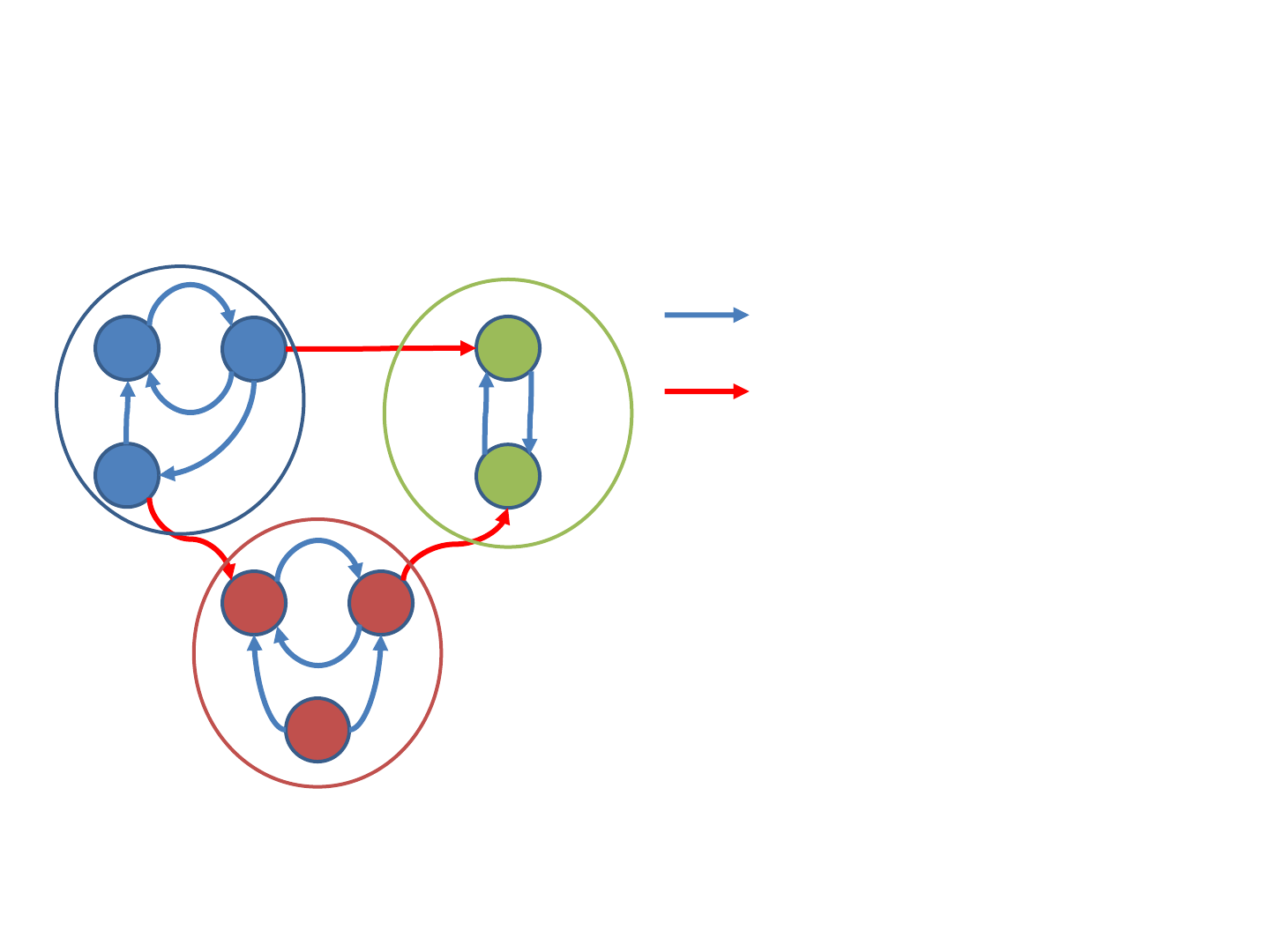
Efficient Iterative Processing
111
1
2
3
4
5
6 7
8
PageRank mass transfer:
local transfer
transfer to a different task

