
Graphs
Computer Science S-111
Harvard University
David G. Sullivan, Ph.D.
Unit 10
• A graph consists of:
• a set of vertices (also known as nodes)
• a set of edges (also known as arcs), each of which connects
a pair of vertices
What is a Graph?
vertex / node
edge / arc
e
b d f h
j
a
c
i
g

• Vertices represent cities.
• Edges represent highways.
• This is a weighted graph, with a cost associated with each edge.
• in this example, the costs denote mileage
• We’ll use graph algorithms to answer questions like
“What is the shortest route from Portland to Providence?”
Example: A Highway Graph
Portland
Portsmouth
Boston
Concord
Albany Worcester
Providence
New York
39
54
44
83
49
42
185
134
63
84
74
• Two vertices are adjacent if they are connected by a single edge.
• ex: c and g are adjacent, but c and i are not
• The collection of vertices that are adjacent to a vertex v are
referred to as v’s neighbors.
• ex: c’s neighbors are a, b, d, f, and g
Relationships Among Vertices
e
b d f h
j
a
c
i
g

• A path is a sequence of edges that connects two vertices.
• A graph is connected if there is
a path between any two vertices.
• ex: the six vertices at right are part
of a graph that is not connected
• A graph is complete if there is an
edge between every pair of vertices.
• ex: the graph at right is complete
Paths in a Graph
e
b d f h
j
a
c
i
g
• A directed graph has a direction associated with each edge,
which is depicted using an arrow:
• Edges in a directed graph are often represented as ordered
pairs of the form (start vertex, end vertex).
• ex: (a, b) is an edge in the graph above, but (b, a) is not.
• In a path in a directed graph, the end vertex of edge i
must be the same as the start vertex of edge i + 1.
• ex: { (a, b), (b, e), (e, f) } is a valid path.
{ (a, b), (c, b), (c, a) } is not.
Directed Graphs
e
b d f
a
c

• A cycle is a path that:
• leaves a given vertex using one edge
• returns to that same vertex using a different edge
• Examples: the highlighted paths below
• An acyclic graph has no cycles.
Cycles in a Graph
e
b d f h
a
c
i
• A tree is a special type of graph.
• connected, undirected, and acyclic
• we usually single out one of the vertices to be the root,
but graph theory does not require this
a graph that is not a tree, a tree using the same nodes
because it has cycles
another tree using the same nodes
Trees vs. Graphs
e
b d f h
a
c
i
e
b d f h
a
c
i
e
b d f h
a
c
i

• A spanning tree is a subset of a connected graph that contains:
• all of the vertices
• a subset of the edges that form a tree
• Recall this graph with cycles
from the previous slide:
• The trees on that slide were spanning trees for this graph.
Here are two others:
Spanning Trees
e
b d f h
a
c
i
e
b d f h
a
c
i
e
b d f h
a
c
i
Representing a Graph: Option 1
• Use an adjacency matrix – a two-dimensional array in which
element [r][c] = the cost of going from vertex r to vertex c
•Example:
• Use a special value to indicate there’s no edge from r to c
• shown as a shaded cell above
• can’t use 0, because an edge may have an actual cost of 0
• This representation:
• wastes memory if a graph is sparse (few edges per vertex)
• is memory-efficient if a graph is dense (many edges per vertex)
0123
0 54 44
1 39
2 54 39 83
3 44 83
1. Portland
2. Portsmouth
0. Boston3. Worcester
54
44
83
39

Representing a Graph: Option 2
• Use one adjacency list for each vertex.
• a linked list with info on the edges coming from that vertex
• This representation uses less memory if a graph is sparse.
• It uses more memory if a graph is dense.
• because of the references linking the nodes
3
44
0
1
2
3
2
54
null
2
39
null
1
39
0
44
2
83
null
1. Portland
2. Portsmouth
0. Boston3. Worcester
39
54
44
83
3
83
null
0
54
Graph Class
public class Graph {
private class Vertex {
private String id;
private Edge edges;
// adjacency list
private Vertex next;
private boolean encountered;
private boolean done;
private Vertex parent;
private double cost;
…
}
private class Edge {
private Vertex start;
private Vertex end;
private double cost;
private Edge next;
…
}
private Vertex vertices;
…
}
The highlighted fields
are shown in the diagram
on the previous page.

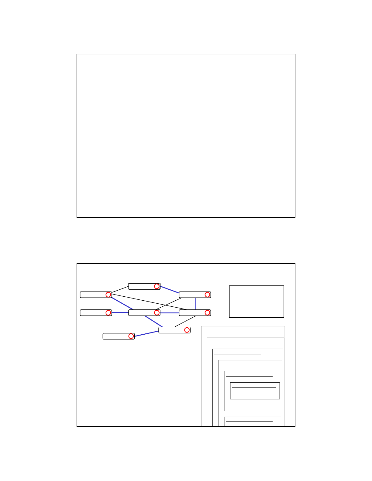
Our Graph Representation
• Each Vertex object (shown in blue) stores info. about a vertex.
• including an adjacency list of Edge objects (the purple ones)
• A Graph object has a single field called vertices
• a reference to a linked list of Vertex objects
• a linked list of linked lists!
44
null
54
null
39
39 54
44
null
83
“Boston”
“Portland”
“Portsmouth”
null
“Worcester”
vertices
Portland
Portsmouth
BostonWorcester
39
54
44
83
83
null
Traversing a Graph
• Traversing a graph involves starting at some vertex and visiting
all vertices that can be reached from that vertex.
• visiting a vertex = processing its data in some way
• if the graph is connected, all of its vertices will be visited
• We will consider two types of traversals:
• depth-first: proceed as far as possible along a given path
before backing up
• breadth-first: visit a vertex
visit all of its neighbors
visit all unvisited vertices 2 edges away
visit all unvisited vertices 3 edges away, etc.
• Applications:
• determining the vertices that can be reached from some vertex
• web crawler (vertices = pages, edges = links)
Depth-First Traversal
• Visit a vertex, then make recursive calls on all of its
yet-to-be-visited neighbors:
dfTrav(v, parent)
visit v and mark it as visited
v.parent = parent
for each vertex w in v’s neighbors
if (w has not been visited)
dfTrav(w, v)
• Java method:
private static void dfTrav(Vertex v, Vertex parent) {
System.out.println(v.id); // visit v
v.done = true;
v.parent = parent;
Edge e = v.edges;
while (e != null) {
Vertex w = e.end;
if (!w.done)
dfTrav(w, v);
e = e.next;
}
}
Example: Depth-First Traversal from Portland
void dfTrav(Vertex v, Vertex parent) {
System.out.println(v.id);
v.done = true;
v.parent = parent;
Edge e = v.edges;
while (e != null) {
Vertex w = e.end;
if (!w.done)
dfTrav(w, v);
e = e.next;
}
}
Portland
Portsmouth
Boston
Concord
Albany Worcester
Providence
New York
39
54
44
83
49
42
185
134
63
84
1
2
34
5
6
7
8
74
dfTrav(Ptl, null)
w = Pts
dfTrav(Pts, Ptl)
w = Ptl, Bos
dfTrav(Bos, Pts)
w = Wor
dfTrav(Wor, Bos)
w = Pro
dfTrav(Pro, Wor)
w = Wor, Bos, NY
dfTrav(NY, Pro)
w = Pro
return
no more neighbors
return
w = Bos, Con
dfTrav(Con, Wor)
…
For the examples, we’ll
assume that the edges in
each vertex’s adjacency list
are sorted by increasing
edge cost.

Depth-First Spanning Tree
The edges obtained by
following the
parent
references form a spanning
tree with the origin of the
traversal as its root.
From any city, we can get to
the origin by following the
roads in the spanning tree.
Portland
Portsmouth
Boston
Concord
Albany Worcester
Providence
New York
39
54
44
83
49
42
185
134
63
84
1
2
34
5
6
7
8
Portland
Portsmouth
Boston
Worcester
Providence Concord Albany
New York
74
Another Example:
Depth-First Traversal from Worcester
Portland
Portsmouth
Boston
Concord
Albany Worcester
Providence
New York
39
54
44
83
49
42
185
134
63
84
• In what order will the cities be visited?
• Which edges will be in the resulting spanning tree?
74

• To discover a cycle in an undirected graph, we can:
• perform a depth-first traversal, marking the vertices as visited
• when considering neighbors of a visited vertex, if we discover
one already marked as visited, there must be a cycle
• If no cycles found during the traversal, the graph is acyclic.
• This doesn't work for directed graphs:
• c is a neighbor of both a and b
• there is no cycle
Checking for Cycles in an Undirected Graph
e
b d f h
a
c
i
cycle
b
a
c
Breadth-First Traversal
• Use a queue to store vertices we've seen but not yet visited:
private static void bfTrav(Vertex origin) {
origin.encountered = true;
origin.parent = null;
Queue<Vertex> q = new LLQueue<Vertex>();
q.insert(origin);
while (!q.isEmpty()) {
Vertex v = q.remove();
System.out.println(v.id);
// Visit v.
// Add v’s unencountered neighbors to the queue.
Edge e = v.edges;
while (e != null) {
Vertex w = e.end;
if (!w.encountered) {
w.encountered = true;
w.parent = v;
q.insert(w);
}
e = e.next;
}
}
}

Example: Breadth-First Traversal from Portland
Portland
Portsmouth
Boston
Concord
Albany Worcester
Providence
New York
39
54
44
83
49
42
185
134
63
84
1
2
45
6
8
3
7
74
Evolution of the queue:
remove insert queue contents
Portland Portland
Portland Portsmouth, Concord Portsmouth, Concord
Portsmouth Boston, Worcester Concord, Boston, Worcester
Concord none Boston, Worcester
Boston Providence Worcester, Providence
Worcester Albany Providence, Albany
Providence New York Albany, New York
Albany none New York
New York none empty
Breadth-First Spanning Tree
Portland
Portsmouth
Boston
Providence
New York
Portland
Portsmouth
Boston
Concord
Albany Worcester
Providence
New York
39
54
44
83
49
42
185
134
63
84
1
2
45
6
8
3
7
Concord
Worcester
Albany
Portland
Portsmouth
Boston
Worcester
Providence Concord Albany
New York
breadth-first spanning tree: depth-first spanning tree:
74

Another Example:
Breadth-First Traversal from Worcester
Evolution of the queue:
remove insert queue contents
Portland
Portsmouth
Boston
Concord
Albany
Providence
New York
39
54
44
83
49
42
185
134
63
84
74
Worcester
Time Complexity of Graph Traversals
• let V = number of vertices in the graph
E = number of edges
• If we use an adjacency matrix, a traversal requires O(V
2
) steps.
• why?
• If we use adjacency lists, a traversal requires O(V + E) steps.
• visit each vertex once
• traverse each vertex's adjacency list at most once
• the total length of the adjacency lists is at most 2E = O(E)
• for a sparse graph, O(V + E) is better than O(V
2
)
• for a dense graph, E = O(V
2
), so both representations are O(V
2
)
• In the remaining notes, we'll assume an adjacency-list
implementation.

Minimum Spanning Tree
• A minimum spanning tree (MST) has the smallest total cost
among all possible spanning trees.
• example:
• If all edges have unique costs, there is only one MST.
If some edges have the same cost, there may be more than one.
• Example applications:
• determining the shortest highway system for a set of cities
• calculating the smallest length of cable needed to connect
a network of computers
39
54
44
83
39
44
83
Portland
Portsmouth
BostonWorcester
one possible spanning tree
(total cost = 39 + 83 + 54 = 176)
the minimal-cost spanning tree
(total cost = 39 + 54 + 44 = 137)
Portland
Portsmouth
BostonWorcester
54
Building a Minimum Spanning Tree
• Claim: If you divide the vertices into two disjoint subsets A and B,
the lowest-cost edge (v
a
,v
b
) joining a vertex in A to a vertex in B
must be part of the MST.
Proof by contradiction:
1. Assume we can create an MST (call it T) that doesn’t include (v
a
, v
b
).
2. T must include a path from v
a
to v
b
, so it must include
one of the other edges (v
a
', v
b
') that span A and B,
such that (v
a
', v
b
') is part of the path from v
a
to v
b
.
3. Adding (v
a
, v
b
) to T introduces a cycle.
4. Removing (v
a
', v
b
') gives a spanning tree with a
lower total cost, which contradicts the original assumption.
v
a
'
v
b
'
v
b
v
a
Albany
39
54
44
83
49
42
185
134
63
84
74
Portsmouth
Boston
Providence
Portland
Concord
Worcester
New York
example:
subset A = unshaded
subset B = shaded
The 6 bold edges each join
a vertex in A to a vertex in B.
The one with the lowest cost
(Portland to Portsmouth)
must be in the MST.

Prim’s MST Algorithm
• Begin with the following subsets:
• A = any one of the vertices
• B = all of the other vertices
• Repeatedly do the following:
• select the lowest-cost edge (v
a
, v
b
)
connecting a vertex in A to a vertex in B
• add (v
a
, v
b
) to the spanning tree
• move vertex
v
b
from set B to set A
• Continue until set A contains all of the vertices.
Example: Prim’s Starting from Concord
• Tracing the algorithm:
edge added set A set B
{Con} {Alb, Bos, NY, Ptl, Pts, Pro, Wor}
(Con, Wor) {Con, Wor} {Alb, Bos, NY, Ptl, Pts, Pro}
(Wor, Pro) {Con, Wor, Pro} {Alb, Bos, NY, Ptl, Pts}
(Wor, Bos) {Con, Wor, Pro, Bos} {Alb, NY, Ptl, Pts}
(Bos, Pts) {Con, Wor, Pro, Bos, Pts} {Alb, NY, Ptl}
(Pts, Ptl) {Con, Wor, Pro, Bos, Pts, Ptl} {Alb, NY}
(Wor, Alb) {Con, Wor, Pro, Bos, Pts, Ptl, Alb} {NY}
(Pro, NY) {Con,Wor,Pro,Bos,Pts,Ptl,Alb,NY} {}
Portland (Ptl)
Portsmouth(Pts)
Boston (Bos)
Concord (Con)
Albany (Alb) Worcester(Wor)
Providence(Pro)
New York (NY)
39
54
44
83
49
42
185
134
63
84
74

MST May Not Give Shortest Paths
• The MST is the spanning tree with the minimal total edge cost.
• It does not necessarily include the minimal cost path
between a pair of vertices.
• Example: shortest path from Boston to Providence
is along the single edge connecting them
• that edge is not in the MST
Portland (Ptl)
Portsmouth(Pts)
Boston (Bos)
Concord (Con)
Albany (Alb) Worcester(Wor)
Providence(Pro)
New York (NY)
39
54
44
83
49
42
185
134
63
84
74
Implementing Prim’s Algorithm
• We use the done field to keep track of the sets.
•if
v.done == true, v is in set A
•if
v.done == false, v is in set B
• We repeatedly scan through the lists of vertices and edges
to find the next edge to add.
O(EV)
• We can do better!
• use a heap-based priority queue to store the vertices in set B
• priority of a vertex x = –1 * cost of the lowest-cost edge
connecting x to a vertex in set A
• why multiply by –1?
• somewhat tricky: need to update the priorities over time
O(E log V)

The Shortest-Path Problem
• It’s often useful to know the shortest path from one vertex to
another – i.e., the one with the minimal total cost
• example application: routing traffic in the Internet
• For an unweighted graph, we can simply do the following:
• start a breadth-first traversal from the origin, v
• stop the traversal when you reach the other vertex, w
• the path from v to w in the resulting (possibly partial)
spanning tree is a shortest path
• A breadth-first traversal works for an unweighted graph because:
• the shortest path is simply one with the fewest edges
• a breadth-first traversal visits cities in order according to the
number of edges they are from the origin.
• Why might this approach fail to work for a weighted graph?
Dijkstra’s Algorithm
• One algorithm for solving the shortest-path problem for
weighted graphs was developed by E.W. Dijkstra.
• It allows us to find the shortest path from a vertex v (the origin)
to all other vertices that can be reached from v.
• Basic idea:
• maintain estimates of the shortest paths
from the origin to every vertex (along with their costs)
• gradually refine these estimates as we traverse the graph
• Initial estimates:
path cost
the origin itself: stay put! 0
all other vertices: unknown infinity
5
14
7
A
(0)
C (inf)
B
(inf)

Dijkstra’s Algorithm (cont.)
• We say that a vertex w is finalized if we have found the
shortest path from v to w.
• We repeatedly do the following:
• find the unfinalized vertex w with the lowest cost estimate
• mark w as finalized (shown as a filled circle below)
• examine each unfinalized neighbor x of w to see if there
is a shorter path to x that passes through w
• if there is, update the shortest-path estimate for x
•Example:
5
14
7
5
14
7
5
14
7 (5 + 7 < 14)
A
(0)
C (inf)
B
(inf)
A
(0)
C (5)
B
(14)
A
(0)
C (5)
B
(12)
Another Example: Shortest Paths from Providence
• Initial estimates:
Boston infinity
Worcester infinity
Portsmouth infinity
Providence 0
• Providence has the smallest unfinalized estimate, so we finalize it.
• We update our estimates for its neighbors:
Boston 49 (< infinity)
Worcester 42 (< infinity)
Portsmouth infinity
Providence 0
Portsmouth
BostonWorcester
Providence
54
44
83
49
42
Portsmouth
BostonWorcester
Providence
54
44
83
49
42

Boston 49
Worcester 42
Portsmouth infinity
Providence 0
• Worcester has the smallest unfinalized estimate, so we finalize it.
• any other route from Prov. to Worc. would need to go via Boston,
and since (Prov Worc) < (Prov Bos), we can’t do better.
• We update our estimates for Worcester's unfinalized neighbors:
Boston 49 (no change)
Worcester 42
Portsmouth 125 (42 + 83 < infinity)
Providence 0
Shortest Paths from Providence (cont.)
Portsmouth
BostonWorcester
Providence
54
44
83
49
42
Portsmouth
BostonWorcester
Providence
54
44
83
49
42
Boston 49
Worcester 42
Portsmouth 125
Providence 0
• Boston has the smallest unfinalized estimate, so we finalize it.
• we'll see later why we can safely do this!
• We update our estimates for Boston's unfinalized neighbors:
Boston 49
Worcester 42
Portsmouth 103 (49 + 54 < 125)
Providence 0
Shortest Paths from Providence (cont.)
Portsmouth
BostonWorcester
Providence
54
44
83
49
42
Portsmouth
BostonWorcester
Providence
54
44
83
49
42

Boston 49
Worcester 42
Portsmouth 103
Providence 0
• Only Portsmouth is left, so we finalize it.
Shortest Paths from Providence (cont.)
Portsmouth
BostonWorcester
Providence
44
83
49
42
54
Finalizing a Vertex
• Let w be the unfinalized vertex with the smallest cost estimate.
Why can we finalize w, before seeing the rest of the graph?
• We know that w’s current estimate is for the shortest path to w
that passes through only finalized vertices.
• Any shorter path to w would have to pass through one of the
other encountered-but-unfinalized vertices, but they are all
further away from the origin than w is!
• their cost estimates may decrease in subsequent stages,
but they can’t drop below w’s current estimate!
origin
other finalized vertices
encountered but
unfinalized
(i.e., it has a
non-infinite estimate)
w

Pseudocode for Dijkstra’s Algorithm
dijkstra(origin)
origin.cost = 0
for each other vertex v
v.cost = infinity;
while there are still unfinalized vertices with cost < infinity
find the unfinalized vertex w with the minimal cost
mark w as finalized
for each unfinalized vertex x adjacent to w
cost_via_w = w.cost + edge_cost(w, x)
if (cost_via_w < x.cost)
x.cost = cost_via_w
x.parent = w
• At the conclusion of the algorithm, for each vertex v:
• v.cost is the cost of the shortest path from the origin to v
• if v.cost is infinity, there is no path from the origin to v
• starting at v and following the parent references yields
the shortest path
Evolution of the cost estimates (costs in bold have been finalized):
Example: Shortest Paths from Concord
39
44
83
49
42
185
134
63
84
74
54
Portland
Portsmouth
Boston
Concord
Albany Worcester
Providence
New York
Albany inf inf 197 197 197 197 197
Boston inf 74 74
Concord 0
New York inf inf inf inf inf 290 290 290
Portland inf 84 84 84
Portsmouth inf inf 146 128 123 123
Providence inf inf 105 105 105
Worcester inf 63
Note that the Portsmouth estimate was improved three times!

Another Example: Shortest Paths from Worcester
Evolution of the cost estimates (costs in bold have been finalized):
Albany
Boston
Concord
New York
Portland
Portsmouth
Providence
Worcester
Portland
Portsmouth
Boston
Concord
Albany Worcester
Providence
New York
39
54
44
83
49
42
185
134
63
84
74
Implementing Dijkstra's Algorithm
• Similar to the implementation of Prim's algorithm.
• Use a heap-based priority queue to store the unfinalized vertices.
• priority = ?
• Need to update a vertex's priority whenever we update its
shortest-path estimate.
• Time complexity = O(ElogV)

Topological Sort
• Used to order the vertices in a directed acyclic graph (a DAG).
• Topological order: an ordering of the vertices such that,
if there is directed edge from a to b, a comes before b.
• Example application: ordering courses according to prerequisites
• a directed edge from a to b indicates that a is a prereq of b
• There may be more than one topological ordering.
MATH E-10
CSCI E-160
CSCI E-119CSCI E-50b
MATH E-104
CSCI E-215
CSCI E-162
CSCI E-170
CSCI E-124
CSCI E-220
CSCI E-234
CSCI E-251
CSCI E-50a
Topological Sort Algorithm
• A successor of a vertex v in a directed graph = a vertex w such
that (v, w) is an edge in the graph ( )
• Basic idea: find vertices with no successors and work backward.
• there must be at least one such vertex. why?
• Pseudocode for one possible approach:
topolSort
S = a stack to hold the vertices as they are visited
while there are still unvisited vertices
find a vertex v with no unvisited successors
mark v as visited
S.push(v)
return S
• Popping the vertices off the resulting stack gives
one possible topological ordering.
w
v

Topological Sort Example
MATH E-10
CSCI E-160
CSCI E-119CSCI E-50b
MATH E-104
CSCI E-215
CSCI E-162
CSCI E-124
CSCI E-50a
Evolution of the stack:
push stack contents (top to bottom)
E-124 E-124
E-162 E-162, E-124
E-215 E-215, E-162, E-124
E-104 E-104, E-215, E-162, E-124
E-119 E-119, E-104, E-215, E-162, E-124
E-160 E-160, E-119, E-104, E-215, E-162, E-124
E-10 E-10, E-160, E-119, E-104, E-215, E-162, E-124
E-50b E-50b, E-10, E-160, E-119, E-104, E-215, E-162, E-124
E-50a E-50a, E-50b, E-10, E-160, E-119, E-104, E-215, E-162, E-124
one possible topological ordering
Another Topological Sort Example
Evolution of the stack:
push stack contents (top to bottom)
C
F
B
D
H
G
A
E

Traveling Salesperson Problem (TSP)
• A salesperson needs to travel to a number of cities to visit clients,
and wants to do so as efficiently as possible.
• A tour is a path that:
• begins at some starting vertex
• passes through every other vertex once and only once
• returns to the starting vertex
• TSP: find the tour with the lowest total cost
Yor k
Oxford
London
Cambridge
Canterbury
180
132
62
105
203
62
55
155
95
257
TSP for Santa Claus
• Other applications:
• coin collection from phone booths
• routes for school buses or garbage trucks
• minimizing the movements of machines in automated
manufacturing processes
• many others
source: http://www.tsp.gatech.edu/world/pictures.html
A “world TSP” with
1,904,711 cities.
The figure at right
shows a tour with
a total cost of
7,516,353,779
meters – which is
at most 0.068%
longer than the
optimal tour.

Solving a TSP: Brute-Force Approach
• Perform an exhaustive search of all possible tours.
• represent the set of all possible tours as a tree
• The leaf nodes correspond to possible solutions.
• for n cities, there are (n – 1)! leaf nodes in the tree.
• half are redundant (e.g., L-Cm-Ct-O-Y-L = L-Y-O-Ct-Cm-L)
• Problem: exhaustive search is intractable for all but small n.
• example: when n = 14, ((n – 1)!) / 2 = over 3 billion
Cm Ct O Y
Ct O Y Cm O Y Cm Ct Y Cm Ct O
Y O Y Ct O Ct Y O Y Cm O Cm Y Ct Y Cm Ct Cm O Ct O Cm Ct Cm
L
L L L L L L L L L L L L L L L L L L L L L L L L
O Y Ct Y Ct O O Y Cm Y Cm O Ct Y Cm Y Cm Ct Ct O Cm O Cm Ct
Solving a TSP: Informed Search
• Focus on the most promising paths through the tree
of possible tours.
• use a function that estimates how good a given path is
• Better than brute force, but still exponential space and time.

Algorithm Analysis Revisited
• Recall that we can group algorithms into classes (n = problem size):
name example expressions big-O notation
constant time 1, 7, 10 O(1)
logarithmic time 3log
10
n, log
2
n+5 O(log n)
linear time 5n, 10n – 2log
2
n O(n)
n log n time 4n log
2
n, n log
2
n+n O(n log n)
quadratic time 2n
2
+ 3n, n
2
–1 O(n
2
)
n
c
(c > 2) n
3
- 5n, 2n
5
+ 5n
2
O(n
c
)
exponential time 2
n
, 5e
n
+2n
2
O(c
n
)
factorial time (n – 1)!/2, 3n! O(n!)
• Algorithms that fall into one of the classes above the dotted line
are referred to as polynomial-time algorithms.
• The term exponential-time algorithm is sometimes used
to include all algorithms that fall below the dotted line.
• algorithms whose running time grows as fast or faster than c
n
Classifying Problems
• Problems that can be solved using a polynomial-time algorithm
are considered “easy” problems.
• we can solve large problem instances in a
reasonable amount of time
• Problems that don’t have a polynomial-time solution algorithm
are considered “hard” or "intractable" problems.
• they can only be solved exactly for small values of n
• Increasing the CPU speed doesn't help much for
intractable problems:
CPU 2
CPU 1 (1000x faster)
max problem size for O(n) alg: N 1000N
O(n
2
) alg: N 31.6 N
O(2
n
) alg: N N + 9.97

Dealing With Intractable Problems
• When faced with an intractable problem, we resort to
techniques that quickly find solutions that are "good enough".
• Such techniques are often referred to as heuristic techniques.
• heuristic = rule of thumb
• there's no guarantee these techniques will produce
the optimal solution, but they typically work well
Take-Home Lessons
• Computer science is the science of solving problems
using computers.
• Java is one programming language we can use for this.
• The key concepts transcend Java:
• flow of control
• variables, data types, and expressions
• conditional execution
• procedural decomposition
• definite and indefinite loops
• recursion
• console and file I/O
• memory management (stack, heap, references)

Take-Home Lessons (cont.)
• Object-oriented programming allows us to capture the
abstractions in the programs that we write.
• creates reusable building blocks
• key concepts: encapsulation, inheritance, polymorphism
• Abstract data types allow us to organize and manipulate
collections of data.
• a given ADT can be implemented in different ways
• fundamental building blocks: arrays, linked nodes
• Efficiency matters when dealing with large collections of data.
• some solutions can be much faster or more space efficient
• what’s the best data structure/algorithm for your workload?
• example: sorting an almost sorted collection
Take-Home Lessons (cont.)
• Use the tools in your toolbox!
• interfaces, generic data structures
• lists/stacks/queues, trees, heaps, hash tables
• recursion, recursive backtracking, divide-and-conquer
• Use built-in/provided collections/interfaces:
• java.util.ArrayList<T> (implements List<T>)
• java.util.LinkedList<T> (implements List<T> and Queue<T>)
• java.util.Stack<T>
• java.util.TreeMap<K, V> (a balanced search tree)
• java.util.HashMap<K, V> (a hash table)
• java.util.PriorityQueue<T> (a heap)
• But use them intelligently!
•ex:
LinkedList maintains a reference to the last node in the list
• list.add(item, n) will add item to the end in O(n) time
• list.addLast(item) will add item to the end in O(1) time!
implement
Map<K, V>
