ABAQUS – An Introduction to Finite Element Software

IJCRT2110391

International Journal of Creative Research Thoughts (IJCRT) www.ijcrt.org

333

ABAQUS – An Introduction to Finite Element

Software

Prateek Malik

and Dr. Sudipta K Mishra

Ph.D. Student, Department of Civil Engineering, G.D. Goenka University, Gurugram, Haryana, India

Associate Professor, Department Of Civil Engineering, G.D. Goenka University, Gurugram, Haryana, India

Abstract

Abaqus/FEA was developed originally to solve complex problems by numerical methods in solid mechanics. FEA is the most widely used and

versatile technique for simulating deformable solids. This paper gives an overview of the Abaqus software which is required to understand the

FEA implementation for solid mechanics' problems. The physical behaviours of mechanical structures or systems are analysed, and

the minimum potential energy principle is used to develop element models. The procedures for FEA modelling are discussed for a few of classic

solid mechanics' problems such as foundation, plane stress, plane strain, modal analysis, as well as fatigue analysis.

Keywords: - FEA, Modal analysis, Abaqus, foundation.

1. Introduction

Abaqus is a complete Abaqus environment that provides an interface for creating, monitoring, and evaluation of results from

Abaqus/Standard and Abaqus/Explicit simulations. Abaqus/CAE is further divided into modules, where each module defines the

aspect of the modelling process like defining the geometry, defining material properties, and generating a mesh. As you move from

one module to another, you build the model from which Abaqus creates an input file that you submit to the Abaqus for analysis.

After analysing the product, it sends information to Abaqus/CAE to allow you to monitor the progress of the job, and generates an

output database. Finally, you can use the Visualization module of Abaqus/CAE) to read the output database and view the results of

your analysis (Dassault).

Finite element analysis (FEA) is the process of simulating the behaviour of a part/assembly under predefined conditions. Finite

element method is used to help simulate physical phenomena and thereby reduce the need for physical prototypes in the design

process of a project. Finite Element Analysis uses mathematical models to apply the effects of real-world conditions on a part. These

simulations, which are conducted via specialised software, allows to locate potential problems in a design (Calvaranoa, Leonardia, &

Palamaraa, 2017).

With the use of mathematical models, it is possible to understand structural or fluid behaviour, wave propagation, thermal transport

and other phenomena. Finite Element Analysis works on simulation software and the results are usually shown on a computer-

generated colour scale (Malik & Mishra, Geosynthetics Stabilizers and Fly Ash for Soil Subgrade Improvement – A State of the Art

Review, 2021).

ABAQUS

CAE is a common graphical user interface which is used for modelling, solving and post processing a finite element problem.

Steps involved in construction of a model is explained below: -

IJCRT2110391

International Journal of Creative Research Thoughts (IJCRT) www.ijcrt.org

334

Figure 1 : Flow Chart of Abaqus Process

 ABAQUS Solver

 ABAQUS Standard which is an implicit solver and used to solve non linear problems.

 ABAQUS Explicit used for solving dynamics/wave propogation problems (Dassault)

Figure 2 : ABAQUS Viewport (Dassault)

 Part Module

Is the first step towards creating a model as parts are the building blocks of an Abaqus/CAE model.

Part can be created by following ways

 Create the part using the tools available in the Part module.

 Import the part from a file containing stored in a third-party format.

 Import the part (mesh) from an output database.

 Import a meshed part from an input file.

IJCRT2110391

International Journal of Creative Research Thoughts (IJCRT) www.ijcrt.org

335

Figure 3: Part Module Toolbox

You use the Part module to create, edit, and manage the parts in the current model (Abo-Elnor, Hamilton, & Boyle, 2003).

The Part module allows you to do the following:

 Part Modelling space

When you create a new part, you must specify the modelling space in which the part will reside (Bathe, 2016).

Three-dimensional

Abaqus/CAE embeds the part in the X, Y, Z / Three-Dimensional coordinate system. A three-dimensional part can contain any

different combination of solid, shell, wire, cut, round, and chamfer features.

Two-dimensional planar

Abaqus/CAE creates the part in the X–Y plane. A two-dimensional planar part can contain a different combination of only planar

shell and wire features, and all cut features are defined as planar through cuts.

Axisymmetric

Abaqus/CAE embeds the part in the X–Y plane with the Y-axis indicating the axis of revolution. An axisymmetric part can contain a

combination of only one planar shell and wire features, and all cut features are defined as planar through cuts.

 Part Types

When you create a new part or import a part from a file containing geometry stored in a third-party format, you must choose the

part’s type. The possible types for Abaqus/Standard and Abaqus/Explicit are:

Deformable

Any arbitrarily shaped axisymmetric, two-dimensional, or three-dimensional part that you can create. A deformable part represents a

part that will deform under loading condition and the load can be mechanical, thermal, or electrical. By default, Abaqus/CAE creates

parts that are deformable (Dettmar, 2000).

Discrete rigid

A discrete rigid part is similar to that of a deformable part as it can be of any arbitrary shape. However, a discrete rigid part is

assumed to be rigid and is used in contact analyses by the model bodies that cannot deform under loading conditions.

Analytical rigid

An analytical rigid part is similar to that of a discrete rigid part in that it is used to represent a rigid surface in a contact analysis.

However, the shape of an analytical rigid part is not arbitrary in nature and must be formed from a set of sketched lines, arcs, and

parabolas.

Eulerian

Eulerian parts are used to define a domain in which material can flow for Eulerian analysis. Eulerian parts do not deform during an

analysis

IJCRT2110391

International Journal of Creative Research Thoughts (IJCRT) www.ijcrt.org

336

Electromagnetic

The electromagnetic part type is used only in an electromagnetic model

A part created in Abaqus/CAE has a feature-based representation. A feature is a piece of the design and provides the engineer with a

convenient and natural way to build and modify a part. You select from the following shape features to build a part in the Part

module:

• Solids

• Shells

• Wires

• Cuts

• Blends

 Part Size

When you create a new part, you must choose the approximate size of a part to be created. The size that you choose is used by

Abaqus/CAE to calculate the size of the Sketcher sheet and the spacing of its grid. You should set the approximate size of the part to

match the largest dimension of the finished part (Kanpur, 2021). You cannot change the approximate size of a part once you have

created it. However, you can copy the part to a new model and can scale the part during the copy operation, Abaqus/CAE uses a

geometry engine to model parts and features. The approximate size limits recommended are between 0.001 (10−3) and 10000 (104)

units. This size range will prevent your model from exceeding the limits of the geometry mesh on Abaqus viewport.

 Property Module

You can define the properties of a part or part region by creating a section and assigning it to the part. In most of the cases, sections

refer to the materials that you have created. A material defines specifies all the property data relevant to a material. You can specify a

material definition by including a set of material behaviours, and you supply the property data with each material behaviour you

include (Mandal & Ahirwar, 2017). Each material that you create is assigned its own name and it is independent of any particular

section. Abaqus/CAE assigns the properties of a material to a region/section of a part when you assign a section referring to that

material which you have created to the region.

 Defining profiles/ Property

A profile defines the properties of a material section that are related to its cross-sectional shape and size & properties (like, cross-

section area, elasticity, plasticity, density etc. (Stephansson, Jing, & Tsang, 1996).

You can create the following types of profiles:

Shape-based profiles

Shape-based profiles define a specific shape and dimensions of the part/model. Abaqus uses the information to calculate the

engineering properties of the section.

Generalized profiles

Generalized profiles specifies the engineering properties of the section directly. You can create a generalized profile by defining

values for the area, moments of inertia and warping constant.

Figure 4: Property Module Toolbox (Dassault)

IJCRT2110391

International Journal of Creative Research Thoughts (IJCRT) www.ijcrt.org

337

 Defining sections

A section contains information about the properties of a part. The information required in defining a section depends on the type of

region. If the region is a deformable wire/shell you must assign a section to that region that provides information about its cross-

sectional geometry. When you assign a section to a part, Abaqus automatically assigns that section to each instance of the part. As a

result, the elements that are created when you mesh the part/instances will have the properties specified in that section. Sections are

named and created independently of any particular part/assembly. You can assign a single section to different regions if necessary

(Pichler, Pucker, Hamann, Henke, & Qiu, High Performance Abaqus simulations in soil mechanics reloaded chances, 2012).

You can use the Property module to create the different types of sections which are listed below:

• Homogeneous solid sections

• Generalized plane strain sections

• Eulerian sections

• Composite solid sections

• Electromagnetic solid sections

• Homogeneous shell sections

• Composite shell sections

• Membrane sections

• Surface sections

• General shell stiffness sections

• Beam sections

• Truss sections

• Fluid sections

• Gasket sections

• Cohesive sections

• Acoustic infinite sections

• Acoustic interface sections.

 Assigning Sections

After creating the material and section now we have to assign the created section to the model.

So, we assign the material properties and section to the model. So, click on assign section and select the part/model and select the

created section and click ok. Colour of model changes after section assignment is completed successfully

 Assembly

You can use the Assembly module to create and assemble the assembly. A model contains one main assembly, which is composed of

instances of different parts from the model as well as instances of other models. An instance maintains its association with the

original part/model. If the geometry of a part changes, Abaqus will automatically updates all instances of the part and changes will

reflect in the model (Helwany, 2007). You can’t edit the geometry of an instance directly. Your main model can contain many parts

and model subassemblies, and a part or model can be instanced many times with the main model assembly; however, a model

contains only one main assembly. Loads/boundary conditions are all applied to the complete assembly. Even if your model consists

of only a single part, you have to create an assembly that consists of just a single instance of that part. A part instance can be a

representation of the original part. You can create either independent or dependent part instances. An independent instance is

effectively a clone of the part. A dependent instance is only a pointer to the part or virtual topology. You cannot mesh a dependent

instance.

IJCRT2110391

International Journal of Creative Research Thoughts (IJCRT) www.ijcrt.org

338

Figure 5: Assembly Module Toolbox

 Linking part instances between models

You can link part instances between two or more models. Linking part instances will allow instances and parts to be updated

automatically when you modify the instance in the original model. If you select all instances of a part to be linked, the part will be

linked automatically. The part and its features are updated using the parent part. But assembly-level features and sets and surfaces are

not copied. Instances are updated using the parent instances and retain sets and surfaces defined on them (G. Hussein & A. Meguid,

2013). If you select only some of the instances of a part to be linked, a new part will be created before linking the instance and the

new part to the parent model.

Figure 6: Assembly Module toolbox (Dassault)

 Creating patterns of part instances

You can create multiple copies of a selected part instance through a linear or radial pattern

Linear pattern

A linear pattern creates the new instances linearly along a direction; for example, the X-direction. The origin of the selected part and

the origins of the new part instances lie on the line specified by the direction. You can specify the number of instances and the

spacing between the instances. In addition, you can also change the orientation of the linear pattern by selecting a line that represents

the new direction.

Radial pattern

A radial pattern positions the new instances in a circular pattern. You can specify the number of instances, and can specify the angle

between the first and last copy, where a positive angle corresponds to a counter clockwise direction and negative angle corresponds

to a clockwise direction.

IJCRT2110391

International Journal of Creative Research Thoughts (IJCRT) www.ijcrt.org

339

Figure 7: Two linear direction & Radial Pattern Instances

 Step

Within a model you can define a sequence of one or more analysis steps. The step sequence provides a convenient way to capture

changes in the loading and boundary conditions of the model and changes in the way parts of the model interact with each other and

any other changes that may occur in the model during the course of the analysis.

An Abaqus/CAE model uses the following two types of steps:

 The initial step

Abaqus creates a special initial step at the beginning of the model’s step sequence and names it as Initial. Abaqus creates only one

initial step for your model, and it cannot be renamed, edited or deleted. The initial step allows you to predefine boundary conditions

and interactions that are applicable at the very beginning of the analysis.

 Analysis steps

The initial step can be followed by more steps. Each analysis step is connected with specific procedures that defines the type of

analysis to be performed during the step, such as a static stress analysis or transient heat transfer analysis. You can change the

analysis procedure from step by step in any meaningful way, so you have great flexibility in performing analyses. There is no limit to

the number of analysis steps, but there are restrictions on the step sequence (Khennane, 2013).

Figure 8: Step Module Toolbox

IJCRT2110391

International Journal of Creative Research Thoughts (IJCRT) www.ijcrt.org

340

 Field Output

Is a step in which we define the type of output we require and choose the required field output to view result in desired form.

Figure 9: Field output Editor Toolbox (Dassault)

 Interaction

Interactions are step-dependent objects, which means that when you define interactions, you must indicate in which steps of analysis

they are active. The Set and Surface toolsets in the Interaction module allow you to define and name of your model to which you

would like interactions and constraints to be applied. Abaqus does not recognize the mechanical contact between different part

instances of an assembly unless the contact is specified in the Interaction module.

Surface-to-surface contact describes the contact between two deformable surfaces or between a deformable surface and a rigid

surface.

Self-contact interactions describe contact between two different areas on a single surface.

A pressure penetration interaction allows you to simulate the pressure of a fluid that is penetrating between two surfaces that are

involved in surface-to-surface contact. The fluid pressure is applied normal to the surfaces (Malik & Verma , Use of Geosynthetic

Material To Improve the Properties of Subgrade Soil, 2015).

IJCRT2110391

International Journal of Creative Research Thoughts (IJCRT) www.ijcrt.org

341

Figure 10: Interaction toolbar (Dassault)

You can create the following types of interaction properties:

Contact

A contact interaction property can define the tangential behaviour (friction and elastic slip) and the normal behaviour (hard, soft, or

damped contact and separation). In addition, a contact property also contain friction. A contact interaction property can be referred to

by a general contact, surface-to-surface contact and self-contact interaction

Film condition

A film condition interaction property defines a film coefficient as a function of temperature and field variables

Cavity radiation

A cavity radiation interaction property defines the emissivity for a cavity as a function of temperature and field variables.

Fluid cavity

A fluid cavity interaction property defines the type of fluid occupying the cavity and the fluid properties of fluid. You can choose a

hydraulic fluid or a pneumatic fluid. Hydraulic fluids include a fluid density; and they may include a fluid bulk modulus, thermal

expansion coefficients, and other temperature-dependent data. Pneumatic fluids include an ideal gas molecular weight, and they may

include a molar heat capacity

Fluid exchange

A fluid exchange interaction property defines the fluid flow between a cavity and the environment or from one cavity to another

Acoustic impedance

An acoustic impedance interaction property defines surface impedance or the proportionality factors between the pressure and the

normal components of surface displacement and velocity in an acoustic analysis.

Incident wave

An incident wave interaction property defines the speed of the incident wave and other characteristics of the wave loading.

 Constraints (Dassault)

Constraints may be defined as the Interaction module as the analysis degrees of freedom, whereas constraints defined in the

Assembly module define constraints in the initial positions of instances. In the Interaction module you can use constrain as the

degrees of freedom between regions of a model, and you can also suppress and resume constraints to vary the analysis model.

Currently, you can create the following types of constraints:

Tie

A tie constraint allows you to merge together two regions even though the meshes created on the surfaces of the regions may not be

similar.

IJCRT2110391

International Journal of Creative Research Thoughts (IJCRT) www.ijcrt.org

342

Rigid body

A rigid body constraint allows you to constrain for the motion of regions of the assembly with respect to the motion of a reference

point. The relative positions that are part of the rigid body remain constant throughout the analysis.

Display body

A display body constraint allows you to select a part instance which will be used for display. You do not have to mesh the part

instance, however, when you view the results of the analysis, the Visualization module automatically displays the selected part

instance.

Coupling

A coupling constraint allows you to constrain the motion of surface wrt. the motion of a single

point.

Adjust points

An adjust points constraint allows you to move a point/points onto a specified surface

MPC constraint

An MPC constraint allows you to constrain the motion of the slave nodes of a region to motion of a single point

Shell-to-solid coupling

A shell-to-solid coupling allows you to couple the motion of a shell edge to that of adjacent solid face.

Embedded region

An embedded region constraint allows you to embed/insert a region of the model within a “host” region of the model or within a

whole model.

Equation

Equations are linear constraints that allow you to describe constraints between individual and degrees of freedom.

 Load

Load is an independent module as abaqus cannot apply load automatically you have to select load type and position on which load is

to be applied. You can apply load to any node/Surface.

You can use the Load module to define and manage the following prescribed conditions:

• Loads

• Boundary conditions

Prescribed condition managers are dialog boxes that you use to organize the prescribed conditions associated in a given model. Each

kind of pre-determined condition that you can define in the Load module has a separate manager (Pichler, Pucker, Hamann, &

Henke, High-Performance Abaqus simulations in soil mechanics reloaded - chances and frontiers, 2012).

You can apply different types of loading

• Concentrated force

• Moment

• General and shear surface traction

• General shell edge load

• Inertia relief

• Current density

IJCRT2110391

International Journal of Creative Research Thoughts (IJCRT) www.ijcrt.org

343

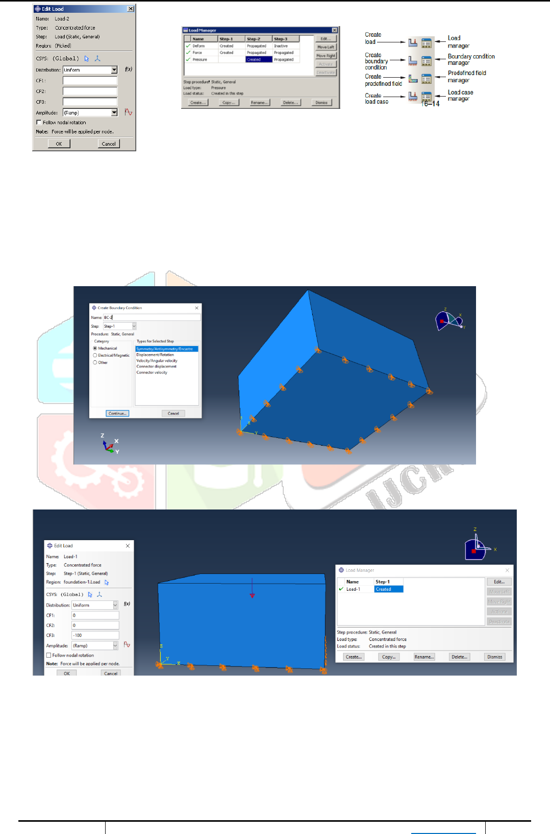
Figure 11 – Load toolbar and Load manager Module

 Boundary Conditions

is also an important module to check the specific point interaction. As Abaqus cannot apply real life constraints in model. So you

have to manually specify the predefined condition to be applied to a model to make analysis more effective and accurate (Pichler,

Pucker, Hamann, & Henke, High-Performance Abaqus simulations in soil mechanics reloaded - chances and frontiers, 2012).

Figure 12 – Fixed boundary condition at bottom

Figure 13 – Conc load applied with fixed boundary condition at bottom

IJCRT2110391

International Journal of Creative Research Thoughts (IJCRT) www.ijcrt.org

344

 Mesh

The Mesh module allows you to generate meshes on parts and assemblies created within Abaqus. Various levels of automation and

control are available so that you can create a mesh that meets the requirement of model for analysis. As with creating the parts and

assemblies, the process of assigning mesh attributes to the model—such as seeds, mesh techniques, and element types which is

feature based (Liu & Quek, 2014).

The Mesh module provides the following features:

• Tools for prescribing mesh density and global levels.

• Model colouring indicates the meshing technique is successful and assigned to each region in the model.

• A variety of mesh controls, such as:

– Element shape

– Meshing technique

– Meshing algorithm

– Adaptive remeshing rule

Seeds are markers that you place along the edges of a region to specify the target for mesh density in a region. Both the mesh density

along the boundary of the region and the mesh density in the interior of the region are determined by the seeds along the edges of the

region (Malik & Kumar, Effect of Blast Furnace Slag and Lime Mix on the Hydraulic Conductivity of Clay, 2016).

To create an acceptable mesh, you use the following process:

Assign mesh attributes and set mesh controls

The Mesh module provides different tools that allow you to specify different types of mesh characteristics, such as mesh density,

element shape, and element type.

Generate the mesh

The Mesh module uses a number of techniques to create meshes. The different mesh techniques provide you with different levels of

control.

Refine the mesh

The Mesh module provides a number of tools that allow you to refine the mesh:

– The seeding tools allow you to adjust the density of meshing.

– The Partition tool allows you to make a complex partition model to subregions.

– The Virtual Topology tool allows you to simplify your model by combining small faces/edges with adjacent faces and edges.

– The Edit Mesh toolset allows you to make minor adjustments to your mesh.

Optimize the mesh

You can assign remeshing rules to regions of your model.

Verify the mesh

The verification tools provide you with information regarding the quality of the elements which are used in the mesh.

IJCRT2110391

International Journal of Creative Research Thoughts (IJCRT) www.ijcrt.org

345

Figure 14 – Seeding part in Mesh

 Optimization

Is a process that generates results and analysis. You must combine the optimization results into a individual

output file to view the results of the optimization in the Visualization module (Dassault).

Figure 15 – Optimisation Chart (Dassault)

 Job

 In job module we create a job

 Check job from job manager by “Data Check”

 If no error is reported

 Submit the job

 Check results in Visualization Module

IJCRT2110391

International Journal of Creative Research Thoughts (IJCRT) www.ijcrt.org

346

 Visualization

Figure 16 – Visualizations of result

 Acknowledgment

The authors would like to acknowledge their respective institutions, Department of Civil Engineering, G. D. Goenka University

Gurugram Haryana INDIA. The dataset used for the experimentation has been obtained from the ABAQUS Software.

 Conflicts of Interest

The authors have no conflicts of interest to declare

IJCRT2110391

International Journal of Creative Research Thoughts (IJCRT) www.ijcrt.org

347

References

Abo-Elnor, M., Hamilton, R., & Boyle, J. T. (2003). Simulation of soil–blade interaction for sandy soil using advanced 3D finite element analysis.

Elsevier, 61-73.

Bathe, K. J. (2016). Finite element procedures. USA: Prentice Hall, Pearson Education, Inc.

Calvaranoa, L. S., Leonardia, G., & Palamaraa, R. (2017). Finite element modelling of unpaved road reinforced with geosynthetics. Elsevier, 99-

104.

Dassault. (n.d.). ABAQUS/CAE USER’S GUIDE. USA.

Dettmar, J. (2000). Finite elements projects. Clagary : University of calgary.

G. Hussein, M., & A. Meguid, M. (2013). Three-Dimensional Finite Element Analysis of Soil-Geogrid Interaction under Pull-out Loading

Condition. Geo Montreal.

Helwany, S. (2007). Applied Soil Mechanics with ABAQUS Applications.

Kanpur, I. (2021). An introduction to finite element software . kanpur, Uttar Pradesh.

Khennane, A. (2013). Introduction to finite element analysis using Abaqus. New York: Taylor & Francis Group.

Liu, G. R., & Quek, S. S. (2014). The finite element method. USA.

Malik, P., & Kumar, P. (2016). Effect of Blast Furnace Slag and Lime Mix on the Hydraulic Conductivity of Clay. IJIR, 1176-1179.

Malik, P., & Mishra, S. K. (2021). Geosynthetics Stabilizers and Fly Ash for Soil Subgrade Improvement – A State of the Art Review. International

Journal of Innovative Technology and Exploring Engineering, 97-104.

Malik, P., & Verma , N. (2015). Use of Geosynthetic Material To Improve the Properties of Subgrade Soil. International Journal of Engineering

Research & Technology, 298-300.

Mandal , J. N., & Ahirwar, S. K. (2017). Finite element analysis of flexible pavements with geogrids. elsevier, 411-416.

Pichler, T., Pucker, T., Hamann, T., & Henke, S. (2012). High-Performance Abaqus simulations in soil mechanics reloaded - chances and frontiers.

Research Gate .

Pichler, T., Pucker, T., Hamann, T., Henke, S., & Qiu, G. (2012). High Performance Abaqus simulations in soil mechanics reloaded chances.

SIMULIA Community Conference. SIMULIA Community Conference.

Stephansson, O., Jing, L., & Tsang, C. F. (1996). ABAQUS. Sweden: Elsevier Science.